Probing the Universe through the Stochastic Gravitational Wave Background

Abstract

Stochastic gravitational wave backgrounds, predicted in many models of the early universe and also generated by various astrophysical processes, are a powerful probe of the Universe. The spectral shape is key information to distinguish the origin of the background since different production mechanisms predict different shapes of the spectrum. In this paper, we investigate how precisely future gravitational wave detectors can determine the spectral shape using single and broken power-law templates. We consider the detector network of Advanced-LIGO, Advanced-Virgo and KAGRA and the space-based gravitational-wave detector DECIGO, and estimate the parameter space which could be explored by these detectors. We find that, when the spectrum changes its slope in the frequency range of the sensitivity, the broken power-law templates dramatically improve the $\chi^{2}$ fit compared with the single power-law templates and help to measure the shape with a good precision.

1 Introduction

Gravitational waves (GWs) would have been generated in the course of the evolution of the Universe from the very early era to the present. Since GWs can penetrate through space without attenuation, they carry invaluable information on phenomena in the very early Universe and astrophysical processes, which cannot be unraveled by other observations.

One such example is inflation, in which GWs as well as density perturbations are generated from quantum fluctuations [1, 2]. There are many other possible sources of GWs from the early Universe, such as first-order phase transition [4, 3, 5, 6, 7], preheating after inflation [8], topological defects [9, 10, 11, 12, 13], and so on. These GWs are considered as those from uncorrelated and unresolved sources and generate a stochastic background of GWs. Furthermore, various stochastic GW backgrounds of astrophysical origin have been discussed, such as binaries of compact objects (black holes, neutron stars, white dwarfs) [14, 15], stellar core collapse [16, 17], r-mode instability of neutron stars [18], magnetars [19] and so on. The detection of such stochastic GW backgrounds would give us an important insight on cosmology and astrophysics. In fact, the world-wide detector network of Advanced-LIGO (aLIGO), Advanced-Virgo (aVirgo) and KAGRA will increase the sensitivity of the GW background up to $\Omega_{\rm GW}\sim 10^{-9}$ at the frequency of $10-100$ Hz. In addition, the future space-based gravitational-wave detector Deci-Hertz Interferometer Gravitational-wave Observatory (DECIGO) [20, 21] might be able to detect stochastic GWs up to $\Omega_{\rm GW}\sim 10^{-16}$ at the frequency of $0.1-1$ Hz.

Since there are a lot of possible sources of stochastic GW backgrounds of various origins, we should prepare for its future detection. As described in Sec. 2, most of the spectra of stochastic GW backgrounds cannot be fitted by a single power-law as usually assumed but, rather, by a broken power-law, which can be characterized by two spectral indices, peak frequency, and amplitude. The spectral shape contains information on the source of the background, hence accurate modeling of the spectral shape would help to uncover the origin and the nature of this source. Fitting the stochastic background well-described by a broken power-law spectrum using a single power-law template would lead to a biased estimate of the spectral index, and useful information of the source would be lost. In this paper, focusing on the future detector network of aLIGO-aVirgo-KAGRA and the next-generation GW detectors such as DECIGO, we investigate how accurately we can extract the information on the parameters of the broken power-law templates from measurements of the spectrum of stochastic GW background (see [22], for an estimation of the number of templates required in the LIGO experiment in the stochastic GW background search with a broken power-law fit).

The organization of this paper is as follows. In Sec. 2, we review the sources of the stochastic GW background (cosmological ones in Sec. 2.1 and astrophysical ones in Sec. 2.2) and list the quantities characterizing the GW spectrum such as the amplitude, the spectral index and the frequency. In Sec. 3, we describe the method of the analysis to obtain expected constraints from future observations mainly by adopting the Fisher matrix and demonstrate how the parameter estimation is biased when we use an unsuitable template. In Sec. 4, we forecast the expected constraints on the parameters by the future detector network of aLIGO-aVirgo-KAGRA and the next-generation GW detector DECIGO. Sec. 5 is devoted to summary.

2 GW sources

In this section, we summarize (possible) GW sources of cosmological and astrophysical origins, which have been suggested in the literature. Here we do not intend to set a thorough list, but we discuss the sources which have been investigated relatively well.

GWs are described by the tensor perturbation $h_{ij}$ in the Friedmann-Robertson-Walker (FRW) spacetime:

$$ds^{2}=-dt^{2}+a^{2}(t)\left(\delta_{ij}+h_{ij}\right)dx^{i}dx^{j},$$ (2.1)

with $a(t)$ being the scale factor of the Universe. Here we consider a flat Universe and $h_{ij}$ satisfying the transverse-traceless condition: $\partial^{i}h_{ij}=h^{i}_{~{}i}=0$. The energy density of the GWs is given by

$$\rho_{\rm GW}=\frac{1}{64\pi G}\left\langle(\partial_{t}h_{ij})^{2}+\left(\frac{\nabla}{a}h_{ij}\right)^{2}\right\rangle,$$ (2.2)

where the bracket describes the spatial average.

To characterize the spectral amplitude of GWs, we use the dimensionless quantity $\Omega_{\rm GW}$, which describes the energy density of GWs per logarithmic interval of the frequency $f$ at the present time, normalized by the critical density $\rho_{\rm crit}=3H_{0}^{2}/(8\pi G)$:

$$\Omega_{\rm GW}\equiv\frac{1}{\rho_{\rm crit}}\frac{d\rho_{\rm GW}}{d\ln f}.$$ (2.3)

One may approximate the GW spectrum using a broken power-law as

$$\Omega_{\rm GW}(f)=\begin{cases}&\Omega_{\rm GW\ast}\left(\displaystyle\frac{f}{f_{\ast}}\right)^{n_{\rm GW1}}\qquad\text{for}~{}~{}f<f_{\ast},\\ \\ &\Omega_{\rm GW\ast}\left(\displaystyle\frac{f}{f_{\ast}}\right)^{n_{\rm GW2}}~{}~{}\qquad\text{for}~{}~{}f>f_{\ast},\end{cases}$$ (2.4)

where $\Omega_{\rm GW*}$ is the amplitude at $f=f_{\ast}$ (the peak frequency or the reference frequency) with $f_{\ast}$ being the frequency at which the spectral dependence changes, and $n_{\rm GW1}$ and $n_{\rm GW2}$ are the spectral index for $f<f_{\ast}$ and $f>f_{\ast}$, respectively. Although not all the models can well be described by this simple form, in the following, we provide typical values of $\Omega_{\ast},f_{\ast},n_{\rm GW1}$ and $n_{\rm GW2}$ for various cosmological and astrophysical stochastic backgrounds.

2.1 Cosmological sources

First, we list cosmological sources. See also [23, 24] for a collection of some cosmological sources. All the models we describe in this subsection are summarized in Table LABEL:table:cosmological.

$\bullet$ First-order phase transition
It has been argued that significant GWs can be generated during first-order phase transition in the early universe (for example, an electroweak-scale phase transition [25, 26]). The GW spectrum depends on the mechanisms taking place during the phase transition. There are three processes generating GWs: bubble collision, turbulence and sound waves. Below, we quote the spectral indices, the peak frequency and the amplitude of the GW spectrum from these processes separately .

(i) Bubble collision [4, 5, 29, 30, 31]
In a first-order phase transition, bubbles are nucleated. They rapidly expand and collide, sourcing a large amount of GWs. The GWs from bubble collision has spectral indices

$$n_{\rm GW1}=2.8,\qquad n_{\rm GW2}=-1,$$ (2.5)

The peak frequency of the GWs generated at the time of phase transition is written as

$$f_{\rm PT}=\beta\left(\displaystyle\frac{0.62}{1.8-0.1v_{w}+v_{w}^{2}}\right),$$ (2.6)

with $v_{w}$ being the bubble wall velocity. When it is redshifted to the present-day frequency, we have

$$f_{\ast}\sim 10^{-5}\left(\displaystyle\frac{f_{\rm PT}}{\beta}\right)\left(\displaystyle\frac{\beta}{H_{\rm PT}}\right)\left(\displaystyle\frac{T_{\rm PT}}{100~{}{\rm GeV}}\right)\quad{\rm[Hz]},$$ (2.7)

where $\beta\simeq\dot{\Gamma}/\Gamma$ with $\Gamma$ being the bubble nucleation rate, and $H_{\rm PT}$ and $T_{\rm PT}$ are the Hubble rate and the temperature at the time of the phase transition. The amplitude at peak frequency today is given by

$$\Omega_{\rm GW\ast}\sim 10^{-5}\left(\displaystyle\frac{H_{\rm PT}}{\beta}\right)^{2}\left(\displaystyle\frac{\kappa_{\phi}\alpha}{1+\alpha}\right)^{2}\left(\displaystyle\frac{0.11v_{w}^{3}}{0.42+v_{w}^{2}}\right),$$ (2.8)

where $\kappa_{\phi}$ is the fraction of the vacuum energy converted into the gradient energy of a scalar field. For analytic calculations, see [29, 32, 33, 34].

(ii) Turbulence [6, 23, 35, 31]
Subsequent magnetohydrodynamic (MHD) turbulent cascades after bubble collisions also source GWs. The spectral indices, the peak frequency and the present-day amplitude can be written as

$$n_{\rm GW1}=3,\qquad n_{\rm GW2}=-\frac{5}{3},$$ (2.9)

$$f_{\ast}\sim 3\times 10^{-5}\left(\displaystyle\frac{1}{v_{w}}\right)\left(\displaystyle\frac{\beta}{H_{\rm PT}}\right)\left(\displaystyle\frac{T_{\rm PT}}{100~{}{\rm GeV}}\right)\quad{\rm[Hz]},$$ (2.10)

$$\Omega_{\rm GW\ast}\sim 3\times 10^{-4}\left(\displaystyle\frac{H_{\rm PT}}{\beta}\right)\left(\displaystyle\frac{\kappa_{\rm turb}\alpha}{1+\alpha}\right)^{3/2}v_{w},$$ (2.11)

where $\kappa_{\rm turb}$ is the fraction of latent heat converted into turbulence.

(iii) Sound waves [7, 31, 36]
Sound waves in the plasma fluid are also an important source of GWs. For the case of sound waves, $n_{\rm GW1},n_{\rm GW2},f_{\ast}$ and $\Omega_{\rm GW\ast}$ are given by

$$n_{\rm GW1}=3,\qquad n_{\rm GW2}=-4,$$ (2.12)

$$f_{\ast}\sim 2\times 10^{-5}\left(\displaystyle\frac{1}{v_{w}}\right)\left(\displaystyle\frac{\beta}{H_{\rm PT}}\right)\left(\displaystyle\frac{T}{100~{}{\rm GeV}}\right)\quad{\rm[Hz]},$$ (2.13)

$$\Omega_{\rm GW\ast}\sim 3\times 10^{-6}\left(\displaystyle\frac{H_{\rm PT}}{\beta}\right)\left(\displaystyle\frac{\kappa_{v}\alpha}{1+\alpha}\right)^{2}v_{w},$$ (2.14)

where $\kappa_{v}$ is the fraction of latent heat converted into the bulk motion of the fluid. For a recent study of GWs from sound waves, see [37].

$\bullet$ Preheating
During preheating stage, GWs can be generated from violent production of particles via a parametric resonance (see [38, 39] for a recent review on preheating), and there have been a lot of studies on the generation of GWs from preheating (see [8] for a pioneering work). Although a numerical simulation is needed to precisely calculate the GW spectrum, here we describe some approximate (fitting) formula for the GW spectrum. Below, we present only the cases of preheating into scalars, but preheating into gauge fields is also studied in the literature [40, 41, 42].

(i) Case with $V=\displaystyle\frac{1}{4}\lambda\phi^{4}$
First, let us consider a model with

$$V(\phi,\chi)=\displaystyle\frac{1}{4}\lambda\phi^{4}+\frac{1}{2}g\phi^{2}\chi^{2},$$ (2.15)

where $\phi$ is the inflaton which decays into another scalar field $\chi$. Although a quartic chaotic inflation model is now ruled out by Planck data, for reference, we fix the value of $\lambda$ to give the right amplitude of primordial density fluctuations, i.e., $\lambda\simeq 10^{-14}$. In this model, the spectral indices are given by

$$n_{\rm GW1}=3,\qquad n_{\rm GW2}={\rm cutoff}.$$ (2.16)

At higher frequency, the GW spectrum decays exponentially and cannot be well fitted by a constant power law. From now on, we denote such a case as “cutoff”. Once we fix the value of $\lambda$, i.e, the inflation scale, the peak frequency is approximately fixed as [43]

$$f_{\ast}\sim 10^{7}\quad{\rm[Hz]}.$$ (2.17)

Ref. [43] has shown that the peak amplitude can be fitted to the so-called resonance parameter $q(=g^{2}/\lambda)$. Since the amplitude oscillates depending on $q$, we give a range in the formula below:

$$3.4\times 10^{-12}\left(\frac{q}{100}\right)^{-0.42}<\Omega_{\rm GW\ast}h^{2}<2.4\times 10^{-11}\left(\frac{q}{100}\right)^{-0.56},$$ (2.18)

where $h$ is the reduced Hubble constant. Thus, roughly speaking, the peak amplitude is

$$\Omega_{\rm GW\ast}\sim 10^{-11}\left(\frac{q}{100}\right)^{-0.5}.$$ (2.19)

(ii) Hybrid [44, 45]
For a hybrid-type inflationary model, the potential can be given by

$$V=\frac{1}{4}\lambda\left(\sigma^{2}-v^{2}\right)^{2}+\frac{1}{2}g^{2}\phi^{2}\sigma^{2}+V_{\rm inf}(\phi),$$ (2.20)

where $\phi$ is the inflaton, $V_{\rm inf}(\phi)$ is its potential controlling the inflationary dynamics during inflation, $\lambda$ and $g$ are coupling constants, and $v$ is the VEV of a field $\sigma$. But we do not need to specify it here since the generation of GWs from preheating does not depend on the details of the potential during inflation. For this model, the spectral indices, the peak frequency and the amplitudes can be roughly given as, for the case of $g^{2}/\lambda\ll 1$,

$$n_{\rm GW1}=2,\qquad n_{\rm GW2}={\rm cutoff},$$ (2.21)

$$f_{\ast}\sim\frac{g}{\sqrt{\lambda}}\lambda^{1/4}10^{10.25}\quad{\rm[Hz]},$$ (2.22)

$$\Omega_{\rm GW\ast}\sim 10^{-5}\left(\frac{\lambda}{g^{2}}\right)^{1.16}\left(\frac{v}{M_{\rm pl}}\right)^{2}.$$ (2.23)

$\bullet$ Cosmic strings [9, 10]
Cosmic strings are one-dimensional topological defects, which arise naturally in field theories, as well as in inflationary scenarios based on superstring theory. They are known to emit strong GW bursts from pathological structures, such as cusps and kinks [11], during their evolution. When GWs from all the strings are numerous, their signals overlap and become a stochastic GW background.

(i) Loops 1 [46, 47, 48, 49, 50, 51, 52, 53, 54, 23, 55, 56, 57]
Cosmic string loops are known to generate a GW background at high frequencies. The loops formed in the late matter-dominated era give rise to a GW background with a peak-like shape. Taking into account the uncertainties in the string network modeling, the spectral indices roughly range as

$$n_{\rm GW1}=[1,2],\qquad n_{\rm GW2}=[-1,-0.1],$$ (2.24)

with

$$f_{\ast}\sim 3\times 10^{-8}\left(\frac{G\mu}{10^{-11}}\right)^{-1}\quad{\rm[Hz]},$$ (2.25)

where $G$ is the gravitational constant and $\mu$ is the string tension. Note that this dependence holds only for $\alpha_{\rm loop}\gg\Gamma G\mu$ where $\Gamma$ characterizes GW emission efficiency and $\alpha_{\rm loop}$ is the typical initial size of loops normalized with respect to the loop formation time $t_{i}$. When $\alpha_{\rm loop}\gg\Gamma G\mu$, the dependence is

$$f_{\ast}\sim 3\times 10^{-8}\left(\frac{\alpha_{\rm loop}}{10^{-9}}\right)^{-1}\quad{\rm[Hz]},$$ (2.26)

The amplitude strongly depends on the string parameters such as tension $G\mu$ and initial loop size $\alpha_{\rm loop}$. When one considers $\alpha_{\rm loop}\gg\Gamma G\mu$, the amplitude at peak is roughly given by

$$\Omega_{\rm GW\ast}\sim 10^{-9}\left(\frac{G\mu}{10^{-12}}\right)\left(\frac{\alpha_{\rm loop}}{10^{-1}}\right)^{-1/2}.$$ (2.27)

For $\alpha_{\rm loop}\ll\Gamma G\mu$, the parameter dependence becomes

$$\Omega_{\rm GW\ast}\sim 10^{-12}\left(\frac{G\mu}{10^{-12}}\right).$$ (2.28)

Note that, in the case of cosmic superstrings, the reconnection probability also affects the amplitude.

(ii) Loops 2 [46, 47, 48, 49, 50, 51, 52, 53, 54, 23, 55, 56, 57]
At higher frequencies, GWs from loops formed during the radiation-dominated era are the dominant contribution and the spectrum becomes flat. Thus, around the intermediate frequency where we see both contributions from loops formed in the radiation-dominated and the matter-dominated phases, the spectral indices change as

$$n_{\rm GW1}=[-1,-0.1],\qquad n_{\rm GW2}=0.$$ (2.29)

The transition frequency and the amplitude strongly depends on the modeling of the cosmic string network and the calculation method, but the rough expectation is

$$f_{\ast}\sim 3\times 10^{-5}\left(\displaystyle\frac{G\mu}{10^{-11}}\right)^{-1}\quad{\rm[Hz]},$$ (2.30)

$$\Omega_{\rm GW\ast}\sim 10^{-9.5}\left(\frac{G\mu}{10^{-12}}\right)\left(\frac{\alpha_{\rm loop}}{10^{-1}}\right)^{-1/2},$$ (2.31)

for $\alpha_{\rm loop}\gg\Gamma G\mu$, and

$$f_{\ast}\sim 3\times 10^{-3}\left(\displaystyle\frac{\alpha_{\rm loop}}{10^{-9}}\right)^{-1}\quad{\rm[Hz]},$$ (2.32)

$$\Omega_{\rm GW\ast}\sim 10^{-14}\left(\frac{G\mu}{10^{-12}}\right),$$ (2.33)

for $\alpha_{\rm loop}\ll\Gamma G\mu$.

(iii) Infinite strings [58, 59]
Kinks on infinite strings generate a GW background over all frequencies. Typically, the amplitude is smaller than the one from loops, but it becomes important at low frequencies where loops do not emit GWs. The spectral index slightly depends on the expansion rate of the Universe when kinks are generated, but typically the spectrum is almost flat. When combined with the GWs from loops which produce GWs at high frequencies, one may find a break in the spectrum such as

$$n_{\rm GW1}=[0,0.2],\qquad n_{\rm GW2}=[1,2],$$ (2.34)

The transition frequency is highly model dependent since parameter dependencies of GW spectra from loops and infinite strings are different, and hence we do not set a value for $f_{\ast}$. For a typical parameter choice, the GW amplitude can be roughly given by

$$\Omega_{\rm GW\ast}\sim 10^{-12}\left(\frac{G\mu}{10^{-8}}\right).$$ (2.35)

The prefactor can vary depending on the transition frequency, but it should be in the range of $[10^{-11},10^{-13}]$ for $G\mu=10^{-8}$.

$\bullet$ Domain walls [9, 60, 61, 62, 63]
The existence of domain walls is in conflict with cosmological observations, since their energy density easily dominates that of the universe. However, this problem can be avoided by considering unstable domain walls and their annihilation in the early Universe may produce a significant amount of gravitational waves.

Numerical simulations [61, 62, 63] find the spectral dependencies of the power spectrum as

$$n_{\rm GW1}=3,\qquad n_{\rm GW2}=-1,$$ (2.36)

with typical frequency

$$f_{\ast}\sim 10^{-9}\left(\displaystyle\frac{T_{\rm ann}}{10^{-2}{\rm GeV}}\right)\quad{\rm[Hz]},$$ (2.37)

where $T_{\rm ann}$ is the temperature of the universe at domain wall annihilation. The amplitude is determined by the domain wall tension $\sigma$ as

$$\Omega_{\rm GW\ast}\sim 10^{-17}\left(\displaystyle\frac{\sigma}{1{\rm TeV}^{3}}\right)^{2}\left(\displaystyle\frac{T_{\rm ann}}{10^{-2}{\rm GeV}}\right)^{-4}.$$ (2.38)

$\bullet$ Self-ordering scalar fields [12]
A phase transition which breaks global O($N$) symmetry of scalar fields generates a spatial gradient of the scalar fields on superhorizon scales, because each causally disconnected region of the Universe gets arbitrarily different directions of the fields. When the modes re-enter the horizon, the fields release gradient energy by the self-ordering of the Nambu-Goldstone modes, and they continuously source GWs at the horizon scale.

(i) Radiation-dominated phase [64, 13, 65, 66]
If all the GW modes of interest enter the horizon during the radiation-dominated phase, GWs have a scale-invariant spectrum at the frequencies of interferometer experiments, and hence we have

$$n_{\rm GW1}=0,\qquad n_{\rm GW2}=0.$$ (2.39)

Therefore, there is no well-defined peak frequency $f_{\ast}$ in this model. The spectral amplitude depends on the number of the scalar field components $N$ and the VEV of the fields $v$,

$$\Omega_{\rm GW\ast}\sim\displaystyle\frac{511}{N}\Omega_{\rm rad}\left(\displaystyle\frac{v}{M_{\rm pl}}\right)^{4}.$$ (2.40)

(ii) Effect of reheating [67]
The frequency dependence of the GW spectrum is affected by the expansion rate of the Universe. If the expansion rate of the Universe evolves like a matter-dominated phase during reheating, the spectral indices are

$$n_{\rm GW1}=0,\qquad n_{\rm GW2}=-2,$$ (2.41)

and the peak frequency can be written as

$$f_{\ast}\sim 0.4\left(\displaystyle\frac{T_{R}}{10^{7}~{}{\rm GeV}}\right)\quad{\rm[Hz]},$$ (2.42)

where $T_{R}$ is the temperature of the Universe when reheating is completed. The flat part $n_{\rm GW1}=0$ corresponds to the modes which enter the horizon during the radiation-dominated phase after reheating, and its amplitude is given as in Eq. (2.40), while the amplitude of the modes which enter during reheating is suppressed. So the amplitude is

$$\Omega_{\rm GW\ast}\sim\displaystyle\frac{511}{N}\Omega_{\rm rad}\left(\displaystyle\frac{v}{M_{\rm pl}}\right)^{4}.$$ (2.43)

$\bullet$ Magnetic field [68, 69]
Magnetic fields are considered to be present at almost all scales in the Universe. In particular, they exist even in the intergalactic medium [70], which may have originated in the early Universe. It has been argued that such primordial magnetic fields can arise from inflation [71, 72], phase transition [73, 74] and so on. Here we describe the GW power spectrum having magnetic fields generated from phase transition in mind. The slope of the power spectrum is predicted to be

$$n_{\rm GW1}=3,\qquad n_{\rm GW2}=\alpha_{B}+1,$$ (2.44)

where we have assumed that the initial magnetic field power spectrum is given by $P_{B}\propto k^{2}$ and $\propto k^{\alpha_{B}}$ for scales larger and smaller than the correlation scale respectively [69], and the correlation length and the horizon scale at the generation time are identical. The characteristic frequency and the amplitude at which the slope of the GW spectrum changes can be roughly estimated as

$$f_{\ast}\sim 10^{-6}\left(\frac{T_{\ast}}{100~{}{\rm GeV}}\right)\quad{\rm[Hz]},$$ (2.45)

$$\Omega_{\rm GW\ast}\sim 10^{-16}\left(\frac{B}{10^{-10}~{}{\rm G}}\right),$$ (2.46)

where $T_{\ast}$ corresponds to the temperature at the production of magnetic fields and $B$ is the magnetic field magnitude today.

$\bullet$ Inflation+reheating [75]
Inflation generates almost scale-invariant GWs originating from the quantum fluctuations in spacetime. The primordial tensor power spectrum is given by

$${\cal P}_{\rm inf}=\frac{8}{M_{\rm pl}^{2}}\left(\frac{H_{\ast}}{2\pi}\right)^{2},$$ (2.47)

where $H_{\ast}$ is the Hubble parameter at the horizon exit during inflation and it is almost constant in the standard slow-roll inflationary models. The present-day GW spectrum can be given by using the transfer function $T(k)$, which describes the evolution of GWs after inflation,

$$\Omega_{\rm GW}(k)=\frac{1}{12}\left(\frac{k}{aH}\right)^{2}T^{2}(k){\cal P}_{\rm inf}(k),$$ (2.48)

where $k=2\pi f$ is the wavenumber. The explicit form of $T(k)$ is given in [76, 77, 78, 79].

In the standard scenario, the inflaton oscillates at the bottom of its potential during reheating. In such phase, the Universe behaves as matter-dominated one if the inflaton potential has a quadratic form at its bottom. For modes entering the horizon during the matter-dominated epoch, the transfer function scales as $T(k)\propto k^{-2}$. On the other hand, the modes entering the horizon during the radiation-dominated epoch is $T(k)\propto k^{-1}$. Because of the transition from the matter-dominated epoch to the radiation-dominated one at the end of reheating, the spectrum has

$$n_{\rm GW1}\sim 0,\qquad n_{\rm GW2}=-2.$$ (2.49)

More precisely, $n_{\rm GW1}$ can be given by $n_{\rm GW1}=-2\epsilon$ with $\epsilon=-\dot{H}/H^{2}$ being the first slow-roll parameter, where, however, $|n_{\rm GW1}|\ll{\cal O}(1)$ in general.

The characteristic frequency $f_{\ast}$ corresponds to the mode which enters the horizon at the time of reheating. Therefore, it can be given as a function of the reheating temperature as

$$f_{\ast}\sim 0.3\left(\displaystyle\frac{T_{R}}{10^{7}~{}{\rm GeV}}\right)\quad{\rm[Hz]}.$$ (2.50)

By using the tensor-to-scalar ratio, the amplitude $\Omega_{\rm GW\ast}$ is given by

$$\Omega_{\rm GW\ast}\sim 2\times 10^{-17}\left(\displaystyle\frac{r}{0.01}\right).$$ (2.51)

$\bullet$ Inflation+kination [81, 80, 82, 83, 84, 85]
In some scenarios of the early Universe, the radiation-dominated epoch is preceded by the so-called kination epoch, in which the energy density of the Universe is dominated by the kinetic energy of a scalar field. Examples of this type of model include quintessential inflation [81]. During the kination epoch, the Hubble expansion rate decreases as $H\propto a^{-3}$ (the energy density of the scalar field scales as $\rho_{\phi}\propto a^{-6}$, which gives the transfer function of $T(k)\propto k^{2}$. Therefore, the spectral indices for the GW spectrum are given by

$$n_{\rm GW1}\sim 0,\qquad n_{\rm GW2}=1.$$ (2.52)

We note that here again $n_{\rm GW1}$ is given by $n_{\rm GW1}=-2\epsilon$ which is close to 0. The characteristic frequency corresponds to the mode entering the horizon at the end of the kination epoch. By denoting the temperature at this epoch by $T_{\rm kin}$, $f_{\ast}$ is given by

$$f_{\ast}\sim 0.3\left(\displaystyle\frac{T_{\rm kin}}{10^{7}~{}{\rm GeV}}\right)\quad{\rm[Hz]}.$$ (2.53)

The amplitude is given in the same way as for the inflation+reheating case:

$$\Omega_{\rm GW\ast}\sim 2\times 10^{-17}\left(\displaystyle\frac{r}{0.01}\right).$$ (2.54)

$\bullet$ Particle production during inflation [87, 86, 88]
It has been argued that large GWs can be produced from particle production during inflation [87, 86, 88]. Let us consider a model where the inflaton $\phi$ couples to a $U(1)$ gauge field $F_{\mu\nu}$ as

$${\cal L}\supset-\frac{\phi}{4f}F_{\mu\nu}\tilde{F}^{\mu\nu},$$ (2.55)

with $f$ being a coupling constant with the dimension of mass. In this model, gauge quanta can be significantly produced, which sources the GWs. The primordial GW power spectrum is given by the sum of the contributions from the usual inflationary vacuum and the particle production ones, which can be written as [95, 96]

$$P_{\rm GW}(k)=\frac{2H_{\ast}^{2}}{\pi^{2}M_{\rm pl}^{2}}+8.7\times 10^{-8}\frac{H_{\ast}^{4}}{M_{\rm pl}^{4}}\frac{e^{4\pi\xi}}{\xi^{6}},$$ (2.56)

where $\xi$ is defined by

$$\xi\equiv\frac{d\phi/dt}{2fH_{\ast}}.$$ (2.57)

On large scale (low frequency), the contribution from the usual inflationary vacuum dominates, while on small scales (high frequency), the one from the particle production does. Therefore the spectral indices are written as [88]

$$n_{\rm GW1}=-2\epsilon\sim 0,\qquad n_{\rm GW2}=-4\epsilon+(4\pi\xi-6)(\epsilon-\eta).$$ (2.58)

The transition frequency corresponds to the one at which the GW spectrum from particle production gets dominated over the one from the usual inflationary tensor mode. The GW production from particle production is sensitive to the parameters in the model such as $\xi$, and thus the transition frequency is highly dependent on the model parameters (see e.g., [97]).

The amplitude at the transition frequency is given as the same as the one from the usual inflationary vacuum (assuming an almost scale-invariant GW spectrum on lower frequency region), and hence it can be written as

$$\Omega_{\rm GW\ast}\sim 2\times 10^{-17}\left(\displaystyle\frac{r}{0.01}\right).$$ (2.59)

$\bullet$ 2nd-order perturbations
At 2nd order in the cosmological perturbation theory, the scalar, vector and tensor modes cannot be separated and they could affect one another. Typically the amplitude of the GWs generated from 2nd-order scalar perturbations in standard slow-roll inflation is very small when one considers the radiation-dominated epoch after inflation [98]. However, considering a different Hubble expansion of the Universe [99] or non-scale-invariant scalar perturbations, we can expect a large GW amplitude. For the latter, we introduce only the case related to primordial black hole (PBH) formation [100], but the existence of other fields such as curvaton [101] and instability of the standard model Higgs [102] can also induce GWs with large amplitude.

(i) Early matter phase [99]
In [99, 103], it has been argued that 2nd-order scalar perturbations induce the tensor mode which might be detectable in the future GW observations if the Universe went through an early matter-dominated phase. When we consider the scale invariant spectrum of scalar perturbations, the spectral indices of GWs are given by

$$n_{\rm GW1}=1,\qquad n_{\rm GW2}=\textrm{drop-off}.$$ (2.60)

The spectrum drops off sharply at the scale corresponding to the end of inflation. Therefore here we denote $n_{\rm GW2}$ as “drop-off”. Note that these indices change depending on the spectral shape of the primordial scalar perturbations [104]. The typical frequency is given by the reheating temperature $T_{\rm reh}$ and the energy scale of inflation $M_{\rm inf}$,

$$f_{\ast}\sim 7\times 10^{5}\left(\displaystyle\frac{T_{\rm reh}}{10^{9}~{}{\rm GeV}}\right)^{1/3}\left(\displaystyle\frac{M_{\rm inf}}{10^{16}~{}{\rm GeV}}\right)^{2/3}\quad{\rm[Hz]},$$ (2.61)

and the amplitude is given by

$$\Omega_{\rm GW\ast}\sim 10^{-12}\left(\displaystyle\frac{T_{\rm reh}}{10^{9}~{}{\rm GeV}}\right)^{-4/3}\left(\displaystyle\frac{M_{\rm inf}}{10^{16}~{}{\rm GeV}}\right)^{4/3}.$$ (2.62)

(ii) Primordial black holes [100]
PBHs can form when density fluctuations with large amplitude are generated by some mechanism and such large scalar fluctuations induce GWs as a second-order effect as discussed above. If we assume primordial scalar fluctuations with a peak-like shape, we can approximate the power spectrum as a delta function as follows:

$${\cal P}_{\zeta}(k)={\cal A}^{2}\delta(\ln(k/k_{p})),$$ (2.63)

where ${\cal A}^{2}$ and $k_{p}$ are the amplitude and the wavenumber at the peak. With this kind of sharp scalar fluctuations, we also expect GW generation and the spectrum is

$$n_{\rm GW1}=2,\qquad n_{\rm GW2}=\textrm{drop-off},$$ (2.64)

The spectrum drops off at the scale corresponding to the peak of scalar fluctuations, which is related to the mass of the PBH $M_{\rm PBH}$ as

$$f_{\ast}\sim 4\times 10^{-2}\left(\frac{M_{\rm PBH}}{10^{20}~{}{\rm g}}\right)^{-1/2}\quad{\rm[Hz]}.$$ (2.65)

The amplitude at the peak is

$$\Omega_{\rm GW\ast}\sim 7\times 10^{-9}\left(\frac{{\cal A}^{2}}{10^{-3}}\right)^{2}.$$ (2.66)

Note that the shape of the GW spectrum is different in the cases where the power spectrum of fluctuation is amplified in a broad range of scales and cannot be approximated by a delta function [105].

$\bullet$ Pre-Big-Bang [106, 107, 109, 110]
In a string theory-inspired cosmological scenario, the so-called pre-big bang model, a blue-tilted GW spectrum can be generated. In particular, the lower frequency part of the spectrum is blue-tilted, while on higher frequency, it can be flat or red/blue-tilted (see [108] for a recent update and the detailed spectrum). The spectral index for lower and higher frequency parts is given by [106]

$$n_{\rm GW1}=3,\qquad n_{\rm GW2}=3-2\mu,$$ (2.67)

where $\mu$ describes the growth of the dilaton during stringy phase and $\mu\geq 0$. The transition frequency corresponds to the one at which the mode crosses the horizon at the beginning of the string phase, which can be regarded as a model parameter in this scenario and there is no typical phase. However, it has been argued that this frequency can be around the one where LISA or aLIGO are sensitive. The amplitude of the GW spectrum is estimated as

$$\Omega_{\rm GW\ast}\sim 1.4\times 10^{-6}\left(\frac{H_{s}}{0.15M_{\rm pl}}\right)^{4},$$ (2.68)

where $H_{s}$ is the Hubble parameter during the stringy phase.

Table 1: Cosmological GW sources

source	$n_{\rm GW1}$	$n_{\rm GW2}$	$f_{\ast}$ [Hz]	$\Omega_{\rm GW}$
Phase transition (bubble collision)	$2.8$	$-2$	$\sim 10^{-5}\left(\displaystyle\frac{f_{\rm PT}}{\beta}\right)\left(\displaystyle\frac{\beta}{H_{\rm PT}}\right)\left(\displaystyle\frac{T_{\rm PT}}{100~{}{\rm GeV}}\right)$	$\sim 10^{-5}\left(\displaystyle\frac{H_{\rm PT}}{\beta}\right)^{2}\left(\displaystyle\frac{\kappa_{\phi}\alpha}{1+\alpha}\right)^{2}\left(\displaystyle\frac{0.11v_{w}^{3}}{0.42+v_{w}^{2}}\right)$
Phase transition (turbulence)	$3$	$-5/3$	$\sim 3\times 10^{-5}\left(\displaystyle\frac{1}{v_{w}}\right)\left(\displaystyle\frac{\beta}{H_{\rm PT}}\right)\left(\displaystyle\frac{T_{\rm PT}}{100~{}{\rm GeV}}\right)$	$\sim 3\times 10^{-4}\left(\displaystyle\frac{H_{\rm PT}}{\beta}\right)\left(\displaystyle\frac{\kappa_{\rm turb}\alpha}{1+\alpha}\right)^{3/2}v_{w}$
Phase transition (sound waves)	$3$	$-4$	$\sim 2\times 10^{-5}\left(\displaystyle\frac{1}{v_{w}}\right)\left(\displaystyle\frac{\beta}{H_{\rm PT}}\right)\left(\displaystyle\frac{T_{\rm PT}}{100~{}{\rm GeV}}\right)$	$\sim 3\times 10^{-6}\left(\displaystyle\frac{H_{\rm PT}}{\beta}\right)\left(\displaystyle\frac{\kappa_{v}\alpha}{1+\alpha}\right)^{2}v_{w}$
Preheating ($\lambda\phi^{4}$)	$3$	cutoff	$\sim 10^{7}$	$\sim 10^{-11}\left(\displaystyle\frac{g^{2}/\lambda}{100}\right)^{-0.5}$
Preheating (hybrid)	$2$	cutoff	$\sim\displaystyle\frac{g}{\sqrt{\lambda}}\lambda^{1/4}10^{10.25}$	$\sim 10^{-5}\left(\displaystyle\frac{\lambda}{g^{2}}\right)^{1.16}\left(\displaystyle\frac{v}{M_{\rm pl}}\right)^{2}$
Cosmic strings (loops 1)	$[1,2]$	$[-1,-0.1]$	$\sim 3\times 10^{-8}\left(\displaystyle\frac{G\mu}{10^{-11}}\right)^{-1}$	$\sim 10^{-9}\left(\displaystyle\frac{G\mu}{10^{-12}}\right)\left(\displaystyle\frac{\alpha_{\rm loop}}{10^{-1}}\right)^{-1/2}$ (for $\alpha_{\rm loop}\gg\Gamma G\mu$)
Cosmic strings (loops 2)	$[-1,-0.1]$	$0$	$\sim 3\times 10^{-8}\left(\displaystyle\frac{G\mu}{10^{-11}}\right)^{-1}$	$\sim 10^{-9.5}\left(\displaystyle\frac{G\mu}{10^{-12}}\right)\left(\displaystyle\frac{\alpha_{\rm loop}}{10^{-1}}\right)^{-1/2}$ (for $\alpha_{\rm loop}\gg\Gamma G\mu$)
Cosmic strings (infinite strings)	$[0,0.2]$	$[0,0.2]$	—	$\sim 10^{-[11,13]}\left(\frac{G\mu}{10^{-8}}\right)$
Domain walls	3	-1	$\sim 10^{-9}\left(\displaystyle\frac{T_{\rm ann}}{10^{-2}{\rm GeV}}\right)$	$\sim 10^{-17}\left(\displaystyle\frac{\sigma}{1{\rm TeV}^{3}}\right)^{2}\left(\displaystyle\frac{T_{\rm ann}}{10^{-2}{\rm GeV}}\right)^{-4}$
Self-ordering scalar fields	$0$	$0$	—	$\sim\displaystyle\frac{511}{N}\Omega_{\rm rad}\left(\displaystyle\frac{v}{M_{\rm pl}}\right)^{4}$
Self-ordering scalar + reheating	$0$	$-2$	$\sim 0.4\left(\displaystyle\frac{T_{R}}{10^{7}~{}{\rm GeV}}\right)$	$\sim\displaystyle\frac{511}{N}\Omega_{\rm rad}\left(\displaystyle\frac{v}{M_{\rm pl}}\right)^{4}$
Magnetic fields	$3$	$\alpha_{B}+1$	$\sim 10^{-6}\left(\displaystyle\frac{T_{\ast}}{10^{2}{\rm GeV}}\right)$	$\sim 10^{-16}\left(\displaystyle\frac{B}{10^{-10}{\rm G}}\right)$
Inflation+reheating	$\sim 0$	$-2$	$\sim 0.3\left(\displaystyle\frac{T_{R}}{10^{7}~{}{\rm GeV}}\right)$	$\sim 2\times 10^{-17}\left(\displaystyle\frac{r}{0.01}\right)$
Inflation+kination	$\sim 0$	1	$\sim 0.3\left(\displaystyle\frac{T_{R}}{10^{7}~{}{\rm GeV}}\right)$	$\sim 2\times 10^{-17}\left(\displaystyle\frac{r}{0.01}\right)$
Particle prod. during inf.	$-2\epsilon$	$-4\epsilon(4\pi\xi-6)(\epsilon-\eta)$	—	$\sim 2\times 10^{-17}\left(\displaystyle\frac{r}{0.01}\right)$
2nd-order (inflation)	$1$	drop-off	$\sim 7\times 10^{5}\left(\displaystyle\frac{T_{\rm reh}}{10^{9}~{}{\rm GeV}}\right)^{1/3}\left(\displaystyle\frac{M_{\rm inf}}{10^{16}~{}{\rm GeV}}\right)^{2/3}$	$\sim 10^{-12}\left(\displaystyle\frac{T_{\rm reh}}{10^{9}~{}{\rm GeV}}\right)^{-4/3}\left(\displaystyle\frac{M_{\rm inf}}{10^{16}~{}{\rm GeV}}\right)^{4/3}$
2nd-order (PBHs)	$2$	drop-off	$\sim 4\times 10^{-2}\left(\displaystyle\frac{M_{\rm PBH}}{10^{20}~{}{\rm g}}\right)^{-1/2}$	$\sim 7\times 10^{-9}\left(\displaystyle\frac{{\cal A}^{2}}{10^{-3}}\right)^{2}$
Pre-Big-Bang	$3$	$3-2\mu$	—	$\sim 1.4\times 10^{-6}\left(\displaystyle\frac{H_{s}}{0.15M_{\rm pl}}\right)^{4}$

2.2 Astrophysical sources

Here, we list astrophysical sources. See also [111] for a collection of some astrophysical sources. All the models we describe in this subsection are summarized in Table 2.

$\bullet$ Black hole (BH) binaries and neutron star (NS) binaries [14, 112, 113, 114, 115]
The GW spectra of compact binaries at low frequencies are fitted by the power-law $\Omega_{\rm GW\ast}\propto f^{2/3}$ from the Newtonian analysis for the inspiral phase. The cutoff is determined by the peak frequency and given by the innermost stable circular orbit: $f_{\ast}\simeq\frac{1}{6^{3/2}\pi M}\simeq 90{\rm Hz}\left(\frac{M}{50M_{\odot}}\right)^{-1}$, where $M$ is the total mass of the binary. The parameters describing the GW background spectrum are given by

$$n_{\rm GW1}=2/3,\qquad n_{\rm GW2}={\rm cutoff},$$ (2.69)

$$f_{\ast}\simeq 10^{2}\sim 10^{3}{\rm Hz},$$ (2.70)

$$\Omega_{\rm GW\ast}\simeq 10^{-9}.$$ (2.71)

Note that, from the recent detection of GWs from black hole binaries and a binary neutron star [116], the amplitude of the stochastic GW background from compact binary coalescence is estimated as $\Omega_{\rm GW}=1.8^{+2.7}_{-1.3}\times 10^{-9}$ at $25$ Hz [115], which should be compared with $\Omega_{\rm GW}=1.1^{+1.2}_{-0.7}\times 10^{-9}$ from binary black holes alone [114]. The GW background may be observed during the next observation run (O3) of Advanced-LIGO.

$\bullet$ White dwarf binaries [15]
For the GW background from white dwarf binaries, binaries of various masses and redshifts contribute to the background. The resulting slope of the spectra coming from the inspiral phase of binaries is slightly steeper than $2/3$ for $f_{\rm crit}<f<2\times 10^{-2}{\rm Hz}(M_{WD}/0.5M_{\odot})$ [15], where $M_{WD}$ is the mass of a white dwarf in a binary. The upper cutoff of the frequency is the one above which the inspiraling white dwarfs would undergo Roche-lobe overflow and merge. The critical frequency, $f_{\rm crit}\simeq 7\times 10^{-5}{\rm Hz}(t_{\rm age}/10{\rm Gyr})^{-3/8}(M_{WD}/0.5M_{\odot})^{-5/8}$with $t_{\rm age}$ being the age of white dwarfs, is the frequency below which the energy loss due to GWs is not effective. For $f<f_{\rm crit}$, the slope of the GW spectra is $10/3$ [15]. The parameters describing the GW spectrum around the peak are thus given by

$$n_{\rm GW1}\simeq 2/3,\qquad n_{\rm GW2}={\rm cutoff},$$ (2.72)

$$f_{\ast}\simeq 10^{-2}{\rm Hz},$$ (2.73)

$$\Omega_{\rm GW\ast}\simeq 10^{-11}.$$ (2.74)

$\bullet$ Stellar core collapse (High frequency model) [16, 17]
GWs would be produced from stellar core collapse via several processes: the postshock convection phase, hot-bubble convection, the standing accretion shock instability (nonspherical mode instability of stalled accretion shocks) and anisotropic neutrino emission. However, since the physics of the stellar core collapse is not yet fully understood, the relation of the GW signal to stellar progenitor properties is not well known. The following functional form could describe the GW spectra predicted in several numerical simulations [117, 118] of the stellar core collapse [17]:

$$\Omega_{\rm GW}(f)=\frac{8\pi Gf\xi}{3H_{0}^{3}}\int dz\frac{R_{\ast}(z)}{(1+z)H(z)}\left(1+\frac{f(1+z)}{a}\right)^{6}\exp\left(-2f(1+z)/b\right),$$ (2.75)

where $\xi$ is determined by a combination of unknown parameters, such as the mass fraction of stars undergoing core-collapse and properties of emitted neutrinos, $a$ and $b$ (typically $5<a<150$ Hz and $10<b<400$ Hz) are free parameters of the model, $z$ is the source redshift, $R_{\ast}(z)$ is the star formation rate and $H(z)$ is the Hubble parameter. The peak frequency may be related to the surface $g$-mode frequency, which depends on the compactness and the surface temperature of a massive star [117]. The spectral shape depends on parameters. The peak frequency can vary as

$$f_{\ast}\simeq[10^{2},10^{3}]~{}{\rm Hz}.$$ (2.76)

For example, if $a=100$ and $b=200$, the parameters spectral indices and peak frequency are [17]

$$n_{\rm GW1}\sim 3,\qquad n_{\rm GW2}={\rm cutoff},$$ (2.77)

$$f_{\ast}\simeq 300~{}{\rm Hz}.$$ (2.78)

The amplitude depends on the parameter $\xi$ and can vary as [111]

$$\Omega_{\rm GW\ast}\simeq[10^{-14},10^{-9}].$$ (2.79)

$\bullet$ Stellar core collapse (Low frequency model) [17]
In some simulations of stellar core collapse [117, 118, 119], the emitted GW spectra has an additional lower peak, the origin of which may be related to the prompt postbounce convection or the standing accretion shock instability. The GW spectra can be fitted by the following functional form [17]:

$$\Omega_{\rm GW}(f)=\frac{8\pi^{3}GfA^{\prime 2}}{3H_{0}^{2}}\int dz\frac{R_{\ast}(z)}{(1+z)H(z)}\exp\left(-\frac{(f(1+z)-\mu)^{2}}{\sigma^{2}}\right),$$ (2.80)

where $A^{\prime}$ is a scaling parameter, $\mu$ and $\sigma$ (typically $30<\mu<200$ Hz and $10<\sigma<80$ Hz) are free parameters of the model. The peak frequency can vary as

$$f_{\ast}\simeq[10^{1},10^{2}]~{}{\rm Hz}.$$ (2.81)

For example, if $\mu=100$ and $\sigma=10$, the spectral indices around the peak is [17]

$$n_{\rm GW1}\sim 6,\qquad n_{\rm GW2}\sim 0,$$ (2.82)

$$f_{\ast}\simeq 40~{}{\rm Hz}.$$ (2.83)

The amplitude depends on the parameter $A^{\prime}$ and varies as [111]

$$\Omega_{\rm GW\ast}\simeq[10^{-14},10^{-9}].$$ (2.84)

$\bullet$ r-mode instability of NSs [18, 120]
Rapidly rotating neutron stars suffer from the so-called r-mode instability, the instability of toroidal perturbations by the emission of GWs [121, 122]. The rotational energy is converted into GWs and hence the maximum frequency of the gravitational radiation is determined by the initial rotational frequency of a neutron star which is approximately limited by the Kepler frequency [123]. The parameters describing the GW background spectrum are given by

$$n_{\rm GW1}\simeq 2,\qquad n_{\rm GW2}={\rm cutoff},$$ (2.85)

$$f_{\ast}\simeq 1.5\times 10^{3}{\rm Hz}\sqrt{\frac{M}{M_{\odot}}\left(\frac{10{\rm km}}{R}\right)^{3}},$$ (2.86)

$$\Omega_{\rm GW\ast}\simeq[10^{-12},10^{-8}],$$ (2.87)

where $M$ and $R$ are the mass and the radius of a neutron star.

$\bullet$ Magnetar [19, 124]
Magnetars are neutron stars with extremely large magnetic fields ($>10^{14}$G). These large magnetic fields deform the shape of neutron stars and cause the emission of significant GWs if these stars are rapidly rotating and the magnetic dipole axis is different from the rotation axis [19, 124]. The parameters characterizing the GW background spectrum are given by

$$n_{\rm GW1}\simeq 3,\qquad n_{\rm GW2}={\rm cutoff},$$ (2.88)

$$f_{\ast}\simeq 10^{3}{\rm Hz},$$ (2.89)

$$\Omega_{\rm GW\ast}\simeq 10^{-16}\sim 10^{-8}.$$ (2.90)

$\bullet$ Superradiant instabilities [125, 126]
Light scalar fields around spinning black holes can induce superradiant instabilities which transfer the rotational energy of the black holes to trigger the growth of a bosonic condensate outside the horizon. Although superradiant instabilities produces “holes” in the BH mass/spin plane (“Regge plane”) determined by the measurements of GWs from resolvable BH sources, a population of massive BH-bosonic condensates can form a stochastic background of GW from the condensate. The emitted GWs are nearly monochromatic with the frequency $\sim m_{s}/\pi$, where $m_{s}$ is the mass of the scalar field. The spectrum depends on the formation rate and the number density of BHs and strongly on the spin distribution of the BHs. According to [125], the parameters characterizing the GW background spectrum are roughly given by

$$n_{\rm GW1}=1\sim 7,\qquad n_{\rm GW2}<0,$$ (2.91)

$$f_{\ast}\simeq\frac{m_{s}}{\pi}\simeq 5\times 10^{2}\left(\frac{m_{s}}{10^{-12}{\rm eV}}\right){\rm Hz},$$ (2.92)

$$\Omega_{\rm GW\ast}\lesssim 10^{-6}.$$ (2.93)

Table 2: Astrophysical GW sources

source	$n_{\rm GW1}$	$n_{\rm GW2}$	$f_{\ast}$ [Hz]	$\Omega_{\rm GW}$
Neutron star merger	$2/3$	cutoff	$\sim 10^{3}$	$\sim 10^{-9}$
Black hole merger	$2/3$	cutoff	$\sim 10^{2}$	$\sim 10^{-9}$
White dwarf	$2/3$	cutoff	$\sim 10^{-2}$	$\sim 10^{-11}$
Stellar core collapse I (High frequency model)	—	—	$[10^{2},10^{3}]$	$[10^{-14},10^{-9}]$
Stellar core collapse II (Low frequency model)	—	—	$[10^{1},10^{2}]$	$[10^{-14},10^{-9}]$
Neutron star r-mode	$2$	cutoff	$\sim 10^{3}$	$[10^{-12},10^{-8}]$
Magnetar	$3$	cutoff	$\sim 10^{3}$	$[10^{-16},10^{-8}]$
Superradiant instabilities	$1\sim 7$	$<0$	—	$<10^{-6}$

3 Methodology

As mentioned in the introduction, the main purpose of this paper is to investigate to what extent we can probe the source of the stochastic GW background with future GW experiments by looking at the spectral shapes, more specifically, the spectral indices of the GW power spectrum. To pursue this, we adopt the Fisher matrix analysis to study expected constraints from future GW observations on the parameters characterizing the GW spectrum such as the amplitude and the spectral indices. In Section 3.1, we first summarize the formalism of the Fisher matrix analysis. Then in Section 3.2, we describe how to parametrize the GW spectrum.

3.1 Fisher analysis

Here, we briefly describe the statistics related to the detection of the stochastic background [127] and Fisher matrix formalism [128] which is used to forecast constraints on parameters describing the GW spectrum.

Let us decompose the metric perturbation $h_{ij}$ into its Fourier modes $\tilde{h}_{\lambda}$ and denote the two independent polarization states as

$$h_{ij}(t,\textbf{x})=\sum_{\lambda=+,\times}\int df\int_{S^{2}}d{\bf\Omega}\tilde{h}_{\lambda}(f,{\bf\Omega})\epsilon_{ij}^{\lambda}({\bf\Omega})e^{i2\pi f(t-{\bf\Omega}\cdot\textbf{x})}.$$ (3.1)

where ${\bf\Omega}=\cos\phi\,\sin\theta\,{\bm{e}}_{x}+\sin\phi\,\sin\theta\,{\bm{e}}_{y}+\cos\theta\,{\bm{e}}_{z}$ is a vector pointing to a direction on the two-sphere specified by the standard polar and azimuthal angle $\phi$ and $\theta$. The polarization tensors $\epsilon_{ij}^{\lambda}$, where $\lambda$ indicates the plus ($+$) and cross ($\times$) polarization, satisfy the symmetric and transverse-traceless conditions and are normalized as $\sum_{i,j}\epsilon_{ij}^{\lambda}(\epsilon_{ij}^{\lambda^{\prime}})^{*}=2\delta^{\lambda\lambda^{\prime}}$.

The stochastic GW search is performed by taking a cross correlation of signals between two detectors. Let us label two different detectors by $I$ and $J$. Then the cross correlated signal is given by

$$S=\int^{T/2}_{-T/2}dt\int^{T/2}_{-T/2}dt^{\prime}s_{I}(t)s_{J}(t^{\prime})Q(t,t^{\prime}),$$ (3.2)

where $T$ is the observation time, $Q(t,t^{\prime})$ is a filter function, and $s_{I}(t)=h_{I}(t)+n_{I}(t)$ is the output signal of the detector $I$ composed of the GW signal $h_{I}(t)$ and detector noise $n_{I}(t)$. Since noises between different detectors have no correlation, $\langle s_{I}(t)s_{J}(t^{\prime})\rangle\simeq\langle h_{I}(t)h_{J}(t^{\prime})\rangle$, the mean value of the signal can be expressed in the Fourier space as

$$\mu\equiv\langle S\rangle=\int^{\infty}_{-\infty}df\int^{\infty}_{-\infty}df^{\prime}\delta_{T}(f-f^{\prime})\langle\tilde{h}^{*}_{I}(f)\tilde{h}_{J}(f^{\prime})\rangle\tilde{Q}(f^{\prime}),$$ (3.3)

where the tilde denotes Fourier-transformed quantities, $\langle\cdots\rangle$ denotes the ensemble average, and $\delta_{T}(f)\equiv\int^{T/2}_{-T/2}dte^{-2\pi ift}$. The GW signal $\tilde{h}_{I}(f)$ is described by using $F^{\lambda}_{I}$ which describes the response of the detector as

$$\tilde{h}_{I}(f)=\sum_{\lambda}\int d\hat{\bf\Omega}\tilde{h}_{\lambda}(f,{\bf\Omega})e^{-2\pi if\hat{\bf\Omega}\cdot{\bf x}_{I}}F^{\lambda}_{I}(f,{\bf\Omega}),$$ (3.4)

where ${\bf x}_{I}$ is the position of the detector. Using the relation of

$$\langle\tilde{h}^{*}_{\lambda}(f,{\bf\Omega})\tilde{h}_{\lambda^{\prime}}(f^{\prime},{\bf\Omega^{\prime}})\rangle=\frac{3H_{0}^{2}}{32\pi^{3}}\delta^{(2)}({\bf\Omega,\Omega^{\prime}})\frac{1}{2}\delta_{\lambda\lambda^{\prime}}\delta(f-f^{\prime})|f|^{-3}\Omega_{\rm GW}(|f|),$$ (3.5)

with $\delta^{(2)}({\bf\Omega,\Omega^{\prime}})=\delta(\phi-\phi^{\prime})\,\delta(\cos\theta-\cos\theta^{\prime})$, the cross correlation signal is given by

$$\mu=\frac{3H_{0}^{2}}{20\pi^{2}}T\int^{\infty}_{-\infty}df|f|^{-3}\gamma_{IJ}(f)\Omega_{\rm GW}(f)\tilde{Q}(f),$$ (3.6)

where the overlap reduction function $\gamma_{IJ}$ is given by detector responses as [129]

$$\gamma_{IJ}(f)\equiv\frac{5}{8\pi}\int d\hat{\bf\Omega}(F^{+}_{I}F^{+}_{J}+F^{\times}_{I}F^{\times}_{J})e^{-2\pi if\hat{\bf\Omega}\cdot({\bf x}_{I}-{\bf x}_{J})}\,.$$ (3.7)

In the weak-signal assumption, the variance of the correlation signal is

$$\sigma^{2} \equiv \langle S^{2}\rangle-\langle S\rangle^{2}\approx\langle S^{2}\rangle$$ (3.8)

$$= \int^{T/2}_{-T/2}dt\int^{T/2}_{-T/2}dt^{\prime}\langle s_{I}(t)s_{J}(t)s_{I}(t^{\prime})s_{J}(t^{\prime})\rangle Q(t)Q(t^{\prime})$$

$$\approx \frac{T}{4}\int^{\infty}_{-\infty}dfS_{n,I}(|f|)S_{n,J}(|f|)|\tilde{Q}(f)|^{2}\,.$$

In the last step, we used $\langle s_{I}(t)s_{J}(t)s_{I}(t^{\prime})s_{J}(t^{\prime})\rangle\simeq\langle n_{I}(t)n_{I}(t^{\prime})\rangle\langle n_{J}(t)n_{J}(t^{\prime})\rangle$ and transformed the equation into Fourier space. The noise spectral density $S_{n,I}(f)$ is defined by $\langle n_{I}(f)^{*}n_{I}(f^{\prime})\rangle\equiv S_{n,I}(f)\delta(f-f^{\prime})/2$. Then we find that the signal-to-noise ratio (SNR) $\rho\equiv\mu/\sigma$ is maximized by choosing the optimal function as $\tilde{Q}(f)\propto\frac{\gamma_{IJ}(|f|)\Omega_{\rm GW}(|f|)}{|f|^{3}S_{n,I}(|f|)S_{n,J}(|f|)}$, and can be written as

$$\rho_{IJ}=\frac{3H_{0}^{2}}{10\pi^{2}}\sqrt{2T}\left[\int^{\infty}_{0}df\frac{|\gamma_{IJ}(f)|^{2}\Omega_{\rm GW}(f)^{2}}{f^{6}S_{n,I}(f)S_{n,J}(f)}\right]^{1/2}.$$ (3.9)

For a network of $N$ detectors, SNR is

$$\rho=\left[\sum^{N}_{I=1}\sum^{N}_{J<I}\rho_{IJ}^{2}\right]^{1/2}.$$ (3.10)

Describing Eqs. (3.6) and (3.8) in terms of the discrete Fourier transform, the signal and its variance are rewritten as

$$\langle\mu\rangle=2\sum_{i}\frac{3H_{0}^{2}}{20\pi^{2}}\frac{\delta f_{i}}{\Delta f}f_{i}^{-3}\gamma_{IJ}(f_{i})\Omega_{\rm GW}(f_{i})\tilde{Q}(f_{i})\equiv\sum_{i}\langle\mu_{i}\rangle,$$ (3.11)

$$\sigma^{2}=2\sum_{i}\frac{1}{4}\frac{\delta f_{i}}{\Delta f}S_{n,I}(f_{i})S_{n,J}(f_{i})|\tilde{Q}(f_{i})|^{2}\equiv\sum_{i}\sigma_{i}^{2},$$ (3.12)

where $i$ labels each frequency bin with center frequency $f_{i}$ and width $\delta f_{i}$, which is taken to be much larger than $\Delta f\equiv T^{-1}$.

Let us assume that the data $\mu_{i}$ have a Gaussian distribution around the mean value $\langle\mu_{i}\rangle$, and then the likelihood function ${\cal L}$ is defined by the product of all the probabilities of frequency bins as

$${\cal L}=\prod_{i}\frac{1}{\sqrt{2\pi\sigma_{i}^{2}}}\exp\left[-\frac{(\mu_{i}-\langle\mu_{i}\rangle)^{2}}{2\sigma_{i}^{2}}\right].$$ (3.13)

The mean value can be replaced by the theoretically expected value $\mu(f_{i};\hat{\theta}^{\rm fid})$, where $\hat{\theta}^{\rm fid}$ denotes the fiducial values of model parameters when we investigate expected constraints for model parameters from future observations. Maximizing the likelihood function is equivalent to minimizing $\delta\chi^{2}$, which is defined by

$$\delta\chi^{2}(\hat{\theta};\hat{\theta}^{\rm fid}) = -2\ln\left(\frac{{\cal L}(\hat{\theta};{\hat{\theta}^{\rm fid}})}{{\cal L}(\hat{\theta}^{\rm fid};{\hat{\theta}^{\rm fid}})}\right)$$ (3.14)

$$= \left(\frac{3H_{0}^{2}}{10\pi^{2}}\right)^{2}4T_{\rm obs}\int^{\infty}_{0}df\frac{|\gamma_{IJ}(f)|^{2}[\Omega_{\rm GW}(f;\hat{\theta})-\Omega_{\rm GW}(f;\hat{\theta}^{\rm fid})]^{2}}{f^{6}S_{n,I}(f)S_{n,J}(f)},$$

where $\hat{\theta}$ are the parameter values assumed to fit the data $\mu_{i}$. In the second step, we have substituted Eq. (3.13), and used $\langle\mu_{i}\rangle$ and $\sigma_{i}$ in Eqs. (3.11) and (3.12). Assuming that the likelihood function can be approximated by a Gaussian distribution around the maximum in the parameter space, we can expand $\delta\chi^{2}$ as

$$\delta\chi^{2}(\hat{\theta};\hat{\theta}^{\rm fid})=\sum_{lm}(\theta_{l}-\theta_{l}^{\rm fid}){\cal F}_{lm}(\hat{\theta}^{\rm fid})(\theta_{m}-\theta_{m}^{\rm fid})\,,$$ (3.15)

where $l,m$ run over model parameters. The Fisher information matrix describes the local curvature of the likelihood function ${\cal L}$ and is defined as

$${\cal F}_{lm}(\hat{\theta}^{\rm fid})\equiv-\frac{\partial^{2}\ln{\cal L}}{\partial\theta_{l}\partial\theta_{m}}\,.$$ (3.16)

Then the expected error in the parameter $\theta_{l}$ is given by $\sigma_{\theta_{l}}=\sqrt{({\cal F}^{-1})_{ll}}$. Substituting the likelihood into Eq. (3.16), and using $\langle\mu_{i}\rangle$ and $\sigma_{i}$ in Eqs. (3.11) and (3.12), the Fisher matrix is given by [128]

$${\cal F}_{lm,IJ}=\left(\frac{3H_{0}^{2}}{10\pi^{2}}\right)^{2}2T_{\rm obs}\int^{\infty}_{0}df\frac{|\gamma_{IJ}(f)|^{2}\partial_{\theta_{l}}\Omega_{\rm GW}(f)\partial_{\theta_{m}}\Omega_{\rm GW}(f)}{f^{6}S_{n,I}(f)S_{n,J}(f)}\,.$$ (3.17)

For multiple detectors, the Fisher matrix can be written as

$${\cal F}_{lm}=\left(\frac{3H_{0}^{2}}{10\pi^{2}}\right)^{2}2T_{\rm obs}\sum^{N}_{I=1}\sum^{N}_{J<I}\int^{\infty}_{0}df\frac{|\gamma_{IJ}(f)|^{2}\partial_{\theta_{l}}\Omega_{\rm GW}(f)\partial_{\theta_{m}}\Omega_{\rm GW}(f)}{f^{6}S_{n,I}(f)S_{n,J}(f)}\,.$$ (3.18)

Note that this expression is obtained by using a weak-signal limit $h_{I}\ll n_{I}$ in Eq. (3.8), which cannot be used when the SNR is large. The authors of [130] have found that overestimation of the SNR occurs when this approximation breaks down and the effect becomes significant above SNR $\sim 100$. Therefore, the Fisher analysis based on Eq. (3.18) would not give good estimations for SNR $\gtrsim 100$.

In the following analysis, we assume $3$-year observations of the world-wide four-detector network consisting of LIGO-Hanford and LIGO-Livingstone with the O5 sensitivity and Advanced-Virgo and KAGRA with their design sensitivities. In Fig. 1, the sensitivity curves are shown for aLIGO O1, O5 and the four-detector network aLIGO-aVirgo-KAGRA. The sensitivity curve represents the threshold of SNR $=1$ in the frequency range $[f,f+\Delta f]$, where we take $\Delta f=f/10$ [130]. We use the noise spectra shown in [131], whose data is provided by the LIGO document control center [132]. The overlap reduction function is calculated following [129]. For the frequency integration, we take the low frequency cutoff at $10$ Hz and high frequency cutoff at $200$ Hz.

We also provide results for DECIGO, whose sensitivity and overlap reduction function can be found in [133] and [130], respectively. The sensitivity curve for DECIGO is shown in Fig. 14 in the next section. For the analysis, we assume $3$-year observation and the low frequency cutoff is taken at $10^{-3}$ Hz and high frequency cutoff is taken at $100$ Hz.

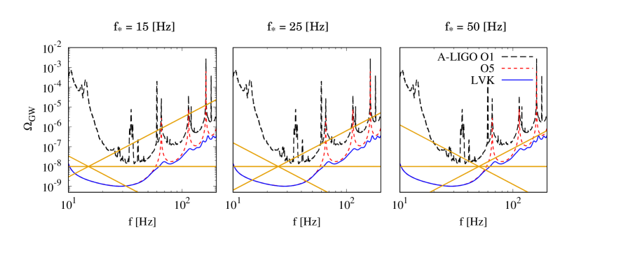
Figure 1: Comparison of the sensitivity curve and the GW spectra given in Eq. (2.4) for the cases with $f_{\ast}=15~{}{\rm Hz}$ (left), $25~{}{\rm Hz}$ (middle) and $50~{}{\rm Hz}$ (right). We show sensitivities of aLIGO O1 (black dashed), O5 (red dotted), and 4 detector network by aLIGO-aVirgo-KAGRA (LVK, blue solid). For the GW spectra (yellow solid), we fix the fiducial value of $\Omega_{\ast}$ at $10^{-8}$ and $n_{\rm GW1}$ and $n_{\rm GW2}$ take values on $-3,0,3$.

3.2 Parameterizing the GW spectrum

Although, as we discussed in Section 2, most sources of stochastic GW background have a broken power-law shape, a single observation may only be able to see a limited frequency range of the spectrum and may not cover the typical frequency at which the GW spectrum changes its scale dependence. In this case, the single power-law fit would be sufficient. Therefore, we make two types of analysis where we parametrize the GW spectrum as follows:

(i) Single power-law

$$\Omega_{\rm GW}(f)=\Omega_{\rm GW\ast}\left(\displaystyle\frac{f}{f_{\ast}}\right)^{n_{\rm GW}}\,.$$ (3.19)

(ii) Broken power-law

$$\Omega_{\rm GW}(f)=\begin{cases}&\Omega_{\rm GW\ast}\left(\displaystyle\frac{f}{f_{\ast}}\right)^{n_{\rm GW1}}\qquad\text{for}~{}~{}f<f_{\ast},\\ \\ &\Omega_{\rm GW\ast}\left(\displaystyle\frac{f}{f_{\ast}}\right)^{n_{\rm GW2}}\qquad\text{for}~{}~{}f>f_{\ast},\end{cases}$$ (3.20)

where $\Omega_{\rm GW\ast}$ is the amplitude at the reference frequency $f_{\ast}$.

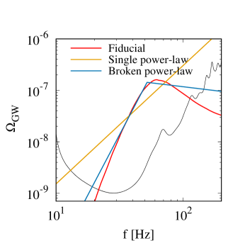
SNR $\delta\chi^{2}$ Single power-law 70.7 1440 Broken power-law 80.0 47.4 Fiducial 80.3 0

Figure 2: Left panel: Example of single and broken power-law fittings. The red line is the GW background generated by superradiant instabilities (taken from Fig. 2 of [125]). The yellow and blue lines are the best-fit spectra for single and broken power-law fits respectively. The black line shows the sensitivity curve of aLIGO-aVirgo-KAGRA. Right panel: SNR and $\delta\chi^{2}$ for the best-fit spectra, calculated assuming the aLIGO-aVirgo-KAGRA sensitivity.

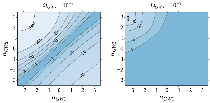
Figure 3: Contour plot of $\delta\chi^{2}|_{\rm diff}$ in the $n_{\rm GW1}$ – $n_{\rm GW2}$ plane, showing the difference of $\delta\chi^{2}$ between the single power-law fit, Eq. (3.19), and broken power-law fit, Eq. (3.20). The pivot frequency is fixed at $f_{\ast}=25$ Hz and the amplitude is taken as $\Omega_{\rm GW\ast}=10^{-8}$ in the left panel and $10^{-9}$ in the right panel. The specification of aLIGO-aVirgo-KAGRA is assumed.

Here we demonstrate how the choice of the template spectrum affects the value of $\delta\chi^{2}$, which describes the goodness of the fit. As an example, we take the case of GWs from superradiant instabilities (the most pessimistic case for $m_{s}=10^{-12.5}{\rm eV}$) [125]. In Fig. 2, the GW spectrum from the model, and the best-fit spectra for single and broken power-law templates are shown. In the right panel of Fig. 2, we tabulate the SNR expected for aLIGO-aVirgo-KAGRA and $\delta\chi^{2}$ for each case. We see that, when the fitting is performed with broken power-law templates, the value of SNR improves more than $10\%$ compared with the case fitted by the single power-law template. We also find the value of $\delta\chi^{2}$ significantly differs between single and broken power-law fits.

Let us extend the discussion to general cases with different values of the spectral indices $n_{\rm GW1}$ and $n_{\rm GW2}$. In Fig. 3, we show the contour plot of $\delta\chi^{2}|_{\rm diff}$ whose definition is

$$\delta\chi^{2}|_{\rm diff}\equiv\delta\chi^{2}|_{\textrm{single power-law}}-\delta\chi^{2}|_{\textrm{broken power-law}},$$ (3.21)

where $\delta\chi^{2}|_{\textrm{single power-law}}$ is calculated assuming that the fiducial spectrum is the broken-power spectrum with $n_{\rm GW1},n_{\rm GW2}$ and $f_{\ast}=25$ Hz and searching the best-fit spectrum using single power-law templates, while $\delta\chi^{2}|_{\textrm{broken power-law}}$ is calculated by fitting with broken power-law templates. Thus $\delta\chi^{2}|_{\rm diff}$ describes how much the fit gets worse when we use single power-law templates for broken power-law fiducial spectrum. Notice that, by definition, $\delta\chi^{2}|_{\textrm{broken power-law best-fit}}=0$. We show two cases where the amplitude is assumed as $\Omega_{\rm GW\ast}=10^{-8}$ and $10^{-9}$, and $\delta\chi^{2}$ is calculated by assuming the sensitivity of aLIGO-aVirgo-KAGRA. Note that the case with $n_{\rm GW1}=n_{\rm GW2}$ reduces to the case of a single power-law template, so $\delta\chi^{2}|_{\rm diff}$ is zero for $n_{\rm GW1}=n_{\rm GW2}$. We find that $\delta\chi^{2}|_{\rm diff}$ increases when the fiducial model deviates more from a single power-law case, i.e., as the broken power-law nature becomes more evident. This shows that we should use a broken power-law form for templates when the actual model has a break in the spectrum inside the frequency range to which the observation is sensitive. Therefore, we suggest that both single and broken power-law templates should be investigated when one analyzes a stochastic GW spectrum. It is also worth mentioning that $\delta\chi^{2}|_{\rm diff}$ increases when SNR is larger. As seen in the figure, $\delta\chi^{2}|_{\rm diff}$ for the case with a negative $n_{\rm GW1}$ and a positive $n_{\rm GW2}$ is larger than that for a positive $n_{\rm GW1}$ and a negative $n_{\rm GW2}$, since the former has a spectrum with a downward convex shape, which is detected with larger SNR for the same fiducial amplitude $\Omega_{\rm GW\ast}$. This tendency can be also seen by comparing the cases of different fiducial amplitude, $\Omega_{\rm GW\ast}=10^{-8}$ and $\Omega_{\rm GW\ast}=10^{-9}$.

4 Expected constraints from aLIGO-aVirgo-KAGRA and DECIGO

As we have seen in Sec. 2, stochastic backgrounds have different power-law dependence at high and low frequencies and the single power-law fit is not always a good approximation. We have introduced the broken power-law as the next step after the single power-law and, in Sec. 3, we demonstrated that the broken power-law template improves the fit. Note that, in some models, change of the spectral dependence is not sharp at $f_{*}$ and the broken power-law may not be the best choice of template. However, preparing precise templates is challenging for some models and, on top of that, we lose generality if we assume a specific model. Therefore here we investigate only the single and broken power-law cases as a simple setup.

Now we discuss to what extent we can probe the origin of GWs by looking at the shapes of the GW spectrum, which is characterized by the amplitude at the reference scale $f_{\ast}$ (this frequency also corresponds to the break of the power law for the broken power-law case) and spectral indices ($n_{\rm GW}$ for the single-power case, $n_{\rm GW1}$ and $n_{\rm GW2}$ for the broken power-law case). First, we discuss the analysis using the single power-law templates with aLIGO-aVirgo-KAGRA sensitivity, then the case of the broken power-law ones follows. Finally, we also present the results for DECIGO in Section 4.3.

4.1 Single power-law case

The single power-law templates have two free parameters to be determined: the amplitude $\Omega_{\rm GW\ast}$ (at the reference scale $f_{\ast}$) and the spectral index $n_{\rm GW}$. Let us first show the parameter space which will be accessible with the future experiment sensitivity. In Fig. 4, we show the expected SNR from aLIGO-aVirgo-KAGRA in the $\Omega_{\rm GW\ast}$–$n_{\rm GW}$ plane. Here the reference frequency is taken to be $f_{\ast}=25$ Hz, at which aLIGO O5 is most sensitive. The gray region in the figure is already excluded by aLIGO O1  [134] at 2$\sigma$ level. Note that this prediction changes depending on the fiducial frequency $f_{\ast}$. Since the sensitivity curve is not symmetric around $f_{\ast}=25$ Hz as seen in Fig. 1, contours of SNR are also slightly asymmetric. Also, since aLIGO O1 is most sensitive around $f\simeq 40$ Hz, a bluer spectrum tends to be excluded when we take $f_{\ast}=25$ Hz.

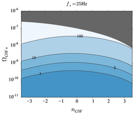
Figure 4: Contour plot representing the SNR in the $\Omega_{\rm GW\ast}$–$n_{\rm GW}$ plane for the case where the fiducial spectrum has single power-law shape. The reference frequency is taken to be $f_{\ast}=25$ Hz. The gray color represents the parameter space which is already constrained by aLIGO O1 at 2$\sigma$ level [134].

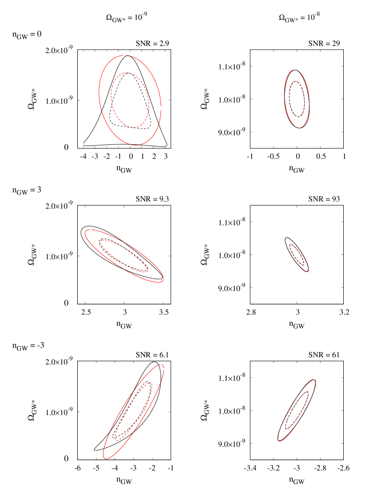
Figure 5: Expected constraints on parameters $\Omega_{\rm GW\ast}$ and $n_{\rm GW}$ for a single power-law case. We show 1$\sigma$ (dashed line) and 2$\sigma$ (solid line) limits estimated using the Fisher matrix analysis (red) and the $\chi^{2}$ analysis (black). Each panel corresponds to different fiducial values, $\Omega_{\rm GW\ast}=10^{-9}$ (left), $10^{-8}$ (right) and $n_{\rm GW}=0$ (top), $3$ (middle), $-3$ (bottom). The reference frequency is taken to be $f_{\ast}=25$ Hz.

Once we detect a GW background, we would be able to perform a parameter estimation and obtain the values of $\Omega_{\rm GW\ast}$ and $n_{\rm GW}$ with error bars. In Fig. 5, we demonstrate some examples of parameter constraints for different fiducial values of $\Omega_{\rm GW\ast}$ and $n_{\rm GW}$ assuming the aLIGO-aVirgo-KAGRA observation. See [128], for the first attempt to estimate errors on $\Omega_{\rm GW\ast}$ and $n_{\rm GW}$ for the analysis with a single power-law. We show two different contours; black curves represent results from the $\chi^{2}$ analysis with constant $\delta\chi^{2}$ slices at $\delta\chi^{2}=2.3$ ($1\sigma$) and $6.18$ ($2\sigma$), while red curves are those obtained by calculating the Fisher matrix under the assumption of a Gaussian likelihood shape around the reference parameter value. From the figure, we find that the shape of the likelihood function deviates from Gaussian when the SNR is low (left column, $\Omega_{\rm GW\ast}=10^{-9}$), while the Fisher prediction shows good agreement with the contours from $\chi^{2}$ analysis when the SNR is high (right column, $\Omega_{\rm GW\ast}=10^{-8}$). Therefore, by comparing the areas of the 1$\sigma$ allowed parameter space we may judge whether the Fisher matrix provides good estimate for predicting future constraints. Here we define the following quantity:

$$R\equiv\frac{\textrm{area of 1$\sigma$ allowed region obtained from the Fisher matrix analysis}}{\textrm{area of 1$\sigma$ allowed region obtained from the $\chi^{2}$ analysis}}.$$ (4.1)

We expect $R$ to become unity when the prediction from the Fisher matrix has a good agreement with that from the $\chi^{2}$ analysis. In Fig. 6, we show the ratio $R$ as a function of SNR for different fiducial values of the spectral index, $n_{\rm GW}=-3,0$ and $3$. Here raising the SNR is equivalent to increase the fiducial amplitude $\Omega_{\rm GW\ast}$. Although the tendency changes depending on the fiducial values of $n_{\rm GW}$, we find that $R$ is close to unity when SNR is larger than $\sim 5$, where we expect that we can safely adopt the Fisher matrix analysis.

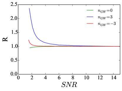
Figure 6: Comparison of the area of $1\sigma$ allowed region in the $\Omega_{\rm GW\ast}$–$n_{\rm GW}$ parameter space. The ratio $R$ is plotted as a function of SNR. Here the region of $\Omega_{\rm GW\ast}<0$ in the Fisher prediction is not included as the area.

Figure 7: Parameter space where $n_{\rm GW}$ can be determined with $\sigma_{n_{\rm GW}}<0.1$ (blue) and $<0.5$ (light blue) in the $n_{\rm GW}$–$\Omega_{\rm GW\ast}$ (left panel) and the $n_{\rm GW}$–SNR (right panel) planes. Here, $\Omega_{\rm GW\ast}$ is marginalized over. In the left panel, the reference frequency is taken at $f_{\ast}=25$ Hz.

Now we discuss to what extent we can determine the spectral index $n_{\rm GW}$ in future GW experiments. In general, the amplitude of GW strongly depends on the values of model parameters, especially for the cases of cosmological sources, while the spectral index $n_{\rm GW}$ does not, so that $n_{\rm GW}$ can be used to discriminate sources of the GW background. Therefore, the accuracy of the measurement of $n_{\rm GW}$ is of great interest. In Fig. 7, we show the parameter space where we can determine the value of $n_{\rm GW}$ with an accuracy of $\sigma_{n_{\rm GW}}<0.1$ (blue) and $<0.5$ (light blue) using aLIGO-aVirgo-KAGRA. It should be noted that when we show the result in the $n_{\rm GW}$–$\Omega_{\rm GW\ast}$ plane, the shape of the contours depends on $f_{\ast}$. For example, if one takes the reference frequency of $f_{\ast}\gg 25$ Hz ($f_{\ast}\ll 25$ Hz), the blue- (red-) tilted spectrum cannot be probed. On the other hand, when we take SNR as the vertical axis instead of $\Omega_{\rm GW\ast}$, it does not depend on $f_{\ast}$. This is because $f_{\ast}$ is a redundant parameter: Changing $f_{\ast}$ does not affect $n_{\rm GW}$ and can be compensated by changing $\Omega_{\rm GW\ast}$ and hence gives the same SNR (see Eqs. (3.9) and (3.10)). However, since the $n_{\rm GW}$–$\Omega_{\rm GW\ast}$ plane is easier to understand intuitively, we also show the results in the $n_{\rm GW}$–$\Omega_{\rm GW\ast}$ plane as well as in the $n_{\rm GW}$–SNR plane.

From the left panel, we find that, for $\Omega_{\rm GW\ast}>10^{-8}$ and $2\times 10^{-9}$, the spectral index $n_{\rm GW}$ can be respectively determined with the accuracy of $\sigma_{n_{\rm GW}}<0.1$ and $<0.5$ for all range of $n_{\rm GW}$ shown in the figure. We can also notice that, when the spectrum is more tilted, particularly when it is blue-tilted (i.e., $n_{\rm GW}>0$), $n_{\rm GW}$ can be better probed compared to the scale-invariant spectrum (i.e., $n_{\rm GW}=0$) for a fixed $\Omega_{\rm GW\ast}$. This is because the blue-tilted case is detectable with higher SNR for fixed $\Omega_{\rm GW\ast}$ and $f_{\ast}$, as seen in Fig. 4

We would like to note that the value of SNR changes proportional to $\Omega_{\rm GW\ast}$ as one can find by substituting Eq. (3.20) to Eq. (3.9), so the result here just scales as SNR $\propto\Omega_{\rm GW\ast}$ when one takes a different fiducial value of $\Omega_{\rm GW\ast}$ as long as the weak-signal approximation is valid. The same holds for the Fisher matrix prediction [128]. Thus, in the following results, the expected errors on the parameters can be scaled as $\sigma_{n_{\rm GW1,2}}\propto\Omega_{\rm GW\ast}^{-1}\propto{\rm SNR}^{-1}$.

4.2 Broken power-law case

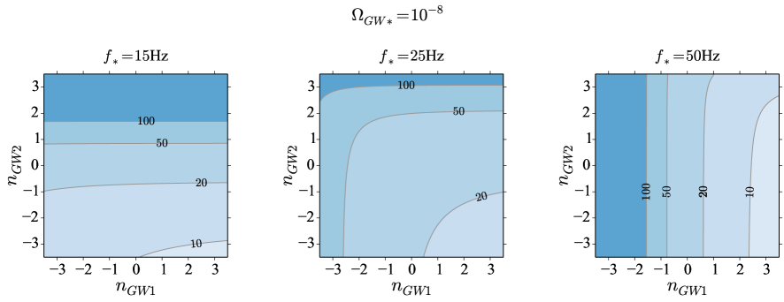
Figure 8: Detectability of the GWs for the broken power-law case. The contour plot of SNR in the $n_{\rm GW1}$–$n_{\rm GW2}$ plane for $\Omega_{\rm GW\ast}=10^{-8}$ is shown for different reference frequency $f_{\ast}=15~{}{\rm Hz}$ (left), $25~{}{\rm Hz}$ (middle) and $50~{}{\rm Hz}$ (right).

Next, we discuss the cases where we adopt the broken power-law form Eq. (3.20) as templates. First, in Fig. 8, we show contours of SNR for several values of $f_{\ast}$ by fixing $\Omega_{\rm GW\ast}=10^{-8}$ in the $n_{\rm GW1}$–$n_{\rm GW2}$ plane. One can notice that, the dependence on $n_{\rm GW1}$ and $n_{\rm GW2}$ change depending on the reference frequency. For example, the contours for the case of $f_{\ast}=50$ Hz are nearly vertical and $n_{\rm GW2}$ is irrelevant. This is because the number of frequency bands which is sensitive to $n_{\rm GW2}$ becomes smaller when $f_{\ast}$ is taken at higher frequency. A similar argument holds for the case of $f_{\ast}=15$ Hz in which $n_{\rm GW1}$ does not affect much the value of SNR and hence the contours are almost horizontal along the axis of $n_{\rm GW1}$.

Next, in Fig. 9, we show examples of parameter constraints in the $n_{\rm GW1}$–$n_{\rm GW2}$ plane assuming the aLIGO-aVirgo-KAGRA observation. Here, $\Omega_{\rm GW\ast}$ and $f_{\ast}$ are not marginalized. In the same way as Fig. 5, we compare predictions made by the $\chi^{2}$ and Fisher analyses. We show different sets of fiducial parameters $(n_{\rm GW1},n_{\rm GW2})=(3,-2)$, $(0,3)$ and $(-3,0)$, with different fiducial amplitude $\Omega_{\rm GW\ast}=10^{-8}$ (left) and $\Omega_{\rm GW\ast}=3\times 10^{-9}$ (right). The value of SNR for each fiducial parameters is also shown in the figure. As seen in Fig. 5, the smaller SNR, the more significant the deviation of the shape of the allowed region between the $\chi^{2}$ and Fisher analyses, which again indicates that the Fisher matrix analysis does not well describe expected constraints when SNR is small.

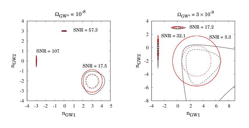
Figure 9: 1$\sigma$ (dashed line) and 2$\sigma$ (solid line) expected allowed region from the Fisher matrix (red) and the $\chi^{2}$ (black) analyses in the $n_{\rm GW1}$ – $n_{\rm GW2}$ plane for a broken power-law case. Different fiducial parameter cases $(n_{\rm GW1},n_{\rm GW2})=(3,-2),(0,3)$ and $(-3,0)$ are shown with the values of SNR for each case. Two panels show different fiducial value of $\Omega_{\rm GW\ast}=10^{-8}$ (left) and $3\times 10^{-9}$ (right). The fiducial reference frequency is taken to be $f_{\ast}=25$ Hz. Note that $\Omega_{\rm GW\ast}$ and $f_{\ast}$ are not marginalized in this figure.

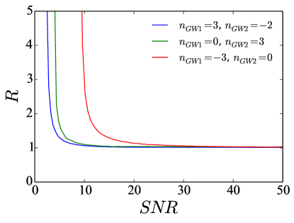
Figure 10: Ratio $R$ (defined in Eq. (4.1)) as a function of SNR. Cases with $(n_{\rm GW1},n_{\rm GW2})=(3,-2),(0,3)$ and $(-3,0)$ are shown.

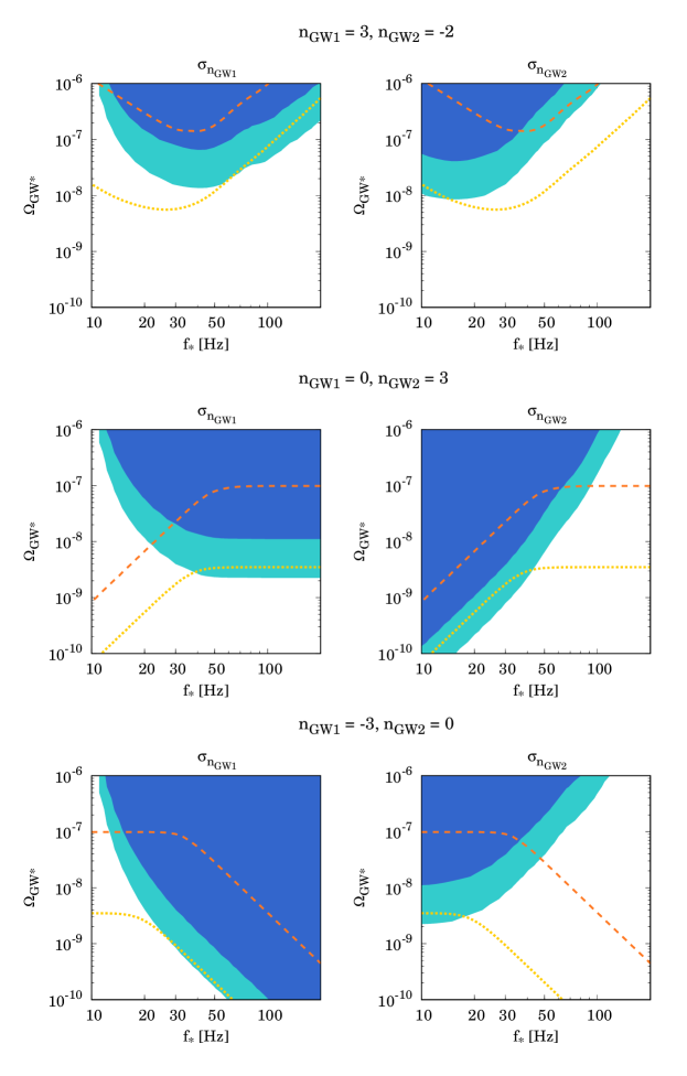
Figure 11: Regions with $\sigma_{n_{\rm GW1}}<0.1$ (blue) and $<0.5$ (light blue) are shown in the left panels, and those for $\sigma_{n_{\rm GW2}}<0.1$ and $<0.5$ are shown in the right panels in the $f_{\ast}$–$\Omega_{\rm GW\ast}$ parameter plane. The fiducial values of $(n_{\rm GW1},n_{\rm GW2})=(3,-2),(0,3)$ and $(-3,0)$ (from top to bottom) are shown. The region above the orange dashed line should be accessible with SNR $>2$ with the aLIGO O1 sensitivity, and the yellow dotted line indicates the accessible region by aLIGO-aVirgo-KAGRA with SNR $>10$.

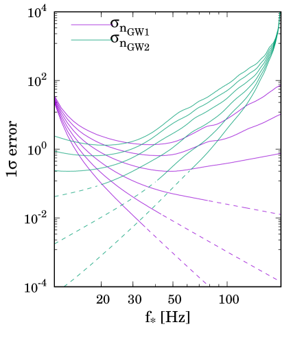
Figure 12: Plots of $1\sigma$ errors of the spectral indices, $\sigma_{n_{\rm GW1}}$ and $\sigma_{n_{\rm GW2}}$, as a function of $f_{\ast}$. Purple lines depict $\sigma_{n_{\rm GW1}}$ for the cases with $n_{\rm GW1}=5,3,1,-1,-3,-5$ from top to bottom and $n_{\rm GW2}=-4$ fixed. Green lines depict $\sigma_{n_{\rm GW2}}$ for the cases with $n_{\rm GW2}=5,3,1,-1,-3,-5$ from bottom to top and $n_{\rm GW1}=4$ fixed. Dashed lines correspond to the parameter regions which should be detectable with SNR $>2$ with the aLIGO O1 sensitivity. The fiducial value of $\Omega_{\rm GW\ast}$ is fixed to be $10^{-8}$.

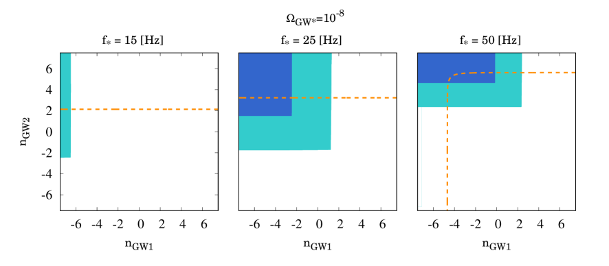
Figure 13: Regions satisfying both of $\sigma_{n_{\rm GW1}}<0.1~{}(0.5)$ and $\sigma_{n_{\rm GW2}}<0.1~{}(0.5)$ are shown with blue (light blue) for the cases with $f_{\ast}=15~{}{\rm Hz}$ (left), $25~{}{\rm Hz}$ (middle) and $50~{}{\rm Hz}$ (right). The amplitude is fixed as $\Omega_{\rm GW\ast}=10^{-8}$. Region above the orange dashed line should be accessible with SNR $>2$ with the aLIGO O1 sensitivity.

To quantify the validity of the Fisher matrix analysis, we again plot the ratio $R$ defined in Eq. (4.1) for some sets of $(n_{\rm GW1},n_{\rm GW2})$ in Fig. 10. We fix the reference frequency at $f_{\ast}=25$ Hz. In the same way as single power-law case, when the value of SNR is larger (say SNR $\gtrsim 10$), the ratio $R$ approaches unity, which means that the Fisher matrix analysis gives a good estimate. Note that the case of $(n_{\rm GW1},n_{\rm GW2})=(-3,0)$ is exceptional because in this case, the error contour is so elongated that the shape is almost one-dimensional as seen from Fig. 9 and the area ratio $R$ may not be a good indicator to check the validity of the Fisher matrix in this case. We also note here that the value of $R$ also depends on $f_{\ast}$. When we take the reference frequency away from $f_{\ast}=25$Hz at which aLIGO O5 is most sensitive, the uncertainty of $n_{\rm GW1}$ or $n_{\rm GW2}$ gets larger and the line would shift to the right.

In Fig. 11, the parameter space where we can determine $n_{\rm GW1}$ and $n_{\rm GW2}$ with $\sigma_{n_{\rm GW1}},\sigma_{n_{\rm GW2}}<0.1$ and $0.5$ for different fiducial values of $\Omega_{\rm GW\ast}$ and $f_{\ast}$ are shown in the $f_{\ast}$–$\Omega_{\rm GW\ast}$ plane, which represents how precisely we can determine the spectral indices with aLIGO-aVirgo-KAGRA. Here and in the following figures, Figs. 11, 12 and 13, other parameters are marginalized over in the Fisher analysis. The orange dashed line in the figure describes SNR $=2$ with the sensitivity of aLIGO O1 run. Thus, in the region above the orange dashed line, the GW background should be detectable with the O1 sensitivity if we perform a stochastic GW background search using broken power-law templates. We also show the region which can be accessible by aLIGO-aVirgo-KAGRA with SNR $>10$, whose lower bound is indicated by the yellow dotted line. From the left bottom panel of Fig. 11, one can easily notice that for larger values of $f_{\ast}$, negative $n_{\rm GW1}$ can be determined with high accuracy. This is because a broad range of the spectrum with $n_{\rm GW1}$ dependence is well inside the sensitivity curve when the reference frequency is high. Roughly speaking, errors of $n_{\rm GW1}$ get smaller when the experiment can measure the spectrum with $n_{\rm GW1}$ dependence in broad range of frequencies as large SNR is obtained by summing up contributions from each frequency bin. The same argument holds for $n_{\rm GW2}$.

The $f_{\ast}$ dependence can be clearly seen in Fig. 12 where 1$\sigma$ error is plotted as a function of $f_{\ast}$ for $n_{\rm GW1}=5,3,1,-1,-3,-5$ with $n_{\rm GW2}=-4$ being fixed (and $n_{\rm GW2}=5,3,1,-1,-3,-5$ with $n_{\rm GW1}=4$.). We can see the tendency that the error of $n_{\rm GW1}$ improves when $n_{\rm GW1}$ is more negative and $f_{\ast}$ is larger, while the error of $n_{\rm GW2}$ improves when $n_{\rm GW2}$ is more positive and $f_{\ast}$ is smaller, because they give larger SNR for fixed $\Omega_{\rm GW\ast}$. When $n_{\rm GW1}=5$ ($n_{\rm GW2}=-5$), we see that the error does not improve even when $f_{\ast}$ is high (low). This is because the spectral slope is so steep that the spectrum goes below the sensitivity curve quickly at low (high) frequencies and cannot increase the SNR.

In Fig. 13, the regions satisfying both $\sigma_{n_{\rm GW1}}<0.1~{}(0.5)$ and $\sigma_{n_{\rm GW2}}<0.1~{}(0.5)$ are depicted with dark blue (light blue) in the $n_{\rm GW1}$–$n_{\rm GW2}$ plane for $f_{\ast}=15$ Hz, $25$ Hz and $50$ Hz with $\Omega_{\rm GW\ast}=10^{-8}$ being fixed. The right edge of the rectangle is determined by $\sigma_{n_{\rm GW1}}<0.1~{}(0.5)$ and the lower edge of the rectangle is determined by $\sigma_{n_{\rm GW2}}<0.1~{}(0.5)$. The GW background should be detectable with aLIGO O1 run by SNR $>2$ in the region above the orange dashed line. As we would naively expect, we see that the GW spectrum can be well probed when the GW spectrum is convex downward (i.e., a negative $n_{\rm GW1}$ and a positive $n_{\rm GW2}$) since they give a large SNR for a fixed $\Omega_{\rm GW\ast}$. We can also see the tendency that, when we take a smaller $f_{\ast}$ (such as the case with $f_{\ast}=15~{}{\rm Hz}$), $n_{\rm GW2}$ can be easily probed. For larger $f_{\ast}$, we can better determine $n_{\rm GW1}$. Note that the case with $f_{\ast}=15~{}{\rm Hz}$ has a small parameter space where we can determine $n_{\rm GW1}$, because we have the low frequency cut off at $10$ Hz and the frequency range where $n_{\rm GW1}$ can be well probed is very narrow.

4.3 Expected constraints from DECIGO

Figure 14: Sensitivity curve for DECIGO (black solid). For comparison, we also plot the sensitivity curve of aLIGO-aVirgo-KAGRA (LVK) (blue dashed) as well as the spectra with $n_{\rm GW1}$ and $n_{\rm GW2}$ being assumed to be $-3,0$ and $3$ (yellow). We take $f_{\ast}=0.075~{}{\rm Hz}$ (left), $0.15~{}{\rm Hz}$ (middle) and $0.3~{}{\rm Hz}$ (right). The amplitude at $f_{\ast}$ is fixed to be $\Omega_{\rm GW\ast}=10^{-15}$.

We repeat the same analysis by assuming the specification of DECIGO in this section. The results are shown in Figs. 14–20. The tendencies are almost the same as those obtained for aLIGO-aVirgo-KAGRA, however, as seen from Fig. 14 where the sensitivity curve for DECIGO is shown, there are two important differences: (i) the frequency range sensitive to the signal, (ii) the sensitivity to $\Omega_{\rm GW\ast}$. DECIGO is sensitive to the frequency of $f\sim 0.1~{}{\rm Hz}$ and the sensitivity curve reaches $\Omega_{\rm GW\ast}\sim 2\times 10^{-16}$, which is about 7 orders of magnitude better than aLIGO-aVirgo-KAGRA.

Figure 15: Contours of SNR in the $n_{\rm GW}$–$\Omega_{\rm GW\ast}$ plane for a single power-law case expected from DECIGO. We take the reference frequency as $f_{\ast}=0.15~{}{\rm Hz}$, which is the most sensitive frequency for DECIGO.

Due to these differences, we take the reference frequency as (or close to) $f_{\ast}=0.15~{}{\rm Hz}$ in Figs. 15, 16 and 17, while $f_{\ast}$ taken to be ${\cal O}(10)$ Hz for aLIGO-aVirgo-KAGRA. Regarding the amplitude at the reference frequency $\Omega_{\rm GW\ast}$, we take it to be $\Omega_{\rm GW\ast}=10^{-15}$ in Fig. 19 and 20, while we mainly used $\Omega_{\rm GW\ast}=10^{-8}$ for aLIGO-aVirgo-KAGRA. Also since we assume the wide frequency range $10^{-3}$ – $10^{2}$ Hz for DECIGO, while $10$ – $200$ Hz for aLIGO-aVirgo-KAGRA, the result tends to be more sensitive to the change in the values of the spectral indices $n_{\rm GW1}$ and $n_{\rm GW2}$, since the amplitude of $\Omega_{\rm GW}(f)$ with tilt changes a lot when the frequency range is wide.

First, we consider the single power-law case in the same way as in Sec. 4.1. In Fig.15, we estimate SNR for a single power-law case with $f_{\ast}=0.15$ Hz in the $n_{\rm GW}$–$\Omega_{\rm GW\ast}$ plane. The figure clearly shows that DECIGO can probe much larger parameter space as it can detect GWs of $\Omega_{\rm GW\ast}\sim 10^{-15}$ with SNR $>10$ for any value of $n_{\rm GW}$. In Fig. 16, we show the parameter space where we can determine $n_{\rm GW}$ with $\sigma_{n_{\rm GW}}<0.1$ (orange) and $<0.5$ (yellow) using DECIGO. We find that SNR $>10$ is required to determine $n_{\rm GW}$, which is similar to the aLIGO-aVirgo-KAGRA case. If the stochastic GW background is detected by aLIGO-aVirgo-KAGRA, that would provide a prediction for the frequency range of DECIGO. For example, for $n_{\rm GW}=2/3$, which is the power index of the background generated by compact binary coalescence (see Sec. 2.2), the detection by aLIGO-aVirgo-KAGRA (LVK) would imply the amplitude at DECIGO as $\Omega_{\rm GW\ast}^{DECIGO}=\Omega_{\rm GW\ast}^{LVK}\left(\frac{0.15}{25}\right)^{2/3}\simeq 5.9\times 10^{-11}\left(\frac{\Omega_{\rm GW\ast}^{LVK}}{1.8\times 10^{-9}}\right)$, which should be detected by DECIGO with high SNR. Even for $n_{\rm GW}=3$, the amplitude at DECIGO becomes

$$\Omega_{\rm GW\ast}^{DECIGO}=3.9\times 10^{-16}\left(\frac{\Omega_{\rm GW\ast}^{LVK}}{1.8\times 10^{-9}}\right)\left(\frac{0.15{\rm Hz}}{25{\rm Hz}}\right)^{n_{\rm GW}-3},$$ (4.2)

which would be detected by DECIGO as shown in Fig. 16. Therefore, the detection of the stochastic GW background by DECIGO would be a consistency check of the detection by aLIGO-aVirgo-KAGRA.

Figure 16: Parameter space where $n_{\rm GW}$ can be determined in DECIGO with $\sigma_{n_{\rm GW}}<0.1$ (orange) and $<0.5$ (yellow) in the $n_{\rm GW}$–$\Omega_{\rm GW\ast}$ (left) and the $n_{\rm GW}$–SNR (right) planes. Here, $\Omega_{\rm GW\ast}$ is marginalized over. In the left panel, the reference frequency is taken at $f_{\ast}=0.15$ Hz.

Next, we consider the broken power-law case in the same way as in Sec. 4.2. In Fig. 17, we show the contours of SNR for several values of $f_{\ast}$ fixing $\Omega_{\rm GW\ast}=10^{-15}$ in the $n_{\rm GW1}$–$n_{\rm GW2}$ plane. We can find the same tendency with the case of aLIGO-aVirgo-KAGRA, but notice that the assumed value of $\Omega_{\rm GW\ast}$ is much smaller here. We can also see that the SNR is more sensitive to the change of $n_{\rm GW1}$ and $n_{\rm GW2}$ because of the wide frequency range $10^{-3}$ – $10^{2}$ Hz for DECIGO. In Fig. 18, we show the parameter space where the spectral indices can be determined with $\sigma_{n_{\rm GW1}}<0.1$ and $<0.5$ (left) and $\sigma_{n_{\rm GW2}}<0.1$ and $<0.5$ (right) in the $\Omega_{\rm GW\ast}$–$f_{\ast}$ plane. Here and in the following figures, Figs. 18, 19 and 20, other parameters are marginalized over in the analysis. For $(n_{\rm GW1},n_{\rm GW2})=(3,-2)$, which cannot be measured by aLIGO-aVirgo-KAGRA with $\Omega_{\rm GW\ast}=10^{-8}$, both indices can be measured with $\sigma_{n_{\rm GW1,2}}<0.1$ even with $\Omega_{\rm GW\ast}=10^{-13}$ for $0.03{\rm Hz}\lesssim f_{\ast}\lesssim 0.4$ Hz.

Fig. 19 shows $f_{\ast}$ dependence of 1$\sigma$ uncertainties of spectral indices, $\sigma_{n_{\rm GW1}}$ and $\sigma_{n_{\rm GW2}}$. In both figures, we find the same tendency with the case of aLIGO-aVirgo-KAGRA, but again the accessible amplitude and the frequency are different. Finally, in Fig. 20, we show parameter space where both $\sigma_{n_{\rm GW1}}<0.1(0.5)$ and $\sigma_{n_{\rm GW1}}<0.1(0.5)$ are satisfied in the $n_{\rm GW1}$–$n_{\rm GW2}$ plane. The upper panels may give impression that only small parameter space can be probed, but this is just because the fiducial amplitude assumed here, $\Omega_{\rm GW\ast}=10^{-15}$, is small. As seen in the lower panels, for $\Omega_{\rm GW\ast}=10^{-14}$, almost all the parameter space can be covered with DECIGO.

Figure 17: Detectability of DECIGO for the broken power-law case. The contour plot of SNR in the $n_{\rm GW1}$–$n_{\rm GW2}$ plane for $\Omega_{\rm GW\ast}=10^{-15}$ is shown for different reference frequency $f_{\ast}=0.075~{}{\rm Hz}$ (left), $0.15~{}{\rm Hz}$ (middle) and $0.3~{}{\rm Hz}$ (right).

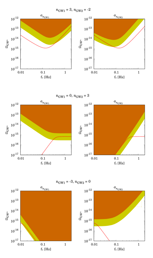
Figure 18: Errors on spectral indices expected in DECIGO are shown in the $\Omega_{\rm GW\ast}$–$f_{\ast}$ plane. The parameter space satisfying $\sigma_{n_{\rm GW1}}<0.1$ (orange) and $<0.5$ (yellow) are presented in the left panels, and those for $\sigma_{n_{\rm GW2}}$ are in the right panels. Cases with $(n_{\rm GW1},n_{\rm GW2})=(3,-2),(0,3)$ and $(-3,0)$ (from top to bottom) are shown. The red dotted line represents the accessible region by DECIGO with SNR $>10$.

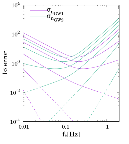
Figure 19: Plots of $1\sigma$ errors of the spectral indices, $\sigma_{n_{\rm GW1}}$ and $\sigma_{n_{\rm GW2}}$, as a function of $f_{\ast}$. Purple lines depict $\sigma_{n_{\rm GW1}}$ for the cases with $n_{\rm GW1}=5,3,1,-1,-3,-5$ from top to bottom and $n_{\rm GW2}=-4$ fixed. Green lines depict $\sigma_{n_{\rm GW2}}$ for the cases with $n_{\rm GW2}=5,3,1,-1,-3,-5$ from bottom to top and $n_{\rm GW1}=4$ fixed. Dashed lines correspond to the parameter range where the weak-signal approximation breaks down with ${\rm SNR}>100$. The fiducial value of $\Omega_{\rm GW\ast}$ is fixed to be $\Omega_{\rm GW\ast}=10^{-15}$.

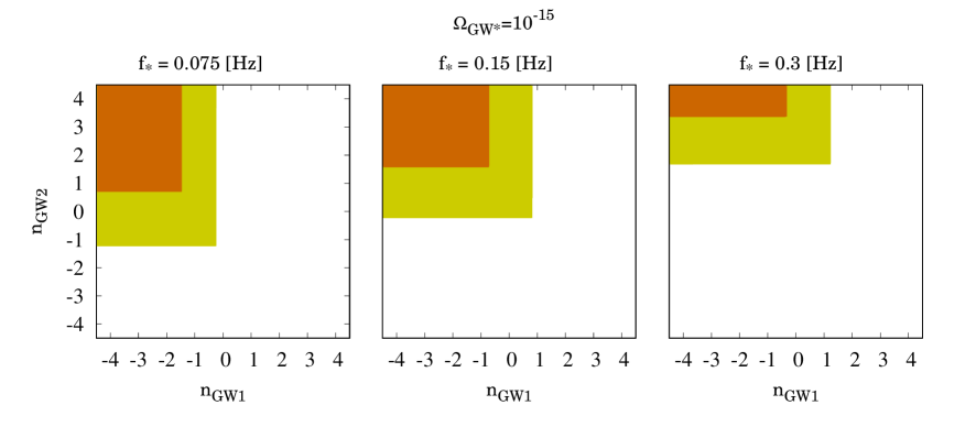
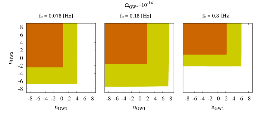
Figure 20: Regions satisfying both of $\sigma_{n_{\rm GW1}}<0.1~{}(0.5)$ and $\sigma_{n_{\rm GW2}}<0.1~{}(0.5)$ expected from DECIGO are shown with orange (yellow) for the cases with $f_{\ast}=0.075~{}{\rm Hz}$ (left), $0.15~{}{\rm Hz}$ (middle) and $0.3~{}{\rm Hz}$ (right). The fiducial amplitude is fixed to be $\Omega_{\rm GW\ast}=10^{-15}$ (upper panels) and $\Omega_{\rm GW\ast}=10^{-14}$ (lower panels).

5 Summary

Since the first detection of the GWs from the merger of a black hole binary [136], several GWs from the merger of binary black holes and neutron stars have been detected. We are now in the stage of a possible detection of the stochastic GW background from compact binary coalescence [115]. As we have seen in Sec. 2, there are lots of sources of stochastic GW background of cosmological origin as well as astrophysical ones. Most of the spectra of stochastic GW background cannot be fitted by a single power law, but rather they are better fitted by a broken power law.

In this paper, we have demonstrated the use of the broken power-law templates. We have also calculated the expected constraints on the parameters such as spectral indices by using the Fisher matrix analysis for both single and broken power-law templates, assuming the sensitivity of the future detector network of aLIGO-aVirgo-KAGRA and of a future detector DECIGO. For aLIGO-aVirgo-KAGRA, we have found that the spectral index of a single power-law template can be measured with $\sigma_{n_{\rm GW}}<0.1$ if $\Omega_{\rm GW\ast}>10^{-8}$ and that two indices of a broken power-law template with $f_{\ast}=25$ Hz (50 Hz) can be measured with an accuracy of $\sigma_{n_{\rm GW1,2}}<0.5$ for $n_{\rm GW1}\lesssim 1(2)$ and $n_{\rm GW2}\gtrsim-2(2)$ for $\Omega_{\rm GW\ast}>10^{-8}$. We have also estimated the required SNR in order for the Fisher matrix analysis to provide an accurate estimate of the parameters by comparing with the result from the $\chi^{2}$ analysis.

The accuracy would be improved significantly for DECIGO. The spectral index of a single power-law spectrum can be measured with $\sigma_{n_{\rm GW}}<0.1$ even for $\Omega_{\rm GW\ast}>10^{-15}$. For a broken power-law spectrum with $(n_{\rm GW1},n_{\rm GW2})=(3,-2)$, which cannot be measured by aLIGO-aVirgo-KAGRA with $\Omega_{\rm GW\ast}=10^{-8}$, both indexes can be measured with $\sigma_{n_{\rm GW1,2}}<0.1$ even with $\Omega_{\rm GW\ast}=10^{-13}$ for $0.03{\rm Hz}\lesssim f_{\ast}\lesssim 0.4$ Hz. With a possible detection of the stochastic background by aLIGO-aVirgo-KAGRA, the measurement by DECIGO could be used as a consistency check of the spectrum of the background.

The spectral indices would be useful to narrow down the sources of the background. Furthermore, it may also be possible to discriminate between a smooth background from cosmological sources and a discrete “popcorn-type” background such as the one from astrophysical sources and the one from the smooth stochastic background from the early universe sources (such as inflation) by measuring the non-Gaussianity of the GW data streams [137] or by the anisotropies of the spectrum [138]. By combining this information with the spectral indices studied in this paper, we can deepen our understandings of the Universe through the stochastic GW background.

References

- [1] A. A. Starobinsky, JETP Lett. 30, 682-685 (1979).
- [2] V. A. Rubakov, M. V. Sazhin, A. V. Veryaskin, Phys. Lett. B115, 189-192 (1982).
- [3] A. Kosowsky, M. S. Turner and R. Watkins, Phys. Rev. D 45, 4514 (1992)
- [4] A. Kosowsky, M. S. Turner and R. Watkins, Phys. Rev. Lett. 69, 2026 (1992).
- [5] A. Kosowsky and M. S. Turner, Phys. Rev. D 47, 4372 (1993) [arXiv:astro-ph/9211004].
- [6] M. Kamionkowski, A. Kosowsky and M. S. Turner, Phys. Rev. D 49, 2837 (1994) [arXiv:astro-ph/9310044].
- [7] M. Hindmarsh, S. J. Huber, K. Rummukainen and D. J. Weir, Phys. Rev. Lett. 112, 041301 (2014) [arXiv:1304.2433 [hep-ph]].
- [8] S. Y. Khlebnikov, I. I. Tkachev, Phys. Rev. D56, 653-660 (1997). [hep-ph/9701423].
- [9] A. Vilenkin, Phys. Rev. D 23, 852 (1981).
- [10] T. Vachaspati, A. Vilenkin, Phys. Rev. D31, 3052 (1985).
- [11] T. Damour and A. Vilenkin, Phys. Rev. Lett. 85, 3761 (2000) [arXiv:gr-qc/0004075].
- [12] L. M. Krauss, Phys. Lett. B 284, 229 (1992).
- [13] E. Fenu, D. G. Figueroa, R. Durrer and J. Garcia-Bellido, JCAP 0910, 005 (2009) [arXiv:0908.0425 [astro-ph.CO]].
- [14] D. Meacher et al., Phys. Rev. D 92, no. 6, 063002 (2015) [arXiv:1506.06744 [astro-ph.HE]].
- [15] A. J. Farmer and E. S. Phinney, Mon. Not. Roy. Astron. Soc. 346, 1197 (2003) [astro-ph/0304393].
- [16] A. Buonanno, G. Sigl, G. G. Raffelt, H. -T. Janka, E. Muller, Phys. Rev. D72, 084001 (2005). [astro-ph/0412277].
- [17] K. Crocker, T. Prestegard, V. Mandic, T. Regimbau, K. Olive and E. Vangioni, Phys. Rev. D 95, no. 6, 063015 (2017) [arXiv:1701.02638 [astro-ph.CO]].
- [18] V. Ferrari, S. Matarrese and R. Schneider, Mon. Not. Roy. Astron. Soc. 303, 258 (1999) [astro-ph/9806357].
- [19] T. Regimbau and J. A. de Freitas Pacheco, Astron. Astrophys. 447, 1 (2006) [astro-ph/0509880].
- [20] N. Seto, S. Kawamura and T. Nakamura, Phys. Rev. Lett. 87, 221103 (2001) [astro-ph/0108011].
- [21] S. Kawamura et al., Class. Quant. Grav. 28, 094011 (2011).
- [22] S. Bose, Phys. Rev. D 71, 082001 (2005) [astro-ph/0504048].
- [23] P. Binetruy, A. Bohe, C. Caprini and J. F. Dufaux, JCAP 1206, 027 (2012) [arXiv:1201.0983 [gr-qc]].
- [24] C. Caprini and D. G. Figueroa, arXiv:1801.04268 [astro-ph.CO].
- [25] R. Apreda, M. Maggiore, A. Nicolis and A. Riotto, Nucl. Phys. B 631, 342 (2002) [gr-qc/0107033].
- [26] C. Grojean and G. Servant, Phys. Rev. D 75, 043507 (2007) [hep-ph/0607107].
- [27] R. Jinno, S. Lee, H. Seong and M. Takimoto, JCAP 1711, 050 (2017) [arXiv:1708.01253 [hep-ph]].
- [28] D. Croon, V. Sanz and G. White, arXiv:1806.02332 [hep-ph].
- [29] C. Caprini, R. Durrer and G. Servant, Phys. Rev. D 77, 124015 (2008) [arXiv:0711.2593 [astro-ph]].
- [30] S. J. Huber and T. Konstandin, JCAP 0809, 022 (2008) [arXiv:0806.1828 [hep-ph]].
- [31] C. Caprini et al., JCAP 1604, no. 04, 001 (2016) [arXiv:1512.06239 [astro-ph.CO]].
- [32] C. Caprini, R. Durrer, T. Konstandin and G. Servant, Phys. Rev. D 79, 083519 (2009) [arXiv:0901.1661 [astro-ph.CO]].
- [33] R. Jinno and M. Takimoto, Phys. Rev. D 95, no. 2, 024009 (2017) doi:10.1103/PhysRevD.95.024009 [arXiv:1605.01403 [astro-ph.CO]].
- [34] R. Jinno and M. Takimoto, arXiv:1707.03111 [hep-ph].
- [35] C. Caprini, R. Durrer and G. Servant, JCAP 0912, 024 (2009) [arXiv:0909.0622 [astro-ph.CO]].
- [36] M. Hindmarsh, S. J. Huber, K. Rummukainen and D. J. Weir, Phys. Rev. D 92, no. 12, 123009 (2015) [arXiv:1504.03291 [astro-ph.CO]].
- [37] M. Hindmarsh, S. J. Huber, K. Rummukainen and D. J. Weir, Phys. Rev. D 96, no. 10, 103520 (2017) [arXiv:1704.05871 [astro-ph.CO]].
- [38] R. Allahverdi, R. Brandenberger, F. Y. Cyr-Racine and A. Mazumdar, Ann. Rev. Nucl. Part. Sci. 60, 27 (2010) [arXiv:1001.2600 [hep-th]].
- [39] M. A. Amin, M. P. Hertzberg, D. I. Kaiser and J. Karouby, Int. J. Mod. Phys. D 24, 1530003 (2014) [arXiv:1410.3808 [hep-ph]].
- [40] J. F. Dufaux, D. G. Figueroa and J. Garcia-Bellido, Phys. Rev. D 82 (2010) 083518 doi:10.1103/PhysRevD.82.083518 [arXiv:1006.0217 [astro-ph.CO]].
- [41] A. Tranberg, S. Tähtinen and D. J. Weir, JCAP 1804, no. 04, 012 (2018) doi:10.1088/1475-7516/2018/04/012 [arXiv:1706.02365 [hep-ph]].
- [42] P. Adshead, J. T. Giblin and Z. J. Weiner, arXiv:1805.04550 [astro-ph.CO].
- [43] D. G. Figueroa and F. Torrenti, JCAP 1710, no. 10, 057 (2017) [arXiv:1707.04533 [astro-ph.CO]].
- [44] J. Garcia-Bellido and D. G. Figueroa, Phys. Rev. Lett. 98, 061302 (2007) [astro-ph/0701014].
- [45] J. F. Dufaux, G. Felder, L. Kofman and O. Navros, JCAP 0903, 001 (2009) [arXiv:0812.2917 [astro-ph]].
- [46] T. Damour and A. Vilenkin, Phys. Rev. D 64, 064008 (2001) [arXiv:gr-qc/0104026].
- [47] T. Damour and A. Vilenkin, Phys. Rev. D 71, 063510 (2005) [arXiv:hep-th/0410222].
- [48] X. Siemens, V. Mandic and J. Creighton, Phys. Rev. Lett. 98, 111101 (2007) [arXiv:astro-ph/0610920].
- [49] M. R. DePies and C. J. Hogan, Phys. Rev. D 75, 125006 (2007) [arXiv:astro-ph/0702335];
- [50] S. Olmez, V. Mandic and X. Siemens, Phys. Rev. D 81, 104028 (2010) [arXiv:1004.0890 [astro-ph.CO]].
- [51] S. A. Sanidas, R. A. Battye and B. W. Stappers, Phys. Rev. D 85, 122003 (2012) [arXiv:1201.2419 [astro-ph.CO]].
- [52] S. A. Sanidas, R. A. Battye and B. W. Stappers, Astrophys. J. 764, 108 (2013) [arXiv:1211.5042 [astro-ph.CO]].
- [53] S. Kuroyanagi, K. Miyamoto, T. Sekiguchi, K. Takahashi and J. Silk, Phys. Rev. D 86, 023503 (2012) [arXiv:1202.3032 [astro-ph.CO]].
- [54] S. Kuroyanagi, K. Miyamoto, T. Sekiguchi, K. Takahashi and J. Silk, Phys. Rev. D 87, no. 2, 023522 (2013) [Phys. Rev. D 87, no. 6, 069903 (2013)] [arXiv:1210.2829 [astro-ph.CO]].
- [55] L. Sousa and P. P. Avelino, Phys. Rev. D 88, no. 2, 023516 (2013) [arXiv:1304.2445 [astro-ph.CO]].
- [56] J. J. Blanco-Pillado and K. D. Olum, Phys. Rev. D 96, no. 10, 104046 (2017) [arXiv:1709.02693 [astro-ph.CO]].
- [57] C. Ringeval and T. Suyama, JCAP 1712, no. 12, 027 (2017) [arXiv:1709.03845 [astro-ph.CO]].
- [58] M. Kawasaki, K. Miyamoto and K. Nakayama, Phys. Rev. D 81, 103523 (2010) [arXiv:1002.0652 [astro-ph.CO]].
- [59] Y. Matsui, K. Horiguchi, D. Nitta and S. Kuroyanagi, JCAP 1611, no. 11, 005 (2016) [arXiv:1605.08768 [astro-ph.CO]].
- [60] M. Gleiser and R. Roberts, Phys. Rev. Lett. 81, 5497 (1998) [astro-ph/9807260].
- [61] T. Hiramatsu, M. Kawasaki and K. Saikawa, JCAP 1402, 031 (2014) [arXiv:1309.5001 [astro-ph.CO]].
- [62] M. Kawasaki and K. Saikawa, JCAP 1109, 008 (2011) [arXiv:1102.5628 [astro-ph.CO]].
- [63] K. Saikawa, Universe 3, no. 2, 40 (2017) [arXiv:1703.02576 [hep-ph]].
- [64] K. Jones-Smith, L. M. Krauss and H. Mathur, Phys. Rev. Lett. 100, 131302 (2008) [arXiv:0712.0778 [astro-ph]].
- [65] J. T. Giblin, Jr., L. R. Price, X. Siemens and B. Vlcek, JCAP 1211, 006 (2012) [arXiv:1111.4014 [astro-ph.CO]].
- [66] D. G. Figueroa, M. Hindmarsh and J. Urrestilla, Phys. Rev. Lett. 110, no. 10, 101302 (2013) [arXiv:1212.5458 [astro-ph.CO]].
- [67] S. Kuroyanagi, T. Hiramatsu and J. Yokoyama, JCAP 1602, no. 02, 023 (2016) [arXiv:1509.08264 [astro-ph.CO]].
- [68] C. Caprini and R. Durrer, Phys. Rev. D 65, 023517 (2001) [astro-ph/0106244].
- [69] C. Caprini and R. Durrer, Phys. Rev. D 74, 063521 (2006) [astro-ph/0603476].
- [70] A. Neronov and I. Vovk, Science 328, 73 (2010) [arXiv:1006.3504 [astro-ph.HE]].
- [71] M. S. Turner and L. M. Widrow, Phys. Rev. D 37, 2743 (1988).
- [72] B. Ratra, Astrophys. J. 391, L1 (1992).
- [73] T. Vachaspati, Phys. Lett. B 265, 258 (1991).
- [74] K. Enqvist and P. Olesen, Phys. Lett. B 319, 178 (1993) [hep-ph/9308270].
- [75] M. S. Turner, M. J. White and J. E. Lidsey, Phys. Rev. D 48, 4613 (1993) [astro-ph/9306029].
- [76] K. Nakayama, S. Saito, Y. Suwa and J. Yokoyama, JCAP 0806, 020 (2008) [arXiv:0804.1827 [astro-ph]].
- [77] K. Nakayama and J. Yokoyama, JCAP 1001, 010 (2010) [arXiv:0910.0715 [astro-ph.CO]].
- [78] S. Kuroyanagi, K. Nakayama and S. Saito, Phys. Rev. D 84, 123513 (2011) [arXiv:1110.4169 [astro-ph.CO]].
- [79] S. Kuroyanagi, T. Takahashi and S. Yokoyama, JCAP 1502, 003 (2015) [arXiv:1407.4785 [astro-ph.CO]].
- [80] M. Giovannini, Phys. Rev. D 58, 083504 (1998) [hep-ph/9806329].
- [81] P. J. E. Peebles and A. Vilenkin, Phys. Rev. D 59, 063505 (1999) [astro-ph/9810509].
- [82] M. Giovannini, Phys. Rev. D 60, 123511 (1999) [astro-ph/9903004].
- [83] M. Giovannini, Class. Quant. Grav. 16, 2905 (1999) [hep-ph/9903263].
- [84] H. Tashiro, T. Chiba and M. Sasaki, Class. Quant. Grav. 21, 1761 (2004) [gr-qc/0307068].
- [85] M. Giovannini, Class. Quant. Grav. 26, 045004 (2009) [arXiv:0807.4317 [astro-ph]].
- [86] L. Senatore, E. Silverstein and M. Zaldarriaga, JCAP 1408, 016 (2014) [arXiv:1109.0542 [hep-th]].
- [87] J. L. Cook and L. Sorbo, Phys. Rev. D 85, 023534 (2012) Erratum: [Phys. Rev. D 86, 069901 (2012)] [arXiv:1109.0022 [astro-ph.CO]].
- [88] N. Bartolo et al., JCAP 1612, no. 12, 026 (2016) [arXiv:1610.06481 [astro-ph.CO]].
- [89] P. Adshead, E. Martinec and M. Wyman, Phys. Rev. D 88, no. 2, 021302 (2013) [arXiv:1301.2598 [hep-th]].
- [90] P. Adshead, E. Martinec and M. Wyman, JHEP 1309, 087 (2013) [arXiv:1305.2930 [hep-th]].
- [91] E. Dimastrogiovanni, M. Fasiello and T. Fujita, JCAP 1701, no. 01, 019 (2017) [arXiv:1608.04216 [astro-ph.CO]].
- [92] T. Fujita, R. Namba and Y. Tada, Phys. Lett. B 778, 17 (2018) [arXiv:1705.01533 [astro-ph.CO]].
- [93] B. Thorne, T. Fujita, M. Hazumi, N. Katayama, E. Komatsu and M. Shiraishi, Phys. Rev. D 97, no. 4, 043506 (2018) [arXiv:1707.03240 [astro-ph.CO]].
- [94] I. Ben-Dayan, JCAP 1609, no. 09, 017 (2016) [arXiv:1604.07899 [astro-ph.CO]].
- [95] N. Barnaby and M. Peloso, Phys. Rev. Lett. 106, 181301 (2011) [arXiv:1011.1500 [hep-ph]].
- [96] L. Sorbo, JCAP 1106, 003 (2011) [arXiv:1101.1525 [astro-ph.CO]].
- [97] N. Barnaby, E. Pajer and M. Peloso, Phys. Rev. D 85, 023525 (2012) [arXiv:1110.3327 [astro-ph.CO]].
- [98] D. Baumann, P. J. Steinhardt, K. Takahashi and K. Ichiki, Phys. Rev. D 76, 084019 (2007) [hep-th/0703290].
- [99] H. Assadullahi and D. Wands, Phys. Rev. D 79, 083511 (2009) [arXiv:0901.0989 [astro-ph.CO]].
- [100] R. Saito and J. Yokoyama, Phys. Rev. Lett. 102, 161101 (2009) Erratum: [Phys. Rev. Lett. 107, 069901 (2011)] [arXiv:0812.4339 [astro-ph]].
- [101] M. Kawasaki, N. Kitajima and S. Yokoyama, JCAP 1308, 042 (2013) doi:10.1088/1475-7516/2013/08/042 [arXiv:1305.4464 [astro-ph.CO]].
- [102] J. R. Espinosa, D. Racco and A. Riotto, arXiv:1804.07732 [hep-ph].
- [103] K. Kohri and T. Terada, arXiv:1804.08577 [gr-qc].
- [104] L. Alabidi, K. Kohri, M. Sasaki and Y. Sendouda, JCAP 1305, 033 (2013) [arXiv:1303.4519 [astro-ph.CO]].
- [105] L. Alabidi, K. Kohri, M. Sasaki and Y. Sendouda, JCAP 1209, 017 (2012) [arXiv:1203.4663 [astro-ph.CO]].
- [106] A. Buonanno, M. Maggiore and C. Ungarelli, Phys. Rev. D 55, 3330 (1997) [gr-qc/9605072].
- [107] V. Mandic and A. Buonanno, Phys. Rev. D 73, 063008 (2006) [astro-ph/0510341].
- [108] M. Gasperini, JCAP 1612, no. 12, 010 (2016) [arXiv:1606.07889 [gr-qc]].
- [109] M. Gasperini and M. Giovannini, Phys. Lett. B 282, 36 (1992).
- [110] R. Brustein, M. Gasperini, M. Giovannini and G. Veneziano, Phys. Lett. B 361, 45 (1995)
- [111] R. Schneider, S. Marassi and V. Ferrari, Class. Quant. Grav. 27, 194007 (2010) [arXiv:1005.0977 [astro-ph.CO]].
- [112] X. J. Zhu, E. Howell, T. Regimbau, D. Blair and Z. H. Zhu, Astrophys. J. 739, 86 (2011) [arXiv:1104.3565 [gr-qc]].
- [113] X. J. Zhu, E. J. Howell, D. G. Blair and Z. H. Zhu, Mon. Not. Roy. Astron. Soc. 431, no. 1, 882 (2013) [arXiv:1209.0595 [gr-qc]].
- [114] B. P. Abbott et al. [LIGO Scientific and Virgo Collaborations], Phys. Rev. Lett. 116, no. 13, 131102 (2016) [arXiv:1602.03847 [gr-qc]].
- [115] B. P. Abbott et al. [LIGO Scientific and Virgo Collaborations], Phys. Rev. Lett. 120, 091101 (2018) [arXiv:1710.05837 [gr-qc]].
- [116] B. P. Abbott et al. [LIGO Scientific and Virgo Collaborations], Phys. Rev. Lett. 119, no. 16, 161101 (2017) [arXiv:1710.05832 [gr-qc]].
- [117] B. Mueller, H. T. Janka and A. Marek, Astrophys. J. 766, 43 (2013) [arXiv:1210.6984 [astro-ph.SR]].
- [118] C. D. Ott et al., Astrophys. J. 768, 115 (2013) [arXiv:1210.6674 [astro-ph.HE]].
- [119] T. Kuroda, T. Takiwaki and K. Kotake, Phys. Rev. D 89, no. 4, 044011 (2014) [arXiv:1304.4372 [astro-ph.HE]].
- [120] X. J. Zhu, X. L. Fan and Z. H. Zhu, Astrophys. J. 729, 59 (2011) [arXiv:1102.2786 [astro-ph.CO]].
- [121] N. Andersson, Astrophys. J. 502, 708 (1998) [gr-qc/9706075].
- [122] J. L. Friedman and S. M. Morsink, Astrophys. J. 502, 714 (1998) [gr-qc/9706073].
- [123] J. L. Friedman, J. R. Ipser and L. Parker, Phys. Rev. Lett. 62, 3015 (1989).
- [124] S. Marassi, R. Ciolfi, R. Schneider, L. Stella and V. Ferrari, Mon. Not. Roy. Astron. Soc. 411, 2549 (2011) [arXiv:1009.1240 [astro-ph.CO]].
- [125] R. Brito, S. Ghosh, E. Barausse, E. Berti, V. Cardoso, I. Dvorkin, A. Klein and P. Pani, Phys. Rev. Lett. 119, no. 13, 131101 (2017) [arXiv:1706.05097 [gr-qc]].
- [126] H. Yoshino and H. Kodama, PTEP 2014, 043E02 (2014) [arXiv:1312.2326 [gr-qc]].
- [127] B. Allen and J. D. Romano, Phys. Rev. D 59, 102001 (1999) [arXiv:gr-qc/9710117].
- [128] N. Seto, Phys. Rev. D 73, 063001 (2006) [arXiv:gr-qc/0510067].
- [129] A. Nishizawa, A. Taruya, K. Hayama, S. Kawamura and M. a. Sakagami, Phys. Rev. D 79, 082002 (2009) [arXiv:0903.0528 [astro-ph.CO]].
- [130] H. Kudoh, A. Taruya, T. Hiramatsu and Y. Himemoto, Phys. Rev. D 73, 064006 (2006) [gr-qc/0511145].
- [131] B. P. Abbott et al. [LIGO Scientific and VIRGO Collaborations], Living Rev. Rel. 19, 1 (2016) [arXiv:1304.0670 [gr-qc]].
- [132] https://dcc.ligo.org/LIGO-P1200087/public
- [133] S. Kuroyanagi, T. Chiba and N. Sugiyama, Phys. Rev. D 83, 043514 (2011) [arXiv:1010.5246 [astro-ph.CO]].
- [134] B. P. Abbott et al. [LIGO Scientific and Virgo Collaborations], Phys. Rev. Lett. 118, no. 12, 121101 (2017) Erratum: [Phys. Rev. Lett. 119, no. 2, 029901 (2017)] [arXiv:1612.02029 [gr-qc]].
- [135] H. Audley et al. [LISA Collaboration], arXiv:1702.00786 [astro-ph.IM].
- [136] B. P. Abbott et al. [LIGO Scientific and Virgo Collaborations], Phys. Rev. Lett. 116, no. 6, 061102 (2016) [arXiv:1602.03837 [gr-qc]].
- [137] N. Seto, Astrophys. J. 683, L95 (2008) [arXiv:0807.1151 [astro-ph]].
- [138] G. Cusin, I. Dvorkin, C. Pitrou and J. P. Uzan, arXiv:1803.03236 [astro-ph.CO].