Modular-value-based metrology with spin coherent pointers

Abstract

Modular values are quantities that described by pre- and postselected states of quantum systems like weak values but are different from them: The associated interaction is not necessary to be weak. We discuss an optimal modular-value-based measurement with a spin coherent pointer: A quantum system is exposed to a field in which strength is to be estimated through its modular value. We consider two cases, with a two-dimensional and a higher-dimensional pointer, and evaluate the quantum Fisher information. The modular-value-based measurement has no merit in the former case, while its sensitivity can be enhanced in the latter case. We also consider the pointer under a phase-flip error. Our study should motivate researchers to apply the modular-value-based measurements for quantum metrology.

Introduction.—In the concept of quantum sensing, a physical quantity on a small scale can be measured indirectly via a quantum system, a quantum property, or a quantum phenomenon Degen89 . The principle of measurements is (i) preparing quantum systems, hereafter called sensors, of which number is $L$, (ii) exposing to a field of which strength is to be measured for a period of $t$, and (iii) obtaining a state change before and after the exposure. The change is a measure of the strength of the field. This procedure is repeated $T/t$ times in a total measurement time $T$. If the sensors are independent, the effective total measurement number $N$ is given as $N=LT/t$. For fixed $T$ and $t$, the uncertainty of the estimation is proportional to $1/\sqrt{L}$, which is known as the standard quantum limit or the shot noise limit Matsuzaki84 ; Pezze102 ; Huelga79 ; Itano47 . However, if the uncertainty scales as $1/L$ then it is called the Heisenberg limit Zwierz105 which is a fundamental limit.

There have been a number of attempts to improve measurement protocols to overcome the standard quantum limit. One of the pioneering attempts is to employ squeezed states to reduce noises Wineland46 ; Wineland50 ; Giovannetti306 . The entanglement is also a resource for defeating the standard quantum limit Giovannetti306 ; Giovannetti96 ; Huelga79 ; Pezze102 ; Jones342 ; Simmons82 . For example, Jones et al. have used $\it NOON$ states Jones342 ; Simmons82 . Zaiser et al. have claimed that the sensitivity can be significantly enhanced by using a quantum memory Zaiser7 . Matsuzaki et al. have proposed a protocol with a teleportation Matsuzaki120 .

These studies focused on sensors exposed to a field. We, here, draw attention a method how the sensors are measured. One approach in this direction is employing a weak value Aha60 ; Aha2005 ; Kofman520 ; Dressel86 . Measurements with weak values had been expected to enhance the sensitivity Alves95 ; Zhang114 ; Alves91 ; Tanaka88 ; Knee87 ; Knee4 , but it turned out that they can only reach the standard quantum limit Alves95 ; Zhang114 ; Alves91 ; Tanaka88 ; Knee87 ; Knee4 . The measurements with weak values, however, can be dramatically improved when sensors are entangled Pang113 ; Pang92 . Furthermore, by employing non-classical pointer states, the sensitivity can reach the Heisenberg limit Zhang114 ; Pang115 ; Jordan2 .

In this Letter, we discuss modular-value-based measurements Kedem105 ; Ho380 ; Ho95 ; Ho59 ; Ho97 with spin-$j$ coherent pointers Amiet24 ; Fabian93 . They are different from the weak-value-based ones and can allow arbitrary strength interactions between the pointers and sensors. The pointer may be considered as a measurement device for extracting the field information from the sensors. In order to evaluate the sensitivity, we focus on the quantum Fisher information contained in the Cramér-Rao inequality Zwierz105 ; Hofmann86 ; Braunstein72 ; Rao . Its maximum provides the lower bound on the sensitivity for measuring the field. In this Letter, $L$ is fixed and we compare the Fisher information of the measurements under various conditions. We first examine a measurement with a $j=\frac{1}{2}$ (qubit) pointer and then move our attention to that with a $j\geq 1$ pointer. We also consider the case when the qubit pointer is under a phase-flip error Nielsen .

Modular-value-based measurement.— We assume that the sensor exposed to a field is a qubit and that its initial state is $|\psi_{i}\rangle=\frac{1}{\sqrt{2}}(|0\rangle+|1\rangle)$ which evolves to $|\psi_{i}(\omega)\rangle=\frac{1}{\sqrt{2}}(|0\rangle+e^{-i\omega t}|1\rangle)$ during a period $t$. $\omega$ is a measure of the field strength to be estimated. We prepare the pointer in a spin-$j$ coherent state

$$|\xi\rangle=\sum_{m=-j}^{j}\sqrt{{2j\choose j+m}}\Bigl{(}\cos\frac{\theta}{2}\Bigr{)}^{j+m}\Bigl{(}\sin\frac{\theta}{2}e^{-i\varphi}\Bigr{)}^{j-m}|j,m\rangle$$ (1)

in spherical representation Amiet24 ; Fabian93 , where $\theta\in[0,\pi]$ and $\varphi\in[0,2\pi]$. $|j,m\rangle$ is the standard angular momentum basis, for a fixed $j$, $m\in[-j,+j]$.

The interaction Hamiltonian between the sensor and the pointer is assumed to be $\hat{H}=g(\tau){\sigma}_{z}\otimes|j,+j\rangle\langle j,+j|$. After the interaction during $\tau=0\sim\tau_{0}$, the joint state of the sensor-pointer yields

$$|\Psi(\omega)\rangle=\dfrac{1}{\sqrt{2}}\Bigl{(}|0\rangle\otimes|\xi_{+}\rangle+e^{-i\omega t}|1\rangle\otimes|\xi_{-}\rangle\Bigr{)},$$ (2)

where $|\xi_{\pm}\rangle=\exp(\mp ig|j,+j\rangle\langle j,+j|)|\xi\rangle$ and $g=\int_{0}^{\tau_{0}}g(\tau)d\tau$ is the coupling strength. After postselecting the sensor onto a final state $|\psi_{f}\rangle=\cos\frac{\phi}{2}|0\rangle+\sin\frac{\phi}{2}|1\rangle$, the normalized pointer state becomes

$$|\eta\rangle$$

$$=\langle\psi_{f}|\hat{U}|\psi_{i}(\omega)\rangle\otimes|\xi\rangle/\sqrt{p(\omega)}$$

$$=\frac{\langle\psi_{f}|\psi_{i}(\omega)\rangle\Bigl{[}\sum_{m=-j}^{j-1}c_{jm}|j,m\rangle+\Bigl{(}\cos\frac{\theta}{2}\Bigr{)}^{2j}({\sigma}_{z})_{\rm m}|j,j\rangle\Bigr{]}}{\sqrt{p(\omega)}}.$$ (3)

Here, $p(\omega)=||\langle\psi_{f}|\hat{U}|\psi_{i}(\omega)\rangle\otimes|\xi\rangle||^{2}$ is the probability of successful postselection, where $||*||$ is the norm of ($*$),

$c_{jm}=\sqrt{{2j\choose j+m}}\bigl{(}\cos\frac{\theta}{2}\bigr{)}^{j+m}\bigl{(}\sin\frac{\theta}{2}e^{-i\varphi}\bigr{)}^{j-m}$, and

$$({\sigma}_{z})_{\rm m} = \frac{\langle\psi_{f}|e^{-ig{\sigma}_{z}}|\psi_{i}(\omega)\rangle}{\langle\psi_{f}|\psi_{i}(\omega)\rangle}$$

is $\omega$ dependent modular value of the observable ${\sigma}_{z}$. Note that $({\sigma}_{z})_{\rm m}$ is independent of the choice of the initial pointer state $|\xi\rangle$. Throughout this Letter, we fix $g=\pi/2$. Under this condition, the modulus of the modular value, $|({\sigma}_{z})_{\rm m}|$, becomes the minimum when $|\psi_{f}\rangle=|\psi_{i}\rangle$ ($\phi=\pi/2$) and does the maximum when $|\psi_{f}\rangle$ is orthogonal to $|\psi_{i}\rangle$ ($\phi=3\pi/2$).

The uncertainty $\delta\omega$ in the estimation of $\omega$ after $N$ independent measurements is defined by $\displaystyle\delta\omega=\sqrt{\langle(\omega-\overline{\omega})^{2}\rangle}$, where $\overline{\omega}$ is the average of the measured $\omega$’s. Its minimum is determined by the Cramér-Rao lower bound as $\delta\omega\geq 1/\sqrt{NF}$ Zwierz105 ; Hofmann86 ; Braunstein72 ; Rao . $F$ is the Fisher information and is defined by $F=\sum_{k}[1/p_{k}(\omega)][dp_{k}(\omega)/d\omega]^{2}$, where $p_{k}(\omega)$ is the probability distribution for obtaining the $k$’th experimental result. The maximization of $F$ over all possible measurements leads to the quantum Fisher information $Q$ Helstrom ; Holevo ; Braunstein72 . For a pure quantum state $|\psi(\omega)\rangle$, $Q$ is given by Helstrom

$$Q=4\Bigl{[}\dfrac{d\langle\psi(\omega)|}{d\omega}\dfrac{d|\psi(\omega)\rangle}{d\omega}-\Bigl{|}\dfrac{d\langle\psi(\omega)|}{d\omega}|\psi(\omega)\rangle\Bigr{|}^{2}\Bigl{]}.$$ (4)

In order to obtain the best sensitivity, we have to maximize $Q$ when $N$ is fixed.

We define the quantum Fisher information of the sensor of which state is $|\psi_{i}(\omega)\rangle$ as $Q_{0}$. By following Eq. (4), we obtain $Q_{0}=t^{2}$. $Q_{0}$ is also obtained in the case of Ramsey sensing Matsuzaki84 ; Huelga79 . Therefore, we call these measurement protocols which give $Q=t^{2}$ as the conventional measurement. $Q_{0}$ is employed as the reference when comparing the Fisher information in various measurements in this Letter.

In measurement protocols with postselection, $Q$ is given by the sum of $Q_{m}$ and $F_{p}$ Zhang114 ; Combes89 ; Alves91 ; Alves95 . $Q_{m}$ is called the measured quantum Fisher information which is a product of the Fisher information of the final pointer state and the probability of successful postselection $p(\omega)$. $F_{p}$ is called the postselected classical Fisher information defined as Alves91 ; Alves95

$$F_{p}=\dfrac{1}{p(\omega)[1-p(\omega)]}\Bigl{[}\dfrac{dp(\omega)}{d\omega}\Bigr{]}^{2}.$$ (5)

As shown in the Supplementary Material Sub , $F_{p}=O(\omega^{2})$ at $\omega t\ll 1$ for all $j$. Therefore, we can ignore $F_{p}$ and we have to consider only $Q_{m}$. We rewrite the final pointer state Eq. (Modular-value-based metrology with spin coherent pointers) as

$$|\eta\rangle=\dfrac{1}{\sqrt{2}}\Bigl{(}\cos\frac{\phi}{2}|\xi_{+}\rangle+\sin\frac{\phi}{2}e^{-i\omega t}|\xi_{-}\rangle\Bigr{)}/\sqrt{p(\omega)}$$ (6)

and then substitute it into Eq. (4). We will evaluate $Q_{m}$ in two cases of $j=1/2$ and $j\geq 1$. We introduce $Q^{(j)}_{m}$ which denotes the measured quantum Fisher information with the spin-$j$ coherent pointer in our measurement protocol.

Two-dimensional pointer.—We evaluate $Q^{(\nicefrac{{1}}{{2}})}_{m}$. According to the definition of $Q_{m}$, we substitute Eq. (6) into Eq. (4) and make a product with $p(\omega)$ Sub , we obtain

$$Q^{(\nicefrac{{1}}{{2}})}_{m}=\dfrac{t^{2}\sin^{2}\theta\sin^{2}\phi}{2(1-\cos\theta\sin\phi)}+O(\omega^{2}).$$ (7)

Note that $Q^{(\nicefrac{{1}}{{2}})}_{m}$ depends on both the postselected state (via $\phi$) and the initial pointer state (via $\theta$), as shown in Fig. 1. We can immediately observe $Q^{(\nicefrac{{1}}{{2}})}_{m}/Q_{0}\leq 1$. The equality is satisfied when $(\phi,\theta)=(\pi/2,0)$ and $(3\pi/2,\pi)$. This implies that modular-value-based measurements, like weak-value-based ones Alves95 ; Zhang114 ; Alves91 ; Tanaka88 ; Knee87 ; Knee4 , cannot overcome the standard quantum limit. There is no advantage of the modular-value amplification in the qubit-pointer case.

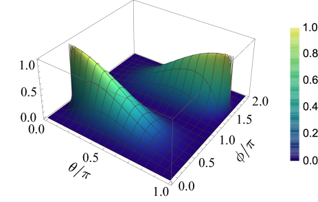
Figure 1: (Color online) $Q^{(\nicefrac{{1}}{{2}})}_{m}/Q_{0}$ as a function of $\theta$ and $\phi$.

Higher-dimensional pointer.—We consider $Q^{(j)}_{m}$ for $j\geq 1$. Detailed calculations are shown in the Supplementary Material Sub . We obtain $Q^{(j)}_{m}/Q^{(\nicefrac{{1}}{{2}})}_{m}\leq 2j$. The equality is satisfied when $(\phi,\theta)=(3\pi/2,0)$. In Fig. 2, $Q^{(j)}_{m}/Q^{(\nicefrac{{1}}{{2}})}_{m}$ is shown as a function of $\theta$ for $j=1,3/2,$ and 2. When $\phi=3\pi/2$ ($|(\sigma_{z})_{\rm m}|$ is maximum), $Q^{(j)}_{m}/Q^{(\nicefrac{{1}}{{2}})}_{m}$ can be larger than 1. On the other hand, its maximum is 1 when $\phi=\pi/2$ ($|(\sigma_{z})_{m}|$ is minimum). There is an advantage of the modular-value amplification in the case of $j\geq 1$.

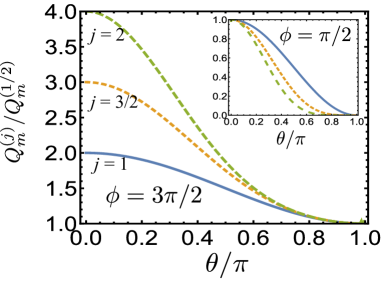
Figure 2: (Color online) $Q^{(j)}_{m}/Q^{(\nicefrac{{1}}{{2}})}_{m}$ for $j=1,3/2$ and 2 at $\phi=3\pi/2$ where $|(\sigma_{z})_{\rm m}|$ is maximum. Its maximum is $2j$ and can be achieved at $\theta=0$. Inset: the same as the main figure at $\phi=\pi/2$ where $|(\sigma_{z})_{\rm m}|$ is minimum.

Suppose that we have $L+1$ qubits as a resource for measurement. We may employ them as $L$ independent sensors and one qubit pointer. In this case, $\delta\omega$ scales $1/\sqrt{L}$ which corresponds to the standard quantum limit. In order to measure all sensors, we have to repeat measurements $L$ times. On the other hand, we can employ them as one qubit sensor and a $j\geq 1$ pointer formed with $L$ qubits. Note that $j=L/2$ Giraud114 . Therefore, we expect the enhancement of the Fisher information as $Q^{(j)}_{m}/Q^{(\nicefrac{{1}}{{2}})}_{m}=L$ according to the above discussion. If we are allowed to measure $L$ times as in the previous case, we may be able to expect another $L$ enhancement in the Fisher information. In total, the enhancement of the Fisher information can scale $L^{2}$. It implies $\delta\omega$ scales $1/{L}$. We claim that our modular-value-based measurement with a spin-$j$ coherent pointer can approach the Heisenberg limit.

Measurements under noise.—So far, we assumed the ideal noiseless environments. Let us consider measurements under noisy environments where phase-flip errors occur on the pointer. The influence of the noise is described by the operator-sum representation as Nielsen ; Desurvire ,

$$\rho^{\prime}=(1-\nu)\rho+\nu{\sigma}_{z}\rho{\sigma}_{z},$$ (8)

where $\rho^{\prime}$ is the density matrix of the pointer under the noise, $\rho$ is that in the noiseless environment, and $0<\nu<1$ is the probability of the phase-flip. When $\nu=1/2$, we totally lose the information of $\omega$ Desurvire . Hereafter, we only discuss a modular-value-based measurement with a qubit-pointer ($j=1/2$) as a concrete example of noisy measurements.

By using the symmetric logarithmic derivative (SLD) operators defined by $\hat{L}_{\lambda}\rho+\rho\hat{L}_{\lambda}=2\partial_{\lambda}\rho$ Braunstein72 ; Paris7 , the quantum Fisher information matrix $(H_{\alpha,\beta})$ is defined by Paris7 ; Fujiwara201 ; Matsumoto35 ; Helstrom25

$$H_{\alpha,\beta}=p(\omega){\rm Tr}\Bigl{[}\rho^{\prime}\dfrac{\hat{L}_{\alpha}\hat{L}_{\beta}+\hat{L}_{\beta}\hat{L}_{\alpha}}{2}\Bigr{]},$$ (9)

where $\alpha,\beta=\omega$ or $\nu$. $H_{\omega,\omega}$ is the quantum Fisher information associated with the estimation of $\omega$ and named as ${}^{\omega}Q^{(\nicefrac{{1}}{{2}})}_{m}$, while $H_{\nu,\nu}$ is that with the estimation of $\nu$ and named as ${}^{\nu}Q^{(\nicefrac{{1}}{{2}})}_{m}$. For $j=1/2$, the final density matrix of the pointer is given by $\rho=|\eta\rangle\langle\eta|$, where $|\eta\rangle$ is given by Eq. (6). Then, we obtain

$$H=\begin{pmatrix}\frac{(1-2\nu)^{2}t^{2}\sin^{2}\theta\sin^{2}\phi}{2(1-\sin\theta\sin\phi)}&0\\ 0&\frac{\sin^{2}\theta\cos^{2}\phi}{2(\nu-\nu^{2})(1-\cos\theta\sin\phi)}\end{pmatrix}+O(\omega^{2}).$$ (10)

We observe ${}^{\omega}Q^{(\nicefrac{{1}}{{2}})}_{m}=(1-2\nu)^{2}\ Q^{(\nicefrac{{1}}{{2}})}_{m}$: This fact clearly illustrates that the noise degrades the measurements and that the $\theta-$ and $\phi-$dependencies are inherited from $Q^{(\nicefrac{{1}}{{2}})}_{m}$ to ${}^{\omega}Q^{(\nicefrac{{1}}{{2}})}_{m}$. It is in agreement with the general discussion under noise Jordan2 , too.

We show $(\nu-\nu^{2})\ {}^{\nu}Q^{(\nicefrac{{1}}{{2}})}_{m}$ as a function of $\theta$ and $\phi$ in Fig. 3. It is interesting to note that ${}^{\nu}Q^{(\nicefrac{{1}}{{2}})}_{m}=0$ when $\phi=\pi/2$ and $3\pi/2$ and that these $\phi$’s give the maxima of ${}^{\omega}Q^{(\nicefrac{{1}}{{2}})}_{m}$. Even more interesting, the parameter combinations of $\theta=\pi/2$ and $\phi=n\pi$ ($n$: integer) give the maxima of ${}^{\nu}Q^{(\nicefrac{{1}}{{2}})}_{m}$ at the cost of ${}^{\omega}Q^{(\nicefrac{{1}}{{2}})}_{m}=0$. It implies that we can optimize the measurement of $\nu$, or noise, by selecting $\theta$ and $\phi$ properly. It is very important to measure noise since noise often causes relaxation of quantum systems.

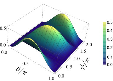
Figure 3: (Color online) $(\nu-\nu^{2})\ {}^{\nu}Q^{(\nicefrac{{1}}{{2}})}_{m}$ as a function of $\theta$ and $\phi$.

Conclusions.—We have investigated the modular-value-based measurements with spin-$j$ coherent pointers. We discussed two cases with $j=1/2$ and $j\geq 1$. From the viewpoint of quantum Fisher information, we first showed the modular-value-based measurements with a qubit pointer ($j=1/2$) has no merit in the sensitivity enhancement as in a weak-value-based measurement with a zero-mean Gaussian pointer. In contrast, the measurements with $j\geq 1$, the quantum Fisher information can become $2j$ times that of the qubit pointer. If $L$ qubits consist a spin coherent pointer, the Fisher information in one measurement scales as $L$. By taking into account the time required for measurements, we claimed that the total Fisher information scales as $L^{2}$ and thus we have a chance to approach the Heisenberg limit. Our study in the presence of phase-flip errors shows that we can optimize a measurement for detecting noise.

Acknowledgments.—This work was supported by CREST(JPMJCR1774), JST.

Supplementary Material for “Modular-value-based metrology with spin coherent pointers”

Appendix A Quantum Fisher information in the case of $j=1/2$: $Q_{m}^{(1/2)}$

We show the detailed calculation of the measured quantum Fisher information in the case of modular-value-based measurement with the spin-$j$ coherent state when $j=1/2$. Let remind us the final pointer state

$$|\eta\rangle=\dfrac{1}{\sqrt{2}}\Bigl{(}\cos\frac{\phi}{2}|\xi_{+}\rangle+\sin\frac{\phi}{2}e^{-i\omega t}|\xi_{-}\rangle\Bigr{)}/\sqrt{p(\omega)},$$ (1)

where,

$$|\xi_{\pm}\rangle=e^{-i\varphi}\sin\frac{\theta}{2}\Bigl{|}\frac{1}{2},-\frac{1}{2}\Bigr{\rangle}\mp i\cos\frac{\theta}{2}\Bigl{|}\frac{1}{2},+\frac{1}{2}\Bigr{\rangle},$$ (2)

$$p(\omega)=(1-\cos\theta\sin\phi\cos\omega t)/2,$$ (3)

$$\langle\xi_{\pm}|\xi_{\pm}\rangle=1,\ \langle\xi_{-}|\xi_{+}\rangle=\langle\xi_{+}|\xi_{-}\rangle=-\cos{\theta}.$$ (4)

Taking the derivative of the final pointer state, we obtain

$$\dfrac{d|\eta\rangle}{d\omega}=\dfrac{-it}{\sqrt{2p(\omega)}}\Bigl{(}\sin\frac{\phi}{2}e^{-i\omega t}|\xi_{-}\rangle\Bigr{)}.$$ (5)

Then, we have

$$\dfrac{d\langle\eta|}{d\omega}\dfrac{d|\eta\rangle}{d\omega} =\dfrac{t^{2}}{2p(\omega)}\sin^{2}\frac{\phi}{2},\ \text{and }$$ (6)

$$\dfrac{d\langle\eta|}{d\omega}|\eta\rangle =\dfrac{it}{2p(\omega)}\Bigl{[}\sin^{2}\frac{\phi}{2}-\frac{1}{2}\cos\theta\sin\phi e^{i\omega t}\Bigr{]}.$$ (7)

And thus, the measured quantum Fisher information yields

$$Q_{m}^{(\nicefrac{{1}}{{2}})} =4p(\omega)\Bigl{[}\dfrac{d\langle\eta|}{d\omega}\dfrac{d|\eta\rangle}{d\omega}-\Bigl{|}\dfrac{d\langle\eta|}{d\omega}|\eta\rangle\Bigr{|}^{2}\Bigr{]}$$

$$=\dfrac{t^{2}\sin^{2}\theta\sin^{2}\phi}{2(1-\cos\theta\sin\phi)}+O(\omega^{2}).$$ (8)

Equation (7) in the main text is obtained.

To calculate the postselected classical Fisher information $F_{p}$, we substitute

$$\dfrac{dp(\omega)}{d\omega}=\dfrac{t}{2}\cos\theta\sin\phi\sin\omega t$$ (9)

to Eq. (5), then we obtain $F_{p}=O(\omega^{2})$.

Appendix B Quantum Fisher information in the case of $j\geq 1$: $Q_{m}^{(j)}$

The final pointer state is the same as Eq. (1), where

$$|\xi_{\pm}\rangle =\exp\Bigl{(}\mp i\frac{\pi}{2}|j,+j\rangle\langle j,+j|\Bigr{)}|\xi\rangle$$

$$=\sum_{m=-j,j\geq 1}^{j-1}c_{jm}|j,m\rangle\mp i\Bigl{(}\cos\frac{\theta}{2}\Bigr{)}^{2j}|j,+j\rangle,$$ (10)

and

$$c_{jm}=\sqrt{{2j\choose j+m}}\Bigl{(}\cos\frac{\theta}{2}\Bigr{)}^{j+m}\Bigl{(}\sin\frac{\theta}{2}e^{-i\varphi}\Bigr{)}^{j-m},\ -j\leq m\leq j-1.$$ (11)

Then, we obtain

$$\langle\xi_{\pm}|\xi_{\pm}\rangle=1,\ \text{and }\langle\xi_{-}|\xi_{+}\rangle=\langle\xi_{+}|\xi_{-}\rangle=\sum_{m=-j}^{j-1}c_{m}^{2}-(\cos\frac{\theta}{2})^{4j},$$ (12)

as in the main text. Similar to the case of $j=1/2$, we calculate the derivative of the final pointer state as

$$\dfrac{d|\eta\rangle}{d\omega}=\dfrac{-it}{\sqrt{2p(\omega)}}\Bigl{(}\sin\frac{\phi}{2}e^{-i\omega t}|\xi_{-}\rangle\Bigr{)}.$$ (13)

Then, we have

$$\dfrac{d\langle\eta|}{d\omega}\dfrac{d|\eta\rangle}{d\omega}=\dfrac{t^{2}}{2p(\omega)}\sin^{2}\frac{\phi}{2},\ \text{and }\dfrac{d\langle\eta|}{d\omega}|\eta\rangle=\dfrac{it}{2p(\omega)}\Bigl{\{}\sin^{2}\frac{\phi}{2}+\frac{1}{2}\Bigl{[}\sum_{m=-j}^{j-1}c_{m}^{2}-(\cos\frac{\theta}{2})^{4j}\Bigr{]}\sin\phi e^{i\omega t}\Bigr{\}}.$$ (14)

The measured quantum Fisher information yields

$$Q_{m}^{(j)} =4p(\omega)\Bigl{[}\dfrac{d\langle\eta|}{d\omega}\dfrac{d|\eta\rangle}{d\omega}-\Bigl{|}\dfrac{d\langle\eta|}{d\omega}|\eta\rangle\Bigr{|}^{2}\Bigr{]}$$

$$=t^{2}\Biggl{\{}2\sin^{2}\dfrac{\phi}{2}-\dfrac{1}{p(\omega)}\Biggl{[}\sin^{2}\frac{\phi}{2}+\frac{1}{2}\Bigl{(}\sum_{m=-j}^{j-1}c_{m}^{2}-(\cos\frac{\theta}{2})^{4j}\Bigr{)}\sin\phi e^{i\omega t}\Biggr{]}^{2}\Biggr{\}}+O(\omega^{2}),$$ (15)

where

$$p(\omega)=\dfrac{1}{2}\Bigl{[}1+\Bigl{(}\sum_{m=-j}^{j-1}c_{m}^{2}-(\cos\frac{\theta}{2})^{4j}\Bigr{)}\cos\phi\cos\omega t\Bigr{]}.$$ (16)

From this result, we can easily calculate the measured quantum Fisher information for any given $j$.

References

- (1) C. L. Degen, F. Reinhard, and P. Cappellaro, Rev. Mod. Phys. 89, 035002 (2017).
- (2) Y. Matsuzaki, S. C. Benjamin, and J. Fitzsimons, Phys. Rev. A 84, 012103 (2011).
- (3) L. Pezzé and A. Smerzi, Phys. Rev. Lett. 102, 100401 (2009).
- (4) S. F. Huelga, C. Macchiavello, T. Pellizzari, A. K. Ekert, M. B. Plenio, and J. I. Cirac, Phys. Rev. Lett. 79, 3865 (1997).
- (5) W. M. Itano, J. C. Bergquist, J. J. Bollinger, J. M. Gilligan, D. J. Heinzen, F. L. Moore, M. G. Raizen, and D. J. Wineland, Phys. Rev. A 47, 3554 (1993).
- (6) M. Zwierz, C. A. Pérez-Delgado, and P. Kok, Phys. Rev. Lett. 105, 180402 (2010).
- (7) D. J. Wineland, J. J. Bollinger, W. M. Itano, F. L. Moore, and D. J. Heinzen, Phys. Rev. A 46, R6797 (1992).
- (8) D. J. Wineland, J. J. Bollinger, W. M. Itano, and D. J. Heinzen, Phys. Rev. A 50, 67 (1994).
- (9) V. Giovannetti, S. Lloyd, and L. Maccone, Science 306, 1330 (2004).
- (10) V. Giovannetti, S. Lloyd, and L. Maccone, Phys. Rev. Lett. 96, 010401 (2006).
- (11) J. A. Jones, S. D. Karlen, J. Fitzsimons, A. Ardavan, S. C. Benjamin, G. A. D. Briggs, and J. J. L. Morton, Science 324, 1166 (2009).
- (12) S. Simmons, J. A. Jones, S. D. Karlen, A. Ardavan, and J. J. L. Morton, Phys. Rev. A 82, 022330 (2010).
- (13) S. Zaiser, T. Rendler, I. Jakobi, T. Wolf, L. Sang-Yun, S. Wagner, V. Bergholm, T. Schulte-Herbrüggen, P. Neumann, and J. Wrachtrup, Nat. Comm. 7, 12279 (2016).
- (14) Y. Matsuzaki, S. Benjamin, S. Nakayama, S. Saito, and W. J. Munro, Phys. Rev. Lett. 120, 140501 (2018).
- (15) Y. Aharonov, D. Z. Albert, and L. Vaidman, Phys. Rev. Lett. 60, 1351 (1988).
- (16) Y. Aharonov and D. Rohrlich, Quantum Paradoxes: Quantum Theory for the Perplexed (Wiley-VCH, 2005).
- (17) A. G. Kofman, S. Ashhab, and F. Nori, Phys. Rep. 520, 43 (2012).
- (18) J. Dressel, M. Malik, F. M. Miatto, A. N. Jordan, and R. W. Boyd, Rev. Mod. Phys. 86, 307 (2014).
- (19) G. B. Alves, A. Pimentel, M. Hor-Meyll, S. P. Walborn, L. Davidovich, and R. L. deMatos Filho, Phys. Rev. A 95, 012104 (2017).
- (20) L. Zhang, A. Datta, and I. A. Walmsley, Phys. Rev. Lett. 114, 210801 (2015).
- (21) G. B. Alves, B. M. Escher, R. L. de Matos Filho, N. Zagury, and L. Davidovich, Phys. Rev. A 91, 062107 (2015).
- (22) S. Tanaka and N. Yamamoto, Phys. Rev. A 88, 042116 (2013).
- (23) G. C. Knee, G. A. D. Briggs, S. C. Benjamin, and E. M. Gauger, Phys. Rev. A 87, 012115 (2013).
- (24) G. C. Knee and E. M. Gauger, Phys. Rev. X 4, 011032 (2014).
- (25) S. Pang, J. Dressel, and T. A. Brun, Phys. Rev. Lett. 113, 030401 (2014).
- (26) S. Pang and T. A. Brun, Phys. Rev. A 92, 012120 (2015).
- (27) S. Pang and T. A. Brun, Phys. Rev. Lett. 115, 120401 (2015).
- (28) A. N. Jordan, J. Tollaksen, J. E. Troupe, J. Dressel, and Y. Aharonov, Quantum Studies: Mathematics and Foundations 2, 5 (2015).
- (29) Y. Kedem and L. Vaidman, Phys. Rev. Lett. 105, 230401 (2010).
- (30) L. B. Ho and N. Imoto, Phys. Lett. A 380, 2129 (2016).
- (31) L. B. Ho and N. Imoto, Phys. Rev. A 95, 032135 (2017).
- (32) L. B. Ho and N. Imoto, J. Math. Phys. 59, 042107 (2018).
- (33) L. B. Ho and N. Imoto, Phys. Rev. A 97, 012112 (2018).
- (34) J. P. Amiet and M. B. Cibils, J. Phys. A: Math. Gen. 24, 1515 (1991).
- (35) F. Bohnet-Waldraff, D. Braun, and O. Giraud, Phys. Rev. A 93, 012104 (2016).
- (36) C. R. Rao, Linear Statistical Inference and its Applications, 2nd ed. (Wiley, New York, 1973).
- (37) H. F. Hofmann, M. E. Goggin, M. P. Almeida, and M. Barbieri, Phys. Rev. A 86, 040102 (2012).
- (38) S. L. Braunstein and C. M. Caves, Phys. Rev. Lett. 72, 3439 (1994).
- (39) M. A. Nielsen and I. L. Chuang, Quantum Computation and Quantum Information, Cambridge University Press, (2000).
- (40) C. W. Helstrom, Quantum Detection and Estimation Theory (Academic Press, New York, 1976).
- (41) A. S. Holevo, Probabilistic and Statistical Aspects of Quantum Theory (North-Holland, Amsterdam, 1982).
- (42) J. Combes, C. Ferrie, Z. Jiang, and C. M. Caves, Phys. Rev. A 89, 052117 (2014).
- (43) See supplementary material for the detailed calculation of the measured quantum Fisher information.
- (44) O. Giraud, D. Braun, D. Baguette, T. Bastin, and J. Martin, Phys. Rev. Lett. 114, 080401 (2015).
- (45) E. Desurvire, Classical and Quantum Information Theory An Introduction for the Telecom Scientist, Cambridge University Press, (2009).
- (46) M. G. A. Paris, Int. J. Quantum Inf. 7, 125 (2009).
- (47) A. Fujiwara and H. Nagaoka, Phys. Lett. A 201, 119 (1995).
- (48) K. Matsumoto, J. Phys. A 35, 3111 (2002).
- (49) C. W. Helstrom, Phys. Lett. A 25, 101 (1967).