Minimal QCDF Model for $B\to\pi K$ Puzzle

Abstract

In this work, we propose a model by combining the parametrization method and the QCD factorization to study the $B\to\pi K$ puzzle. The parametrization for the $B\to\pi K$ amplitudes introduces twelve parameters, the weak angle $\gamma$ and the other eleven hadronic parameters. These hadronic parameters are assumed to be perturbative and can be calculated by the QCD factorization (QCDF). The calculational accuracy of the QCDF is improved by including the twist-3 three parton tree and one loop corrections. Three additional nonperturbative strong phases from the gluonic penguin, color suppressed, and color favored tree diagrams are required to account for the direct CP asymmetries. The weak angle, three nonperturbative strong phases, and four scale variables are assumed as fitting parameters. Four scale variables represent the factorization scales for the decays, each decay mode with one scale. These eight parameters are determined by a least squares fit to the eight measurements for $B\to\pi K$ decays, four branching ratios and four direct CP asymmetries. The fit shows that the hadronic parameters need to be process-dependent. A large negative relative phase associated with the internal up quark gluonic penguin diagram is observed. The weak angle $\gamma$ is found to be $72.1\pm 5.8$ degree, being consistent with the world averaged value, $72.1\pm 5.8$ degree. By a least squares fit to the mixing induced asymmetry $S(\pi^{0}K_{S})=0.58\pm 0.06$, the weak angle $\beta$ is determined to be $22.9\pm 2.1$ degree, which is in a well agreement with the world averaged value, $22.5\pm 4.4\pm 0.6$ degree. The model predicts the ratio $C^{\prime}/T^{\prime}$ (color suppressed/color favored) to be $0.59\pm 0.08$. The above evidences indicate that the model can solve the $B\to\pi K$ puzzle consistently. The model is used to examine the quadrangle relation of the isospin symmetry assumed for the $B\to\pi K$ system. The ratio of the two sides of the quadrangle relation is calculated to be $(0.87\pm 0.15)\exp(-i22^{\circ})$, which signals the isospin symmetry breaking at $6\sigma$. The process-dependent hadronic parameters break the isospin symmetry “dynamically”. The application of our method to other decay processes is straightforward.

PACS numbers

12.15.Ff,12.38.Bx,12.39.St,13.25.Hw, 14.40.Nd.

Keywords

perturbative QCD, factorization, isospin, B physics, CP violation, CKM mechanism.

I Introduction

In order to establish the CKM mechanism of the Standard Model (SM), the studies of hadronic $B$ decays have been devoted to construct the unitarity triangle $V_{ub}^{*}V_{ud}+V_{cb}^{*}V_{cd}+V_{tb}^{*}V_{td}=0$, for which a systematic procedure has been developed (Battaglia et al., 2003; Buras, 2005). Experimentally, many rare processes have been measured by BABAR, Belle and LHCb(Bevan et al., 2014). The benchmarks are the mixing induced CP asymmetry $S(B\to J/\psi K)=0.691\pm 0.017$ and the direct CP asymmetry $A_{CP}(B^{0}\to\pi^{-}K^{+})=-0.082\pm 0.006$ (Patrignani et al., 2016). However, there appeared many difficulties in theories. One of these is the $B\to\pi K$ puzzle:

1. The theoretical predictions for the branching ratios are smaller than the experimental data (Beneke et al., 2001; Keum et al., 2001; Li and Mishima, 2011; Bai et al., 2014).

2. The theoretical predictions for the CP asymmetries have a much different pattern from that of the experimental measurements (Li and Mishima, 2011; Beneke et al., 2001; Li et al., 2005; Keum et al., 2001; Bai et al., 2014; Khalil et al., 2009).

3. It is difficult to reach consistent explanations for different experimental measurements (Buras et al., 2004a, 2003, b).

At present, it seems still unable to solve the puzzle by model-independent methods (Neubert, 1999), such as the flavor symmetry approach (Buras et al., 2004a, 2003, b; Chiang et al., 2004; Fleischer et al., 2008), or the global-fit approach (Neubert, 1999; Chiang et al., 2004; Baek and London, 2007; Baek et al., 2009; Beaudry et al., 2018). The other possible method could be to employ the perturbative QCD (pQCD) theories (Beneke et al., 2001; Keum et al., 2001; Li and Mishima, 2011; Bai et al., 2014; Li and Mishima, 2011; Beneke et al., 2001; Li et al., 2005; Keum et al., 2001; Bai et al., 2014; Khalil et al., 2009). In this work, QCD factorization (QCDF)(Beneke et al., 1999; Beneke and Neubert, 2003; Beneke et al., 2001) is employed to provide a calculational framework. The concern will focus on how to disentangle the weak phases from the strong phases. Specifically, a model based on a general parametrization for the $B\to\pi K$ decay amplitudes will be constructed. There will introduce eleven hadronic parameters to be calculated by the QCDF. Three additional nonperturbative strong phases, which are closely related to the direct CP asymmetries, are required to explain the experimental data.

In addition, the model assumes that the parameters could be process-dependent. The reason is easy to understand from the point of view of the pQCD approach. Any parameter is expressed as a convolution integral of the short and long distance parts. Although the long distance part is process-independent, however, the process-dependence of the short distance part makes the hadronic parameter to be process-dependent. This means that the value of any parameter for different processes would be different. We will show that this point is important to find a solution to the puzzle.

In past years, the QCDF calculations have considered corrections up to twist-3 two parton and NNLO in $\alpha_{s}$ (Beneke et al., 2001; Bell, 2009; Beneke et al., 2010; Bell et al., 2015; Neubert and Pecjak, 2002). These calculations show no significant enhancements in the predictions for the branching ratios and direct CP asymmetries (Beneke et al., 2001). Since the $B\to\pi K$ decays are penguin dominated, there are twist-3 chirally enhanced corrections from the effective operator $Q_{6,8}$, for which there also exist three parton contributions. As indicated in Ref.(Yeh, 2008a), the tree level three parton terms could significantly improve the predictions for branching ratios. In order to improve the calculational accuracy, we will calculate the three parton contributions up-to one loop radiative corrections.

The organization is as follows. In Sec.II, a general parametrization method for the amplitudes (Imbeault et al., 2007; Buras and Silvestrini, 2000) will be used to construct the model for the $B\to\pi K$ decays. The model contains twelve parameters: the weak angle $\gamma$ and the other eleven parameters. An improved factorization formula up-to $O(\alpha_{s}^{2}/m_{b})$ will be constructed by including the three parton corrections. The formula will be used to calculate the parameters in SecIII. In SecIV, a fitting strategy will be developed to extract the weak and the strong phases from the data. According to the fitted result, the phenomenology analysis and discussions will be present in SecV. Conclusion will be given in SecVI.

II Model

II.1 Parameterizations

In general, the amplitudes for $B\to\pi K$ decays with $B=B^{\pm},B^{0}(\bar{B}^{0})$, $K=K^{\pm},K^{0}(\bar{K}^{0})$, and $\pi=\pi^{\pm},\,\pi^{0}$, could be parameterized as follows (Neubert, 1999; Buras and Silvestrini, 2000; Beneke et al., 2001; Gronau et al., 1999; Imbeault et al., 2007)

$$A(\pi^{-}\bar{K}^{0}) = P^{\prime}(1+\epsilon_{a}e^{i\phi_{a}}e^{-i\gamma})\,,$$ (1)

$$-\sqrt{2}A(\pi^{0}K^{-}) = P^{\prime}(1+\epsilon_{a}e^{i\phi_{a}}e^{-i\gamma}$$

$$-\epsilon_{3/2}e^{i\phi}(e^{-i\gamma}-qe^{i\omega}))\,,$$

$$-A(\pi^{+}K^{-}) = P^{\prime}(1+\epsilon_{a}e^{i\phi_{a}}e^{-i\gamma}$$

$$-\epsilon_{T}e^{i\phi_{T}}(e^{-i\gamma}-q_{C}e^{i\omega_{C}}))\,,$$

$$\sqrt{2}A(\pi^{0}\bar{K}^{0}) = P^{\prime}(1+\epsilon_{a}e^{i\phi_{a}}e^{-i\gamma}$$

$$+(\epsilon_{3/2}e^{i\phi}-\epsilon_{T}e^{i\phi_{T}})e^{-i\gamma}$$

$$+(\epsilon_{T}q_{C}e^{i(\phi_{T}+\omega_{C})}-\epsilon_{3/2}qe^{i(\phi+\omega)}))\,,$$

where $A(\pi K)$ mean the amplitudes of $B\to\pi K$ decays. In the above expressions, the “unitarity triangle” has been used to translate the contributions from $\lambda_{t}$ to the $\lambda_{u}$ and $\lambda_{c}$ terms, where $\lambda_{q}=V_{qb}^{*}V_{qd}$ for $q=u,\,c,\,t$. $P^{\prime}$ denotes the major penguin amplitude (containing $\lambda_{c}$). The weak angle $\gamma=arg(V_{ub}^{*})$ comes from the terms containing $\lambda_{u}$. The others are real parameters, $\epsilon_{a}$, $\epsilon_{3/2}$, $\epsilon_{T}$, $q$ and $q_{C}$ and their associated strong phases $\phi_{a},\,\phi,\,\phi_{T},\,\omega,\,\omega_{C}$ (Beneke et al., 2001). The amplitudes for $B^{+,0}$ are obtained by replacing the weak angle $\gamma$ by $-\gamma$. Some relative minor terms such as annihilation, exchange and penguin-annihilation terms have been neglected.

In Eqs.(1-II.1), the isospin symmetry is assumed. The initial $B$ meson $(B^{-},\,\bar{B}^{0})$ is of $I_{B}=-\frac{1}{2}$ state $|B(I=-\frac{1}{2})\rangle$. The final $(\pi K)$ state can be decomposed into the $I_{\pi K}=+\frac{1}{2}$ state $\langle\pi(I=1)K(I=-\frac{1}{2})|$, the $I_{\pi K}=-\frac{1}{2}$ state $\langle\pi(I=0)K(I=-\frac{1}{2})|$, and the $I=-\frac{3}{2}$ state $\langle\pi(I=-1)K(I=-\frac{1}{2})|$. The effective weak Hamiltonian has $\Delta I=0$ and $\Delta I=1$ operators, where $\Delta I\equiv|I_{B}-I_{\pi K}|$. Therefore, the matrix element $\langle\pi K|H_{eff}|B\rangle$ could be described by three isospin amplitudes $B_{1/2}$, $A_{1/2}$, and $A_{3/2}$, which correspond to $\Delta I=0$ with $I_{\pi K}=-\frac{1}{2}$, $\Delta I=1$ with $I_{\pi K}=+\frac{1}{2}$, $\Delta I=1$ with $I_{\pi K}=-\frac{3}{2}$, respectively. The decay amplitudes are expressed as (Neubert, 1999)

$$A(\pi^{-}\bar{K}^{0}) = B_{1/2}+A_{1/2}+A_{3/2}\,,$$ (5)

$$-\sqrt{2}A(\pi^{0}K^{-}) = B_{1/2}+A_{1/2}-2A_{3/2}\,,$$ (6)

$$-A(\pi^{+}K^{-}) = B_{1/2}-A_{1/2}-A_{3/2}\,,$$ (7)

$$\sqrt{2}A(\pi^{0}\bar{K}^{0}) = B_{1/2}-A_{1/2}+2A_{3/2}\,,$$ (8)

from which the quadrangle relation (Nir and Quinn, 1991; Gronau, 1991) is obtained

$$A(\pi^{-}\bar{K}^{0})+\sqrt{2}A(\pi^{0}K^{-})$$

$$= A(\pi^{+}K^{-})+\sqrt{2}A(\pi^{0}\bar{K}^{0})$$

$$= 3A_{3/2}\,.$$

These isospin amplitudes $B_{1/2},\,A_{1/2},\,A_{3/2}$ need to be process-independent. The same argument is applied to the eleven parameters, $P^{\prime}$, $\epsilon_{a}$, $\epsilon_{3/2}$, $\epsilon_{T}$, $q$, $q_{C}$, $\phi_{a},\,\phi,\,\phi_{T},\,\omega,\,\omega_{C}$. One should note that the isospin symmetry and the process-independence are closely correlated. It is interesting to examine whether the isospin symmetry could be preserved or broken, if the parameters are process-dependent. This will be made in latter text.

There are total twelve parameters to be determined, but we have only eight independent measurements, four sets of branching rates and asymmetries. (We identify the measurement for the mixing induced CP asymmetry $S_{\pi^{0}K_{S}^{0}}$ as an independent test for the weak angle $\beta$ and our model.) It is impossible to completely determine all the parameters. In the next section, the QCDF with three parton corrections is used to calculate the eleven hadronic parameters. Further more, the three phases $\phi_{a},\,\phi,\,\phi_{T}$ are assumed to contain both perturbative and nonperturbative QCD contributions. The perturbative parts $\hat{\phi}_{a},\,\hat{\phi},\,\hat{\phi}_{T}$, are calculated by the QCDF formalism. The nonperturbative $\bar{\phi}_{a},\,\bar{\phi},\,\bar{\phi}_{T}$ are determined by a least squares fit to the experimental data. We will also assume that the factorization scale $\mu$ for four processes are different, $\mu_{i}$, $i=1,\cdots,4$. Then, there are total eight parameters, $\bar{\phi}_{a},\,\bar{\phi},\,\bar{\phi}_{T}$, $\gamma$, and $\mu_{i}$, which can be completely determined by eight measurements. We identify this model as the minimal QCDF model (MQCDF).

II.2 Observables

In order to explicitly explore how the puzzle would happen, every term is remained in the following expressions without applying any approximation. Using the above parametrization for the amplitudes, the branching ratios are expressed as

$$Br(\pi^{-}K^{0}) = \Gamma_{B^{-}}P^{\prime 2}[1+2\epsilon_{a}\cos(\phi_{a})\cos(\gamma)+\epsilon_{a}^{2}]\,,$$ (10)

$$Br(\pi^{0}K^{-}) =\frac{1}{2}\Gamma_{B^{-}}P^{\prime 2}[1+\epsilon_{3/2}^{2}+\epsilon_{a}{}^{2}+\epsilon_{3/2}^{2}q^{2}$$ (11)

$$+2\epsilon_{a}\cos(\phi_{a})\cos(\gamma)-2\epsilon_{3/2}\text{cos}(\phi)\cos(\gamma)$$

$$+2\epsilon_{3/2}q\text{cos}(\omega+\phi)-2\epsilon_{3/2}\epsilon_{a}\text{cos}(\phi-\phi_{a})$$

$$-2\epsilon_{3/2}^{2}q\text{cos}(\omega)\cos(\gamma)$$

$$+2\epsilon_{3/2}\epsilon_{a}q\text{cos}(\omega+\phi-\phi_{a})\cos(\gamma)]\,,$$

$$Br(\pi^{+}K^{-}) =\Gamma_{B^{0}}P^{\prime 2}[1+\epsilon_{T}^{2}+\epsilon_{a}{}^{2}+\epsilon_{T}^{2}q^{2}$$ (12)

$$+2\epsilon_{a}\cos(\phi_{a})\cos(\gamma)-2\epsilon_{T}\text{cos}(\phi_{T})\cos(\gamma)$$

$$+2\epsilon_{T}q\text{cos}(\omega+\phi_{T})-2\epsilon_{T}\epsilon_{a}\text{cos}(\phi_{T}-\phi_{a})$$

$$-2\epsilon_{T}^{2}q\text{cos}(\omega)\cos(\gamma)$$

$$+2\epsilon_{T}\epsilon_{a}q\text{cos}(\omega+\phi_{T}-\phi_{a})\cos(\gamma)]\,,$$

$$Br(\pi^{0}K^{0}) =\frac{1}{2}\Gamma_{B^{0}}P^{\prime 2}[1+\epsilon_{a}{}^{2}+\epsilon_{3/2}^{2}$$ (13)

$$+\epsilon_{3/2}^{2}q^{2}+\epsilon_{T}^{2}+\epsilon_{T}^{2}q_{C}^{2}$$

$$+2\epsilon_{a}\cos(\phi_{a})\cos(\gamma)-2\epsilon_{3/2}\text{cos}(\phi)\cos(\gamma)$$

$$-2\epsilon_{T}\text{cos}(\phi_{T})\cos(\gamma)+2\epsilon_{3/2}q\text{cos}(\omega+\phi)$$

$$-2\epsilon_{3/2}\epsilon_{a}\text{cos}(\phi-\phi_{a})+2\epsilon_{T}q_{C}\text{cos}(\omega_{C}+\phi_{T})$$

$$-2\epsilon_{T}\epsilon_{a}\text{cos}(\phi_{T}-\phi_{a})-2\epsilon_{3/2}^{2}q\text{cos}(\omega)\cos(\gamma)$$

$$-2\epsilon_{T}^{2}q_{C}\text{cos}(\omega_{C})\cos(\gamma)$$

$$+2\epsilon_{3/2}\epsilon_{a}q\text{cos}(\omega+\phi-\phi_{a})\cos(\gamma)$$

$$+2\epsilon_{T}\epsilon_{a}q_{C}\text{cos}(\omega_{C}+\phi_{T}-\phi_{a})\cos(\gamma)]\,,$$

and the direct CP asymmetries written as

$$A_{CP}(\pi^{-}K^{0}) = N(\pi^{-}K^{0})\epsilon_{a}\sin(\phi_{a})\sin(\gamma)\,,$$ (14)

$$A_{CP}(\pi^{0}K^{-}) = N(\pi^{0}K^{-})\sin(\gamma)[\epsilon_{a}\sin(\phi_{a})$$

$$-\epsilon_{3/2}\sin(\phi)+\epsilon_{3/2}^{2}q\sin(\omega)$$

$$-\epsilon_{a}\epsilon_{3/2}q\sin(-\phi_{a}+\phi+\omega)]\,,$$

$$A_{CP}(\pi^{+}K^{-}) = N(\pi^{+}K^{-})\sin(\gamma)[\epsilon_{a}\sin(\phi_{a})$$

$$-\epsilon_{T}\sin(\phi_{T})+\epsilon_{T}^{2}q_{C}\sin(\omega_{C})$$

$$-\epsilon_{a}\epsilon_{T}q\sin(-\phi_{a}+\phi_{T}+\omega_{C})]\,,$$

$$A_{CP}(\pi^{0}K^{0}) = N(\pi^{0}K^{0})\sin(\gamma)[\epsilon_{a}\sin(\phi_{a})$$

$$+(\epsilon_{3/2}\sin(\phi)-\epsilon_{T}\sin(\phi_{T}))$$

$$+(\epsilon_{3/2}^{2}q\sin(\omega)+\epsilon_{T}^{2}q_{C}\sin(\omega_{C}))$$

$$+\epsilon_{a}(\epsilon_{3/2}q\sin(-\phi_{a}+\phi+\omega)$$

$$-\epsilon_{T}q_{C}\sin(-\phi_{a}+\phi_{T}+\omega_{C}))$$

$$-\epsilon_{3/2}(\epsilon_{T}q\sin(\phi-\phi_{T}+\omega)$$

$$+\epsilon_{T}q_{C}\sin(-\phi+\phi_{T}+\omega_{C}))]\,,$$

where

$$N(\pi K) = \frac{2P^{{}^{\prime}2}\Gamma_{B}}{Br(\pi K)}\,.$$

The branching ratios are calculated according to

$$Br(B\to\pi K) = \frac{1}{2}\Gamma_{B}(\left|A(B\to\pi K)\right|^{2}+\left|A(\bar{B}\to\pi K)\right|^{2})$$

where

$$\Gamma_{B} = \frac{\tau_{B}}{16\pi m_{B}}\,.$$

According to the particle data group (PDG) definition (Patrignani et al., 2016), the CP asymmetry is defined by

$$A_{CP} = \frac{Br(\bar{B}\to\bar{f})-Br(B\to f)}{Br(\bar{B}\to\bar{f})+Br(B\to f)}\,.$$

Three ratios

$$R = \frac{Br(\pi^{+}K^{-})+Br(\pi^{0}K^{0})}{Br(\pi^{-}K^{0})+Br(\pi^{0}K^{-})}\frac{\Gamma_{B^{-}}}{\Gamma_{B^{0}}}\,,$$ (18)

$$R_{c} = 2\left[\frac{Br(B^{-}\to\pi^{0}K^{-})}{Br(B^{-}\to\pi^{-}\bar{K}^{0})}\right]\,,$$ (19)

$$R_{n} = \frac{1}{2}\left[\frac{Br(\bar{B}^{0}\to\pi^{-}K^{+})}{Br(\bar{B}^{0}\to\pi^{0}K^{0})}\right]\,,$$ (20)

have been widely used in literature as tests for the SM. The comparisons between the theoretical predictions and experimental data of these quantities are left to Sec.V.

III Calculations

At the factorization scale $\mu\sim m_{b}$ (the bottom quark mass), the effective weak Hamiltonian for $B\to\pi K$ decays is given by (Buchalla et al., 1996; Buras, 1998)

$$H_{eff} = \frac{G_{F}}{\sqrt{2}}\sum_{p=u,c}\lambda_{p}\left[C_{1}(\mu)Q_{1}^{p}(\mu)+C_{2}(\mu)Q_{2}^{p}(\mu)\right.$$

$$+\sum_{i=3,\cdots,10}C_{i}(\mu)Q_{i}(\mu)+C_{7\gamma}(\mu)Q_{7\gamma}(\mu)$$

$$\left.+C_{8G}(\mu)Q_{8G}(\mu)\right]+h.c.$$

where $\lambda_{p}=V_{ps}^{*}V_{pb}$ is the product of CKM matrix elements. The local $\Delta B=1$ four quark operators $Q_{i}$ are defined as

$$Q_{1}^{p} = (\bar{s}_{\alpha}p_{\alpha})_{(V-A)}(\bar{p}_{\beta}b_{\beta})_{(V-A)}\,,$$ (22)

$$Q_{2}^{p} = (\bar{s}_{\alpha}p_{\beta})_{(V-A)}(\bar{p}_{\beta}b_{\alpha})_{(V-A)}\,,$$

$$Q_{3,5} = (\bar{s}_{\beta}b_{\beta})_{(V-A)}\sum_{q^{\prime}}(\bar{q}_{\alpha}^{\prime}q_{\alpha}^{\prime})_{(V\mp A)}\,,$$

$$Q_{4,6} = (\bar{s}_{\beta}b_{\alpha})_{(V-A)}\sum_{q^{\prime}}(\bar{q}_{\alpha}^{\prime}q_{\beta}^{\prime})_{(V\mp A)}\,,$$

$$Q_{7,9} = \frac{3}{2}(\bar{s}_{\beta}b_{\beta})_{(V-A)}\sum_{q^{\prime}}e_{q^{\prime}}(\bar{q}_{\alpha}^{\prime}q_{\alpha}^{\prime})_{(V\pm A)}\,,$$

$$Q_{8,10} = \frac{3}{2}(\bar{s}_{\beta}b_{\alpha})_{(V-A)}\sum_{q^{\prime}}e_{q^{\prime}}(\bar{q}_{\alpha}^{\prime}q_{\beta}^{\prime})_{(V\mp A)}\,,$$

$$Q_{7\gamma} = -\frac{e}{8\pi^{2}}(\bar{q}\sigma^{\mu\nu}(1+\gamma_{5})b)F_{\mu\nu}\,,$$

$$Q_{8G} = -\frac{g}{8\pi^{2}}m_{b}(\bar{q}\sigma^{\mu\nu}(1+\gamma_{5})b)G_{\mu\nu}\,,$$

where $q^{\prime}\in\left\{u,d,s,c,b\right\}$, $\alpha$ and $\beta$ mean color indices, and $e_{q^{\prime}}=2/3(-1/3)$ for $u(d)$ type quarks. The Wilson coefficients $C_{i}(\mu)$ collect the radiative contributions between $\mu$ and $M_{W}$ up to next-to-leading order (NLO) in $\alpha_{s}$. The renormalization scheme is chosen as the minimal-subtraction ($\overline{MS}$) with $\Lambda_{\overline{MS}}^{(5)}=0.225$ GeV. The $C_{i}$ are calculated by the naive dimensional regularization (NDR).

Assume the naive factorization $\langle\pi K|Q_{i}(0)|B\rangle=\langle\pi|\bar{q}_{1}\Gamma_{i,\mu}b|B\rangle\langle K|\bar{q}_{2}\Gamma_{i}^{\mu}q_{3}|0\rangle$ or $\langle K|\bar{q}_{1}\Gamma_{i,\mu}b|B\rangle\langle\pi|\bar{q}_{2}\Gamma_{i}^{\mu}q_{3}|0\rangle$, with $\Gamma_{u,i}\otimes\Gamma_{i}^{\mu}=\gamma_{\mu}(1-\gamma_{5})\otimes\gamma^{\mu}(1\pm\gamma_{5})$, and include possible one loop radiative corrections to the factorized terms, the hadronic matrix element $\langle\pi K|Q_{i}(0)|B\rangle$ could be expressed in the following factorized form, up-to the twist-3 and NLO in $\alpha_{s}$,

$$\langle\pi K|Q_{i}(0)|B\rangle$$

$$= F_{0}^{B\pi}(0)\int_{0}^{1}du\text{Tr}[T_{i,K}^{I}(u)\phi^{K}(u)]$$

$$+F_{0}^{BK}(0)\int_{0}^{1}du\text{Tr}[T_{i,\pi}^{I}(u)\phi^{\pi}(u)]$$

$$+\int_{0}^{\infty}d\xi\int_{0}^{1}du\int_{0}^{1}dv\text{Tr}[\phi^{B}(\xi)T_{i,B\pi K}^{II}(\xi,\,u,\,v)$$

$$\phi^{\pi}(u)\phi^{K}(v)]$$

where Tr means the trace taken over the spin indices and the integrals are made over the momentum fractions $u,\,v$, $\xi$. The hard scattering kernels, $T^{I,II}$, describe the short distance interactions between partons of the external initial and final state mesons. The kernel $T^{I}$ contains tree (T), vertex (V), and penguin (P) contributions. The kernel $T^{II}$ contains hard spectator (HS). The transition form factors, $F_{0}^{B\pi}$ and $F_{0}^{BK}$, and the meson spin distribution amplitudes $\phi^{B}$, $\phi^{\pi}$, $\phi^{K}$ encode the long distance interactions of the quarks and gluons. The validity of the factorization formula is explained below.

The factorization at leading twist order has been well-known (Beneke et al., 2001; Beneke and Neubert, 2003). In the following, let’s concentrate on the twist-3 level.

At the twist-3 two parton order, the hard spectator terms may contain end-point divergences in the form

$$X_{H} = \int_{0}^{1}du\frac{\phi_{p}(u)}{u}\,,$$ (24)

if the twist-3 two parton pseudo-scalar distribution amplitude $\phi_{p}$ is a constant (Beneke and Neubert, 2003; Beneke et al., 2001). This viewpoint of a constant $\phi_{p}$ has been widely employed in literature. However, this is not the correct fact, because a constant $\phi_{p}$ is determined by the equation of motion (EOM) at the chiral symmetry breaking scale $\mu_{c}\sim 1$ GeV. The partons involving in the hard scattering kernels $T^{II}$ would have energies about the energetic scale $\mu_{E}\sim m_{b}\gg\mu_{c}$. The correct EOM of $\phi_{p}$ would be taken at the energetic scale $\mu_{E}$ instead of $\mu_{c}$. As a result, $\phi_{p}$ becomes equal to $\phi_{\sigma}$ and not a constant. The above mentioned end-point divergences in the hard spectator terms would vanish (Yeh, 2008a).

There also exist end-point divergences from the annihilation terms in the form

$$X_{A} = \int_{0}^{1}du\frac{\phi_{P}(u)}{u(u-\xi)}\,,$$ (25)

even for the twist-2 pseudo-scalar distribution amplitude $\phi_{P}$ (Beneke et al., 2001; Beneke and Neubert, 2003). The regularization method is not to neglect the momentum fraction factor $\xi$ from the spectator lines of the $B$ meson. It can be shown that the regularized result is equivalent to include the twist-4 contributions (Yeh, 2008b). As a result, the annihilation terms up to twist-3 are also factorizable. The annihilation terms are not included in the above factorization formula and will be neglected in later calculations.

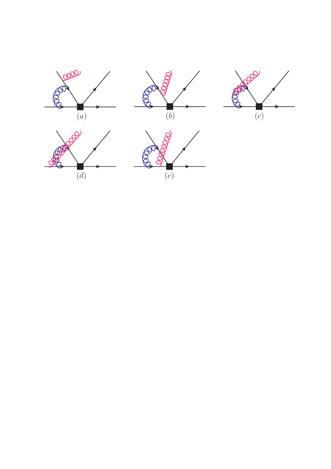
Figure 1: Three parton one loop diagrams for the vertex corrections of $T^{I}$ are shown. The red gluon line means the gluonic parton $g$ of the three parton $|q\bar{q}g\rangle$ state of the external $M_{2}$ meson state $|M_{2}\rangle$. The blue gluon line means the radiative loop gluons. The black box means the effective four quark operator. The other similar diagrams with the gluonic parton line connected to other external or internal parton lines to the vertex or penguin radiative loop corrections may also contribute. Similar three parton one loop diagrams for the $T^{II}$ are not shown here. The figure refers to (Yeh, 2008b).

According to the study by Yeh (Yeh, 2008b), there are five types of different ways as shown in Fig.1 that the three parton state $|q\bar{q}g\rangle$ of the emitted final state meson $M=\pi,\,K$ can contribute at one loop level. The three parton state from the $B$ meson needs not be considered, because only soft spectator gluonic partons can involve and their contributions are power suppressed by $O(1/m_{B}^{2})$. By power counting (Yeh, 2008a), it is easy to see that only contributions from Fig. 1(a) are leading at twist-3 order (i.e., suppressed by $O(1/m_{B})$) and the other types of contributions are at least of twist-4 (i.e., suppressed by $O(1/m_{B}^{2})$ than the leading twist-2 term). Considering only contributions from Fig.1(a), the meson spin distribution amplitude $\phi^{M}(u)$ for $M=\pi,\,K$ has the following spin representation (Yeh, 2008a)

$$\phi^{M}(u)$$ (26)

$$= \int_{0}^{\infty}\frac{d\lambda}{2\pi}e^{-iu\lambda}\langle M|\bar{q}_{a}(0)q_{b}(\frac{\lambda}{E}n)|0\rangle$$

$$+\int_{0}^{\infty}\frac{d\lambda}{2\pi}\int_{0}^{\infty}\frac{d\eta}{2\pi}e^{-i\alpha\lambda}e^{-i\beta\eta}\langle M_{2}|\bar{q}_{a}(0)ig\not\!A(\frac{\eta}{E}n)q_{b}(\frac{\lambda}{E}n)|0\rangle$$

$$= -\frac{if_{M}}{4N_{c}}\left[\gamma_{5}\not q\phi_{P}(u)+\mu_{\chi}\left(\gamma_{5}\phi_{p}(u)-\frac{1}{2}\epsilon_{\perp}\cdot\sigma\phi_{\sigma}(u)\right.\right.$$

$$\left.\left.+2\gamma_{5}\delta(u-\alpha-\beta)\int_{0}^{1}d\alpha\int_{0}^{(1-\alpha)}d\beta\frac{\phi_{3p}(\alpha,\beta)}{\alpha\beta}\right)\right]$$

where $\epsilon_{\perp}\cdot\sigma=\epsilon_{\alpha\beta\eta\lambda}\sigma^{\alpha\beta}\bar{n}^{\gamma}n^{\lambda}$ with $\bar{n}^{\mu}$ and $n^{\mu}$ being light like unit vector satisfying $\bar{n}^{2}=n^{2}=0$ and $\bar{n}\cdot n=1$. $f_{M}$ is the decay constant and $\mu_{\chi}^{M}=m_{M}^{2}/(m_{q_{a}}+m_{q_{b}})$ is the chiral enhanced factor. $\phi_{P}$ is the twist-2 pseudo-scalar distribution function and $\phi_{p}$ and $\phi_{\sigma}$ are twist-3 two parton pseudo-scalar and pseudo-tensor distribution functions. The three parton distribution function $\phi_{3p}$ is defined by

$$\int_{0}^{\infty}\frac{d\lambda}{2\pi}\int_{0}^{\infty}\frac{d\eta}{2\pi}e^{-i\alpha\lambda}e^{-i\beta\eta}$$ (27)

$$\langle M_{2}|\bar{q}(0)\gamma_{5}\sigma^{\alpha\beta}gG^{\mu\nu}(\frac{\eta}{E}n)q(\frac{\lambda}{E}n)|0\rangle$$

$$= -if_{M_{2}}\mu_{\chi}P^{\alpha\beta\mu\nu}(q)\phi_{3p}(\alpha,\beta)$$

and has a parametrization

$$\phi_{3p}(\alpha,\beta) = 360\eta\alpha\beta^{2}(1-\alpha-\beta)(1+\frac{1}{2}\omega(7\beta-3))$$ (28)

with $\eta=0.015$ and $\omega=-3$. This representation of the spin distribution $\phi^{M}$ is written according to the following facts:

• The effective spin structure and the integrals of $\phi_{3p}$ can be derived from the tree level Feynman diagrams similar to Fig.1(a), in which the radiative gluon is absorbed by the vertex. The detailed derivations refer to (Yeh, 2008a). When the three parton one loop Feynman diagrams as depicted in Fig.1(a) are considered, it can be easily derived that the same spin structure is also applicable. Effectively, one may regard the three parton in this scenario as a pseudo-scalar two parton term. This shows a very convenient way to calculate the three parton one loop corrections by referring to those one loop calculations of $\phi_{p}$ (Yeh, 2008b).

• It can be shown that the energetic EOM $\phi_{p}=\phi_{\sigma}$ (Yeh, 2008a) would not change if $\phi_{3p}$ is considered. This is because the spin projector $P^{\alpha\beta\mu\nu}(q)$ vanishes at the energetic EOM condition. It implies that $\phi_{p}$ and $\phi_{\sigma}$ decouple from $\phi_{3p}$ at the energetic limit $E\gg\Lambda_{QCD}$.

Combining the above two facts, it can be shown that the one loop corrections of $\phi_{3p}$ are factorizable according to the analysis for the factorizability of the one loop corrections of $\phi_{p}$ given in (Yeh, 2008b). The complete analysis of the above arguments will be present elsewhere. The $B$ meson spin distribution amplitude is given by (Yeh, 2008b)

$$\phi^{B}(\xi) =\int_{0}^{\infty}\frac{d\lambda}{2\pi}e^{-i\xi\lambda}\langle 0|\bar{q}(0)b(\frac{\lambda}{E}n)|B\rangle$$

$$=\frac{if_{B}}{4N_{c}}\left[(\not P_{B}+m_{B})\gamma_{5}\phi_{B}(\xi)\right]\,.$$

For numeric calculations, we employ the following models

$$\phi_{P}(u) = \phi_{p}(u)=6u(1-u)\,,$$ (30)

$$\phi_{B}(\xi) = \frac{N_{B}\xi^{2}\bar{\xi}^{2}}{[\xi^{2}+\epsilon_{B}\bar{\xi}]^{2}}\,,$$ (31)

with $N_{B}=0.133$, $\epsilon_{B}=0.005$ for $\lambda_{B}=350\;\text{MeV}$. $N_{B}$ and $\epsilon_{B}$ are determined by the moments

$$\int_{0}^{1}d\xi\phi_{B}(\xi) = 1,\;\int_{0}^{1}d\xi\frac{\phi_{B}(\xi)}{\xi}=\frac{m_{B}}{\lambda_{B}}\,,$$ (32)

where the errors are controlled within $1\%$. Since the radiative corrections for the meson distribution amplitudes start at NNLO $O(\alpha_{s}^{2})$, they could be neglected at NLO calculations.

Summarizing the above analysis, it shows that the factorization formula of QCDF given in Eq.(III) is valid up-to complete twist-3 power corrections and NLO in $\alpha_{s}$. Due to their smallness as compared with the other types of contributions, we will completely neglect the annihilation terms. This makes our later explanations for the puzzle completely different from most literature based on QCDF, in which the annihilation electro-weak penguin terms would be important (Beneke et al., 2001; Beneke and Neubert, 2003).

In the following, the tree, vertex, penguin, and hard spectator contributions are collected as $a^{p}_{i}(\pi K)$ for each $Q_{i}$ as given below

$$a_{i}^{p}(\pi K,\mu)$$

$$= (C_{i}(\mu)+\frac{C_{i\pm 1}(\mu)}{N_{c}})N_{i}(K)$$

$$+ \frac{C_{i\pm 1}(\mu)}{N_{c}}\frac{\alpha_{s}(\mu)C_{F}}{4\pi}\left[V_{i}^{(2)}(K)+V_{i}^{(3)}(K)\right]$$

$$+ (4\pi\alpha_{s}(\mu)C_{F})\frac{C_{i\pm 1}(\mu)}{N_{c}^{2}}\left[H_{i}^{(2)}(\pi K)+H_{i}^{(3)}(\pi K)\right]$$

$$+ P_{i}^{p(2)}(K,\mu)+P_{i}^{p(3)}(K,\mu)\,.$$

The expressions for the tree $N_{i}(K)$, the two parton vertex $V_{i}^{(2)}(K)$, the two parton hard spectator $H_{i}^{(2)}(\pi K)$, and the two parton penguin $P_{i}^{p(2)}(K)$ are referred to (Yeh, 2008b; Beneke et al., 2001). Here, we only present the three parton vertex $V_{6,8}^{(3)}(K)$, the three parton hard spectator $H_{i}^{(3)}(\pi K)$, and the three parton penguin $P_{6,8}^{p(3)}(K,\mu)$ as follows

$$V_{6,8}^{(3)}(K)$$ (34)

$$= 2\int_{0}^{1}d\alpha\int_{0}^{(1-\alpha)}d\beta {\displaystyle\left[\frac{\phi_{3p}(\alpha,\beta)(-6+h^{(3)}(\alpha,\beta))}{\alpha\beta}\right]}\,,$$

where the kernel is

$$h^{(3)}(\alpha,\beta) = 2\left[\text{Li}_{2}(x)+\frac{1}{2}(\ln\bar{x})^{2}-(x\leftrightarrow(1-x))\right]_{x=\alpha+\beta}\,.$$ (35)

The penguin functions $P_{6,8}^{p(3)}(K,\,\mu)$ are given by

$$P_{6}^{p(3)}(K,\mu)$$

$$= \frac{\alpha_{s}(\mu)C_{F}}{4\pi N_{c}}\left\{C_{1}(\mu)\left[\left(\frac{4}{3}\ln\frac{m_{b}}{\mu}+\frac{2}{3}\right)A_{G}-G_{K}^{(3)}(s_{p})\right]\right.$$

$$+C_{3}(\mu)\left[2\left(\frac{4}{3}\ln\frac{m_{b}}{\mu}+\frac{2}{3}\right)A_{G}-G_{K}^{(3)}(0)-G_{K}^{(3)}(1)\right]$$

$$+(C_{4}(\mu)+C_{6}(\mu))\left[\frac{4}{3}n_{f}\left(\ln\frac{m_{b}}{\mu}\right)A_{G}\right.$$

$$\left.-(n_{f}-2)G_{K}^{(3)}(0)-G_{K}^{(3)}(s_{c})-G_{K}^{(3)}(1)\right]$$

$$\left.-4C_{8g}^{\text{eff}}\int_{0}^{1}d\alpha\int_{0}^{(1-\alpha)}d\beta\frac{\phi_{3p}(\alpha,\beta)}{\alpha\beta}\right\}\,,$$

$$P_{8}^{p(3)}(\mu)$$

$$= \frac{\alpha}{9\pi N_{c}}\left\{(C_{1}(\mu)+N_{c}C_{2}(\mu))\right.$$

$$\left[\frac{4}{3}A_{G}\ln\frac{m_{b}}{\mu}+\frac{2}{3}A_{G}-G_{K}^{(3)}(s_{p})\right]$$

$$\left.-6C_{7\gamma}^{\text{eff}}\int_{0}^{1}d\alpha\int_{0}^{(1-\alpha)}d\beta\frac{\phi_{3p}(\alpha,\beta)}{\alpha\beta}\right\}\,,$$

where $n_{f}=5$ denotes the number of the flavors.

The functions $G_{K}^{(3)}(s_{p})$ is defined as

$$\hat{G}_{K}^{(3)}(s_{p}) = 2\int_{0}^{1}d\alpha\int_{0}^{(1-\alpha)}d\beta\frac{\phi_{3p}(\alpha,\beta)}{\alpha\beta}G(s-i\epsilon,1-x)|_{x=\alpha+\beta}\,,$$

$$G(s,u) = -4\int_{0}^{1}dxx(1-x)\ln[s-x(1-x)u]\,.$$

By substituting $s_{p}=0,\,m_{c}^{2}/m_{b}^{2},\,1$, $\hat{G}_{K}^{(3)}(s_{p})$ are calculated for later numerical analysis

$$\hat{G}_{K}^{(3)}(0) = 0.81-i1.23\,,$$

$$\hat{G}_{K}^{(3)}(s_{c}) = 1.26-i0.94\,,$$

$$\hat{G}_{K}^{(3)}(1) = 0.059\,.$$

The effective Wilson coefficients $C_{7\gamma}^{\text{eff}}$ and $C_{8g}^{\text{eff}}$ are calculated at their leading order in $\alpha_{s}$ to be constants

$$C_{7\gamma}^{\text{eff}} = -0.32\,,$$ (38)

$$C_{8g}^{\text{eff}} = -0.15\,.$$ (39)

The hard spectator functions $H_{i}^{(3)}(\pi K)$ are, for $i=1-5,\,7,\,9,\,10$,

$$H_{i}^{(3)}(\pi K)$$

$$= 2\frac{B_{\pi K}}{A_{\pi K}}m_{B}r_{\chi}^{\pi}(\mu_{h})\int_{0}^{1}d\xi\frac{\phi_{B}(\xi)}{\xi}\int_{0}^{1}d\alpha\int_{0}^{(1-\alpha)}d\beta\int_{0}^{1}du$$

$$\times \left[\frac{\phi_{3p}(\alpha,\beta)\phi_{P}(u)}{(\alpha+\beta)\alpha\beta(\bar{u}-\xi)}\right]\,,$$

where

$$B_{\pi K} = i\frac{G_{F}}{\sqrt{2}}f_{B}f_{K}f_{\pi}$$ (41)

and $H_{6,8}^{(2,3)}(\pi K)=0$. The scale in $r_{\chi}^{\pi}(\mu_{h})$ is assumed as $\mu_{h}=\sqrt{\Lambda_{h}\mu}$ and $\Lambda_{h}=0.5\;\text{GeV}$.

According to the QCD factorization formula Eq.(1), we obtain the expressions for the amplitudes (Beneke and Neubert, 2003; Beneke et al., 2001; Yeh, 2008b)

$$A(\pi^{-}\bar{K}^{0}) =\lambda_{p}A_{\pi K}\left[\left(a_{4}^{p}-\frac{1}{2}a_{10}^{p}\right)\right.$$ (42)

$$\left.+r_{\chi}^{K}\left(a_{6}^{p}-\frac{1}{2}a_{8}^{p}\right)\right]\,,$$

$$-\sqrt{2}A(\pi^{0}K^{-}) =A_{\pi K}\left[\lambda_{u}a_{1}+\lambda_{p}\left(a_{4}^{p}+a_{10}^{p}\right)\right.$$ (43)

$$\left.+\lambda_{p}r_{\chi}^{K}\left(a_{6}^{p}+a_{8}^{p}\right)\right]$$

$$+A_{K\pi}\left[\lambda_{u}a_{2}+\lambda_{p}\frac{3}{2}\left(-a_{7}+a_{9}\right)\right]\,,$$

$$-A(\pi^{+}K^{-}) =A_{\pi K}\left[\lambda_{u}a_{1}+\lambda_{p}\left(a_{4}^{p}+a_{10}^{p}\right)\right.$$ (44)

$$\left.+\lambda_{p}r_{\chi}^{K}\left(a_{6}^{p}+a_{8}^{p}\right)\right]\,,$$

$$\sqrt{2}A(\pi^{0}\bar{K}^{0}) =\lambda_{p}A_{\pi K}\left[\left(a_{4}^{p}-\frac{1}{2}a_{10}^{p}\right)\right.$$ (45)

$$\left.+r_{\chi}^{K}\left(a_{6}^{p}-\frac{1}{2}a_{8}^{p}\right)\right]$$

$$-A_{K\pi}\left[\lambda_{u}a_{2}+\lambda_{p}\frac{3}{2}\left(-a_{7}+a_{9}\right)\right]\,,$$

where the $\mu$ dependence of $a_{i}$ is implicitly understood. We have defined the following factors

$$A_{\pi K} = i\frac{G_{F}}{\sqrt{2}}(m_{B}^{2}-m_{\pi}^{2})F_{0}^{B\pi}(m_{K}^{2})f_{K}\,,$$ (46)

$$A_{K\pi} = i\frac{G_{F}}{\sqrt{2}}(m_{B}^{2}-m_{K}^{2})F_{0}^{BK}(m_{\pi}^{2})f_{\pi}\,,$$ (47)

$$r_{\chi}^{K} = \frac{2m_{K}^{2}}{m_{b}(m_{q}+m_{s})}(1+A_{G})\,,$$ (48)

$$\lambda_{u} = \lambda_{c}\tan^{2}\theta_{c}R_{b}e^{-i\gamma}\,,$$ (49)

$$\tan^{2}\theta_{c} = \frac{\lambda^{2}}{1-\lambda^{2}}\,,$$ (50)

$$R_{b} = \frac{1-\lambda^{2}/2}{\lambda}\left|\frac{V_{ub}}{V_{cb}}\right|\,,$$ (51)

$$\lambda = |V_{us}|\,.$$ (52)

The three parton tree factor $A_{G}$ comes from the integration (Yeh, 2008a)

$$A_{G} = 2\int_{0}^{1}d\alpha\int_{0}^{(1-\alpha)}d\beta\frac{\phi_{3p}(\alpha,\beta)}{\alpha\beta}\,.$$ (53)

By comparing expressions given in Eqs.(1-II.1) and Eqs.(42-45), the perturbative parts of the amplitude parameters are calculated to be (Beneke and Neubert, 2003)

$$P^{\prime} = \lambda_{c}A_{\pi K}\left[\left(a_{4}^{c}-\frac{1}{2}a_{10}^{c}\right)+r_{\chi}^{K}\left(a_{6}^{c}-\frac{1}{2}a_{8}^{c}\right)\right]\,,$$ (54)

$$\epsilon_{a}e^{i\hat{\phi}_{a}} = \epsilon_{KM}\frac{\left(a_{4}^{u}-\frac{1}{2}a_{10}^{u}\right)+r_{\chi}^{K}\left(a_{6}^{u}-\frac{1}{2}a_{8}^{u}\right)}{\left(a_{4}^{c}-\frac{1}{2}a_{10}^{c}\right)+r_{\chi}^{K}\left(a_{6}^{c}-\frac{1}{2}a_{8}^{c}\right)}\,,$$ (55)

$$\epsilon_{3/2}e^{i\hat{\phi}} = -\epsilon_{KM}$$

$$\times \frac{a_{1}+R_{\pi K}a_{2}+\frac{3}{2}\left(a_{10}^{u}+r_{\chi}^{K}a_{8}^{u}+R_{\pi K}\left(a_{9}-a_{7}\right)\right)}{\left(a_{4}^{c}-\frac{1}{2}a_{10}^{c}\right)+r_{\chi}^{K}\left(a_{6}^{c}-\frac{1}{2}a_{8}^{c}\right)}\,,$$

$$\epsilon_{T}e^{i\hat{\phi}_{T}} = -\epsilon_{KM}\frac{a_{1}+\frac{3}{2}\left(a_{10}^{u}+r_{\chi}^{K}a_{8}^{u}\right)}{\left(a_{4}^{c}-\frac{1}{2}a_{10}^{c}\right)+r_{\chi}^{K}\left(a_{6}^{c}-\frac{1}{2}a_{8}^{c}\right)}\,,$$ (57)

$$qe^{i\omega} = -\frac{3}{2\epsilon_{KM}}$$

$$\times \frac{a_{10}^{c}+r_{\chi}^{K}a_{8}^{c}+R_{\pi K}\left(a_{9}-a_{7}\right)}{a_{1}+R_{\pi K}a_{2}+\frac{3}{2}\left(a_{10}^{u}+r_{\chi}^{K}a_{8}^{u}+R_{\pi K}\left(a_{9}-a_{7}\right)\right)}\,,$$

$$q_{C}e^{i\omega_{C}} = -\frac{3}{2\epsilon_{KM}}\frac{a_{10}^{c}+r_{\chi}^{K}a_{8}^{c}}{a_{1}+\frac{3}{2}\left(a_{10}^{u}+r_{\chi}^{K}a_{8}^{u}\right)}\,,$$ (59)

where the notations

$$R_{\pi K} = \frac{A_{K\pi}}{A_{\pi K}},\quad\epsilon_{KM}=\frac{|\lambda_{u}|}{|\lambda_{c}|}\simeq\frac{\lambda^{2}}{2}\,,$$

are defined.

The parameters would be process-dependent due to the scale $\mu$ of the $a_{i}$. The scale $\mu$ could be different from the assumed $\mu=m_{b}$ and also depends on the process. These complicate relations are represented by the $\mu_{i}$ with $i$ as an index for a specific process. Therefore, these parameters are interpreted as functions of $\mu_{i}$ and calculated through the above equations Eqs.(54-59). In this work, we will assume that $P$, $\epsilon_{a}$, $\epsilon_{3/2}$, $\epsilon_{T}$, $q$ and $q_{C}$, $\omega$, and $\omega_{C}$ are pure perturbative and allow $\phi_{a}$, $\phi$, and $\phi_{T}$ to contain both perturbative parts, $\hat{\phi}_{a}$, $\hat{\phi}$, and $\hat{\phi}_{T}$, and nonperturbative parts, $\bar{\phi}_{a}$, $\bar{\phi}$, and $\bar{\phi}_{T}$:

$$\phi_{a} = \hat{\phi}_{a}+\bar{\phi}_{a}\,,$$

$$\phi = \hat{\phi}+\bar{\phi}\,,$$

$$\phi_{T} = \hat{\phi}_{T}+\bar{\phi}_{T}\,.$$

This is because only $\phi_{a}$, $\phi$, and $\phi_{T}$ can directly involve in the direct CP asymmetries.

IV Analysis

In order to determine the eight parameters, $\gamma,$ $\bar{\phi}_{a}$, $\bar{\phi}$, and $\bar{\phi}_{T}$, and $\mu_{i}$ with $i=1,\cdots,4$, introduced in the above, we employ the following fitting procedure by using the eight measurements of four branching ratios and four direct CP asymmetries. The input data given in Table 1 are used to calculate the amplitude parameters given in Eqs.(54-59), which are then substituted into the Eqs.(10-II.2 ). The data are separated into four sets, one set for one process. Each set contains one branching ratio and one asymmetry: Set-1:$Br(\pi^{-}\bar{K}^{0})$ and $A_{CP}(\pi^{-}K_{s}^{0})$; Set-2:$Br(\pi^{0}K^{-})$ and $A_{CP}(\pi^{0}K^{-})$; Set-3:$Br(\pi^{+}K^{-})$ and $A_{CP}(\pi^{+}K^{-})$; Set-4:$Br(\pi^{0}\bar{K}^{0})$ and $A_{CP}(\pi^{0}K^{0})$. Their experimental data are present in Table 4, in which only the PDG2016 data (Patrignani et al., 2016) are used and the HFAG2016 data (Amhis et al., 2017) are listed for reference. The least squares fit method is used. The $\chi^{2}$ function is defined as

$$\chi_{i}^{2}(\vec{\theta}) =\sum_{j=1}^{2}\frac{(\textit{{O}}_{ij}^{exp}-\textit{O}_{ij}^{th}(\vec{\theta}))^{2}}{\sigma_{ij}^{2}}\,,$$ (60)

$$\chi_{tot}^{2}(\vec{\theta}) =\sum_{i=1}^{4}\chi_{i}^{2}(\vec{\theta})\,,$$ (61)

where $\chi_{i}^{2}$ is the $\chi^{2}$ function for the $i$-th set of data: $i=1$ for $B^{-}\to\pi^{-}\bar{K}^{0}$, $i=2$ for $B^{-}\to\pi^{0}K^{-}$, $i=3$ for $\bar{B}^{0}\to\pi^{+}K^{-}$ and $i=4$ for $\bar{B}^{0}\to\pi^{0}\bar{K}^{0}$. The fitting parameters are $\vec{\theta}=(\mu_{i},\,i=1,\cdots,4;\,\gamma,\,\bar{\phi}_{a},\,\bar{\phi},\,\bar{\phi}_{T})$. The scale variable $\mu_{i}$ is defined for $i$-th data set. The experimental measurements $O_{ij}^{exp}$, the theoretical predictions $O_{ij}^{th}$, and the experimental errors $\sigma_{ij}$ are for the $j$-th measurement of the $i$-th data set, $j=1$ for the branching rate and $j=2$ for the asymmetry. For each fitting procedure, only two measurements and one fitting parameter are used. The degree of freedom is equal to one. However, the nonlinear functional form of the expressions for the branching ratios and the asymmetries makes the fitting to be a nonlinear fit problem. It is not appropriate by using the standard least $\chi^{2}$ fit method, in which all the parameters are simultaneously determined by calculating the best-fit value of the $\chi^{2}$ function. To improve the task of fitting, we design the following iterative strategy similar to the Marquardt method (William H. Press, Saul A. Teukolsky, William T. Vetterling, Brian P. Flannery, 2010). The value of $\chi^{2}=\chi_{i}^{2},\chi_{tot}^{2}$ for each fitting procedure is very close to zero, $\chi^{2}\simeq 0$.

IV.1 Fitting Strategy

The following fitting strategy is employed to determine $\gamma$, $\bar{\phi}_{a}$, $\bar{\phi}$, $\bar{\phi}_{T}$ and $\mu_{i}$, $i=1,\cdots,4$.

1. Choose a reference value $\gamma_{init}$ for the weak angle $\gamma$. Here, $\gamma_{init}={72.1}^{\circ}$ is chosen for the world averaged value $(72.1_{-5.8}^{+5.4})^{\circ}$(Amhis et al., 2017).

2. Calculate the $\chi^{2}$ value for the data set $i=1,\cdots,4$ by varying the factorization scale variable $\mu_{i}$ within the range $m_{b}/2\leq\mu_{i}\leq 2m_{b}$ to find a least $\chi_{i,\mu}^{2}$ at the temporal $\mu_{i}^{T}$.

3. Calculate the $\chi^{2}$ value for the data set $i$ by varying one of the strong phase variables $\bar{\phi}_{a},\bar{\phi},\bar{\phi}_{T}$ within the range $-180^{\circ}\leq\bar{\phi}_{a},\bar{\phi},\bar{\phi}_{T}\leq 180^{\circ}$ with the previous temporal $\mu_{i}^{T}$ to find a least $\chi_{i,\phi}^{2}$ at the temporal $\bar{\phi}_{a,i}^{T},\bar{\phi}_{i}^{T},\bar{\phi}_{T,i}^{T}$.

4. Repeat procedures 3 and 4 until $\chi_{i,\mu}^{2}=\chi_{i,\phi}^{2}$ and obtain the fitted values of $\mu_{i},\bar{\phi}_{a,i},\bar{\phi}_{i},\bar{\phi}_{T,i}$.

5. The fitted values of $\mu_{i},\bar{\phi}_{a,i},\bar{\phi}_{i},\bar{\phi}_{T,i}$ are used to calculate the least $\chi^{2}$ for all data by varying $-180^{\circ}\leq\gamma\leq 180^{\circ}$ to find a least $\chi_{tot}^{2}$ at $\gamma_{fit}$.

6. Use $\gamma_{fit}$ to repeat procedures 2-6 until the $\chi_{tot}^{2}$ reaches a stable least value.

7. Use the criteria $\chi^{2}\leq\sqrt{2\nu}$ to set the upper and lower bounds of each parameter. $\nu$ is the degree of freedom of the used data points and defined as $\nu=N-n$ with $N$ the number of data point and $n$ the number of the fitting parameters. For the procedures 3 and 4, $N=2$ and $n=1$ and $\nu=1$. The bounds of $\gamma_{fit}$ are determined by using $\chi^{2}\leq\sqrt{2\nu}$ for $\nu=N-n=4$ with $N=8$ and $n=4$.

IV.2 Fitted Results

The fitted results for $\mu_{i}$, $\bar{\phi}_{a},\bar{\phi},\bar{\phi}_{T}$ and $\gamma$ are listed in the Table2. The parameters calculated at $\mu_{i}$ are list in Table3. For comparison, the parameters calculated for $m_{b}/2\leq\mu\leq 2m_{b}$ with its central value at $\mu=\mu_{0}=m_{b}$ are also listed (denoted as $\mu_{0}$) in the same table. The fitted scales $\mu_{i}$ are used to calculate the averaged scale $\mu_{av}$. (See below explanation for $\mu_{av}$.) The predictions of QCDF for branching ratios and asymmetries are calculated at $m_{b}/2\leq\mu\leq 2m_{b}$ and $\mu=\mu_{av}\pm\sigma_{av}$, denoted as Naive and Improved columns in Table 4. Using the fitted parameters to calculate the predictions for the branching ratios and asymmetries are given in the Fit column in Table4, where the first errors are from $\mu_{i}$ and the second errors from the phase factors, $\bar{\phi}_{a},\bar{\phi},\bar{\phi}_{T}$. For comparisons, the S4 column in Table4 are quoted from Ref.(Beneke and Neubert, 2003), in which the predictions are calculated at the twist-3 two parton and NLO in $\alpha_{s}$ order in the S4 scenario.

Comments of the above analysis are given as follows.

• In QCDF, the factorization scale $\mu$ separates the perturbative physics from the nonperturbative. Priority, it is not possible to guest what scale is appropriate for a process. In the $B$ decays, $\mu=m_{b}$ is a convenient but not absolute choice. Any $\mu$ within the range $m_{b}/2\leq\mu\leq 2m_{b}$ is allowable. According to the fit result, different processes require different factorization scales.

• The branching ratios are sensitive to the factorization scale $\mu$, while the asymmetries are sensitive to the strong phases $\phi_{a}$, $\phi$, and $\phi_{T}$ .

• The predictions for branching ratios with $m_{b}/2\leq\mu\leq 2m_{b}$ can cover the experimental data within errors.

• The predictions for $A_{CP}(B^{-}\to\pi^{-}K_{s}^{0})$ and $A_{CP}(\bar{B}^{0}\to\pi^{+}K^{-})$ are in opposite sign to the data, and the predictions for $A_{CP}(B^{-}\to\pi^{0}K^{-})$ and $A_{CP}(\bar{B}^{0}\to\pi^{0}K^{0})$ are in the same sign to the data.

• The predictions for four asymmetries have consistent magnitudes with the experimental data.

• The perturbative parts of $\phi_{a}$, $\phi$, and $\phi_{T}$ are in opposite sign to their nonperturbative parts.

• The experimental data favor a large negative $\phi_{a}$ and moderate negative $\phi$ and moderate positive $\phi_{T}$. Especially, $\bar{B}^{0}\to\pi^{0}K^{0}$ mode favors $\phi\lesssim\phi_{T}$ to compensate $\epsilon_{3/2}\gtrsim\epsilon_{T}$.

• The major uncertainties come from the $A_{CP}(B^{-}\to\pi^{-}K^{0})$ for $\bar{\phi}_{a}$ and $A_{CP}(\bar{B}^{0}\to\pi^{0}K^{0})$ for $\bar{\phi}$ and $\bar{\phi}_{T}$. However, the more accurate asymmetries $A_{CP}(B^{-}\to\pi^{0}K^{-})$ and $A_{CP}(\bar{B}^{0}\to\pi^{+}K^{-})$ require $\bar{\phi}_{a}$, $\bar{\phi}$, and $\bar{\phi}_{T}$ being process-dependent.

• $\bar{\phi}_{a}$ is determined by data set 1 and needs specific values for the data sets 2, 3, 4, respectively.

• $\bar{\phi}$ and $\bar{\phi}_{T}$ are equal and determined by data set 4 and they need specific values for the data sets 2 and 3.

• The better parametrization would be $\Phi_{a}=\bar{\phi}_{a}-\gamma$, $\Phi=\bar{\phi}-\gamma$, and $\Phi_{T}=\bar{\phi}_{T}-\gamma$. This allows for further exploration of the NP effects.

• Only uncertainties from the scale variables are taken as theoretical errors. The uncertainties from the input data are completely neglected.

V Discussions

To examine whether the puzzle could be resolved in our approach, we choose the following topics to discuss.

V.1 Basic Results

Fitting

The fit of each data set gives $\chi^{2}\simeq 0$ for one degree of freedom ($\nu=1$). According to the least squares method (see e.g. (Marquardt, 1963)), a very small $\chi^{2}\ll 1$ could mean either (i) our model is valid, or (ii) the experimental errors are too large, or (iii) the data is too good to be true. Since a poor model can only increase $\chi^{2}$, a too-small value of $\chi^{2}$ cannot be indicative of a poor model. This implies that our model could be a good model for the data. The fitted results show that (i) the factorization scale variable $\mu$ is process-dependent, (ii) the strong phase variables $\phi_{a}$, $\phi$, $\phi_{T}$ are process-dependent. As a result, the eleven parameters are process-dependent as shown in Table 3. This observation is in contradiction to the usual assumption that these parameters are process-independent. If this founding that the parameters are process-dependent is true, then the puzzle found by assuming the parameters to be process-independent would be questionable.

Averaged Analysis

From Table 2, the factorization scales $\mu_{i}$ of four processes are averaged as $\mu_{av}=4.96\pm 1.44$GeV, where the averaged factorization scale $\mu_{av}\pm\sigma_{av}$ is calculated by means of the weighted mean method

$$\mu_{av} = \frac{\sum_{i}\sigma_{i}\mu_{i}}{\sum_{i}\sigma_{i}}\,,\;\sigma_{av}=\left(\frac{1}{\sum_{i}\sigma_{i}^{2}}\right)^{1/2}\,.$$ (62)

The $\mu_{av}$ denotes the specific energy scale relevant to the $B\to\pi K$ decays. For distinguishing, we call the parameters calculated by $\mu_{0}=m_{b}$ as the “Naive” predictions and those calculated at $\mu_{av}$ as the “Improved” predictions. The uncertainties of $\mu_{av}$ come from the experimental data and those of $\mu_{0}$ from the assumption of QCDF. The $\mu_{av}$ is more appropriate than by comparing their predictions with the corresponding data as given in Table 4. The parameters calculated at $\mu_{av}\pm\sigma_{av}$ are present in the column $\mu_{av}$ of Table 3.

Three Parton Effects

For comparison, the amplitude parameters with twist-3 three parton NLO corrections calculated in this work and similar terms with the twist-3 two parton NLO corrections calculated in Ref. (Beneke et al., 2001) are present in the second column and the third column of Table 3. Only $P^{\prime}$, $\epsilon_{T}$, $q_{C}$, and $\omega_{C}$ have significant differences between twist-3 two parton and twist-3 three parton calculations. The three parton penguin term $P^{(3)}=51.4$eV has about $15.5\%$ enhancement than the two parton $P^{(2)}=44.5$eV. The most significant difference comes from the $\epsilon_{T}$. The three parton $\epsilon_{T}^{(3)}=14.6(\%)$ is about two third of the two parton $\epsilon_{T}^{(2)}=22.0(\%)$. This can be easily understood due to the enhanced effects from the three parton corrections, the denominator of Eq.(57) contains $r_{\chi}(a_{6}-\frac{1}{2}a_{8})$. The ratio $r=(\epsilon_{3/2}-\epsilon_{T})/\epsilon_{T}\sim C^{\prime}/T^{\prime}$ has been suggested to be an important index for distinguishing whether SM can or can not explain the puzzle. Let’s compare the theoretically predicted values: the naive $\epsilon_{3/2}(\%)=(22.7\pm 7.0)_{th}$ and $\epsilon_{T}(\%)=(14.6\pm 4.0)_{th}$, the improved $\epsilon_{3/2}(\%)=(24.2\pm 3.0)_{th}$ and $\epsilon_{T}(\%)=(15.4\pm 1.8)_{th}$, and the fit values, $\epsilon_{3/2}(\%)=(24.3\pm 1.1)_{fit}$ and $\epsilon_{T}(\%)=(15.4\pm 0.6)_{fit}$, which result in

$$r_{fit} \simeq (0.59\pm 0.08)_{fit}$$

$$r_{th} = (0.55\pm 0.57)_{th}(Naive)$$

$$r_{th}^{\prime} = (0.57\pm 0.24)_{th}(Improved)$$

The Naive $r_{th}$, the improved $r_{th}^{\prime}$, and the fit $r_{fit}$ imply that SM can explain the puzzle at $1\sigma$, $2\sigma$ and $7.4\sigma$, respectively. For reference, the two parton prediction gives $r^{(2)}\simeq 0.2$ as calculated from the second column of Table 3, the values quoted from Ref. (Beneke et al., 2001) .

As for $q$, the three parton $q^{(3)}=0.33$ is about four times the two parton $q^{(2)}=0.083$. The three parton predictions can accommodate the data without additional EW penguin contributions from other sources as the two parton predictions required. On the other hand, the three parton $\omega_{C}^{(3)}=-7.9^{\circ}$ is about one sixth of the two parton $\omega_{C}^{(2)}=-54^{\circ}$.

The enhancements of the predictions for the branching ratios by the three parton corrections could be seen by comparing the Improved and the S4 columns in Table 4. The S4 predictions quoted from (Beneke et al., 2001) are calculated at the twist-3 two parton order in the S4 scenario.

V.2 Predictions

Power Counting Puzzle

In literature, the simple version of the $B\to\pi K$ puzzle is based on the analysis for the predictions of the SM by means of a power counting of the amplitude parameters (Beaudry et al., 2018; Imbeault et al., 2007; Gronau et al., 1995a, b). Under the standard parametrization of the CKM matrix elements, we have $\lambda_{u}\sim O(\lambda^{4})$ and $\lambda_{c}\sim O(\lambda^{2})$, where $\lambda=0.22$ is the sine of the Cabibbo angle. If the $SU(3)$ flavor symmetry is valid, then we have $\epsilon_{a}\sim\epsilon_{KM}\sim O(\lambda^{2})$, $\epsilon_{3/2}\sim\epsilon_{T}\sim O(\lambda)$, $q\sim q_{C}\sim 1$, $\epsilon_{3/2}-\epsilon_{T}\sim O(\lambda^{2})$ (Beaudry et al., 2018; Imbeault et al., 2007; Gronau et al., 1995a, b). Combining these facts, we have the following Standard Model (SM) predictions $A_{CP}(B^{-}\to\pi^{0}K^{-})=A_{CP}(\bar{B}^{0}\to\pi^{+}K^{-})\sim O(\lambda)$ and a vanishing $\Delta_{th}A_{CP}=0$ up-to $O(\lambda^{2})$, if the strong phases are of similar orders, $\phi\sim\phi_{T}$, $\omega\sim\omega_{C}$ (Buras et al., 2004a).

Because the $\Delta A_{CP}$ is about $O(\lambda)$, at which SM predicts a vanishing $\Delta A_{CP}$ with errors $O(\lambda^{2})$. However, the direct CP asymmetries of four processes are all of $O(\lambda^{2})$. Therefore, in order to reveal the mystery of the puzzle, it needs the calculation accuracy up-to $O(\lambda^{2})$

By order of magnitudes, the twist-3 power corrections are of $O(\Lambda/m_{B})\sim O(\lambda^{2})$ and the NLO $\alpha_{s}$ corrections are of $O(\alpha_{s}^{2}(m_{b}))\sim O(\lambda^{2})$. This implies that QCDF with complete twist-3 power corrections and NLO corrections has the precision of $O(\lambda^{2})$. That ensures that our calculations are able to distinguish the different terms of the asymmetries. As a result, we may be able to figure out the crucial differences which lead to the puzzle.

To make the above explanation clear, let’s separately calculate the four terms in the square bracket of each direct CP asymmetry in Eqs. (14-II.2). The results are present in Table 5, the columns $1,\cdots,4$, denote the j-th term of each $A_{CP}$ equation. For $A_{CP}(\pi^{0}K^{0})$, the terms are separated by different lines. The fourth term contains the last four terms. Now, we may understand why the puzzle may not exist:

1. Although $\epsilon_{a}$ is much smaller than $P^{\prime}$, but it should not be neglected for $A_{CP}$.

2. Most of the first and second terms are of $O(\lambda^{2})$ and the third and fourth terms of $O(\lambda^{3})$. The largest term is $-\epsilon_{3/2}\sin(\phi)\sin(\gamma)$ of $A_{CP}(\pi^{0}K^{-})$. The second large term is $-\epsilon_{T}\sin(\phi_{T})\sin(\gamma)$ of $A_{CP}(\pi^{+}K^{-})$. Both terms have different signs and magnitudes.

3. The puzzle assumes $N_{2}=N_{3}=2$, but, in fact, $N_{2}=1.65$ and $N_{3}=1.94$.

4. The puzzle requires $|\epsilon_{3/2}-\epsilon_{T}|\sim O(\lambda^{2})$. On the other hand, the data favor $|\epsilon_{3/2}-\epsilon_{T}|\sim O(\lambda)$.

In summary, the power counting can only differentiate $O(\lambda)$ and can not correctly distinguish the signs of the parameters. The $SU(3)_{f}$ needs to be broken to explain the $\Delta A_{CP}\neq 0$, which comes from the largest terms of $A_{CP}(\pi^{0}K^{-})$ and $A_{CP}(\pi^{+}K^{-})$ being unequal and in opposite signs.

Mixing Induced CP Asymmetry

We now test MQCDF model by the mixing induced CP asymmetry $S_{\pi^{0}K_{S}}=0.58\pm 0.06$ (Patrignani et al., 2016). Under the invariance of CPT, the time dependent CP asymmetry $A_{CP}(t)$ for $\bar{B}^{0}\to\pi^{0}K^{0}$ is given by (Patrignani et al., 2016)

$$A_{CP}(t) = \frac{\Gamma_{\bar{B}\to f}(t)-\Gamma_{B^{0}\to f}(t)}{\Gamma_{\bar{B}\to f}(t)+\Gamma_{B^{0}\to f}(t)}$$

$$= \frac{-C_{f}\cos(\Delta m_{d}t)+S_{f}\sin(\Delta m_{d}t)}{\cosh(\frac{\Delta\Gamma_{d}}{2}t)+A_{f}^{\Delta\Gamma}\sinh(\frac{\Delta\Gamma_{d}}{2}t)}\,,$$

where the $B^{0}-\bar{B}^{0}$ system has mass difference $\Delta m_{d}$ and width difference $\Delta\Gamma_{d}$ for the mass eigenstate $|B^{0}\rangle$ and $|\bar{B}^{0}\rangle$. The quantities are given by

$$C_{f} = \frac{1-|\lambda_{f}|^{2}}{1+|\lambda_{f}|^{2}}\,,$$ (64)

$$S_{f} = \frac{2\text{Im}(\lambda_{f})}{1+|\lambda_{f}|^{2}}\,,$$ (65)

$$A_{f}^{\Delta\Gamma} = -\frac{2\text{Re}(\lambda_{f})}{1+|\lambda_{f}|^{2}}\,,$$ (66)

where $\lambda_{f}$ is defined as

$$\lambda_{f}=-e^{-2i\beta}\left[\frac{(1+\epsilon_{a}e^{i\phi_{a}}e^{-i\gamma}+(\epsilon_{3/2}e^{i\phi}-\epsilon_{T}e^{i\phi_{T}})e^{-i\gamma}+(\epsilon_{T}q_{C}e^{i(\phi_{T}+\omega_{C})}-\epsilon_{3/2}qe^{i(\phi+\omega)}))}{(1+\epsilon_{a}e^{i\phi_{a}}e^{i\gamma}+(\epsilon_{3/2}e^{i\phi}-\epsilon_{T}e^{i\phi_{T}})e^{i\gamma}+(\epsilon_{T}q_{C}e^{i(\phi_{T}+\omega_{C})}-\epsilon_{3/2}qe^{i(\phi+\omega)}))}\right]\,.$$ (67)

The bets-fit results are as follows:

1. By using the world averaged $\beta=(22.5\pm 4.4\pm 1.2\pm 0.6)^{\circ}$, the calculations give $S_{f}=0.57\pm 0.13$ and $C_{f}=-0.01$ and $A_{f}^{\Delta\Gamma}=0.82\pm 0.09$.

2. By using the above expression and the fitted parameters for $\pi^{0}K_{S}$ mode given in the column $\mu_{4}$ of Table3, the fit to $S_{f}=0.58\pm 0.06$ gives $\beta=(22.92_{-2.13}^{+2.08})^{\circ}$, which is in agreement with the world averaged $\beta=(22.5\pm 4.4\pm 1.2\pm 0.6)^{\circ}$.

It implies that $S_{\pi^{0}K_{S}}=0.58\pm 0.06$ and $\beta=(22.5\pm 4.4\pm 1.2\pm 0.6)^{\circ}$ are consistent according to the MQCDF model.

Ratios of Modes

Three ratios, $R$, $R_{c}$ and $R_{n}$ have been widely used for demonstration of the $B\to\pi K$ puzzle. We now compare their theoretical ($R^{th}$ in the Improved column) and experimental values ($R^{exp}$ in the 2016 column)in Table 6, which are calculated according to the Improved column in Table 4 and the experimental data, respectively.

From the above calculations, we may notice the following interesting points:

1. For the ratio $R$, the central value of the predicted value $R^{th}=0.91$ is vary close to that of the experimental value $R^{exp}=0.89$ within $3\%$.

2. The ratio of central values show $R_{n}^{th}/R_{c}^{th}\simeq 1+0.9\%$ and $R_{n}^{exp}/R_{c}^{exp}=1+9.2\%$. Both are compatible within $10\%$ despite of their respective uncertainties. The discussion about the $10\%$ difference is left to the Sec.VI.

In summary, the comparisons between the theoretical predictions of this work and the experimental data for these three ratios show no similar large discrepancies as claimed in (Buras et al., 2004a, 2003, b).

V.3 Comparisons With Other Approaches

Flavor Symmetry Approach

Many studies have employed the flavor symmetry approach (Zeppenfeld, 1981; Buras and Fleischer, 1995a, b; Gronau et al., 1995a; Fleischer and Mannel, 1998; Gronau et al., 1999; Neubert, 1999; Buras et al., 2004a; Gronau and Rosner, 2003; Buras et al., 2003, 2004b; Chiang et al., 2004; Fleischer et al., 2008), which is an extension of the isospin symmetry approach. The amplitudes are expressed in terms of parameters which satisfy the symmetry. To conserve the symmetry, the parameters would be process-independent. By means of many sophisticated arguments, many important insights for the flavor physics have been derived. The arguments heavily rely on the assumption that the common parameters involved in different processes are universal such that they can be used for predictions. However, these arguments would be questionable if the parameters are process-dependent according to our founding in this work.

Global-Fit Approach

In literature, there are studies (Baek and London, 2007; Baek et al., 2009; Beaudry et al., 2018) by employing the global-fit for analysis of the $B\to\pi K$ puzzle. The basic assumption of this fitting approach is that there would exist some symmetries such that the amplitudes can be parameterized in terms of universal parameters. However, this method has its intrinsic uncertainties. Since there may exist many (perhaps infinite) possible best-fit results, it is difficult to distinguish which result is the correct one. In addition, it is difficult to explain the underlying physics for the best-fit results. In our approach, there is no such problem.

NLO PQCD Approach

Similar studies have been made by employing the PQCD approach (Li et al., 2005; Bai et al., 2014; Li and Mishima, 2011). The complete NLO calculations (Bai et al., 2014) are improved than the partial NLO ones (Li et al., 2005). The complete NLO predictions (Bai et al., 2014) for the branching ratios and direct CP asymmetries are compatible with the experimental data. The authors of Ref. (Li and Mishima, 2011) indicated that some nonperturbative strong phase from the Glauber gluons are necessary. Although the QCDF and the PQCD approaches are based on different factorization assumptions, their calculations up-to NLO and twist-3 order agree within theoretical uncertainties. This can be seen by comparing the Improved and PQCD columns in Table4.

Final State Interactions

The final state interactions of the $B\to\pi K$ decays are introduced to account for strong phases (see e.g. (Cheng et al., 2005)). This approach uses the QCDF predictions as the reference by adding the final state interaction effects. The final state interactions occur through long distance inferences between different final states. The calculations introduce nonperturbative parameters which are determined by a best-fit to the data. Since the QCDF calculations contain final state interactions in the $a_{i}$ functions, there would exist double counting effects in this approach (Beneke and Neubert, 2003). On the other hand, our model has avoided this problem.

Endpoint Divergences

There exist endpoint divergent terms in the standard QCDF calculations. To regularize the divergences, the following model is introduced (Beneke and Neubert, 2003)

$$X_{A}=(1+\rho_{A}e^{i\phi_{A}})\ln(\frac{m_{B}}{\Lambda_{h}});\quad\rho_{A}\leq 1,\quad\Lambda_{h}=0.5\text{GeV}.$$

The parameters $\rho_{A}$ and $\phi_{A}$ are determined by a global-fit to the data. Because the factorization formula Eq.(III) is free from these end-point divergences (Yeh, 2008b), no such terms need to be considered in our calculations. Since the phase $\phi_{A}$ is associated with the annihilation terms, the explanations for the puzzle are different from ours.

V.4 Isospin Symmetry Breaking

Broken Isospin Symmetry

The isospin symmetry is conserved under the weak interactions. If the isospin symmetry is also conserved by the QCD, then the $B\to\pi K$ amplitudes would obey the quadrangle relation Eq.(II.1) (Nir and Quinn, 1991; Gronau et al., 1995b). This relation leads to the ratio $R_{c}/R_{n}=1$, which is shown by the central value of the QCDF prediction (the Improved) $R_{c}/R_{n}\simeq 1$ in Table 6. However, the central values of the last experimental data show that $R_{c}/R_{n}=1.1>1$. How does this imply for the quadrangle relation? To answer this, we may calculate the following ratio for the amplitudes listed in Table 7

$$r = \frac{A(\pi^{-}K^{0})+\sqrt{2}A(\pi^{0}K^{-})}{A(\pi^{-}K^{+})+\sqrt{2}A(\pi^{0}K^{0})}=\frac{A_{3/2}(B^{-})}{A_{3/2}(\bar{B}^{0})}\,,$$ (68)

$$r_{exp} = (0.87\pm 0.15)e^{-i23^{\circ}}\,,$$ (69)

$$r_{th} = (1.04\pm 1.0)e^{i0.4^{\circ}}\,,$$ (70)

where $r_{exp}$ is calculated by the Fit column in Table 7 and the $r_{th}$ is calculated by the Improved column in the same table. The experimental data imply that the amplitudes would not obey the quadrangle relation. It is in contradiction to the theoretical assumption, $r_{exp}\neq r_{th}$. Within uncertainties, we obtain $r_{exp}\neq 1$ at $6\sigma$ significance. That is $A_{3/2}(B^{-})\neq A_{3/2}(\bar{B}^{0})$. This shows that isospin symmetry needs to be broken for explaining the data. Otherwise, the puzzle would remain. In other words, the $B\to\pi K$ puzzle is solved by the broken isospin symmetry.

The isospin symmetry is broken by (i) the process-dependent factorization scale $\mu_{i}$, and (ii) the process-dependent non-vanishing nonperturbative phases $\bar{\phi}_{a}$, $\bar{\phi}$, $\bar{\phi}_{T}$.

It is interesting to note that the mass differences $\Delta m_{q}=|m_{d}-m_{u}|\simeq 2.5$ MeV with $m_{u(d)}$ the up (down) quark’s mass, $\Delta m_{\pi}=|m_{\pi^{0}}-m_{\pi^{\pm}}|\simeq 5$ MeV with $m_{\pi^{0}(\pi^{\pm})}$ the pion’s mass, $\Delta m_{K}=|m_{K^{0}}-m_{K^{\pm}}|\simeq 4$ MeV with $m_{K^{0}(K^{\pm})}$ the kaon’s mass, or $\Delta m_{B}=|m_{B^{0}}-m_{B^{\pm}}|\simeq 0.3$ MeV with $m_{B^{0}(B^{\pm})}$ the $B^{0(\pm)}$ meson’s mass can also break the isospin symmetry. The largest effect comes from the mass difference,$\Delta m_{\pi}\simeq 5$ MeV or $\Delta m_{K}\simeq 4$ MeV, which contribute about $5\times 10^{-5}$ of the ratio $r$.

To distinguish, we call the former as the “dynamic” and the latter as the “static” isospin symmetry breaking.

Nonperturbative Strong Phases

The three nonperturbative strong phases $\bar{\phi}_{a}$, $\bar{\phi}$, $\bar{\phi}_{T}$ have a specific pattern in $B\to\pi K$ system as shown in Table2. The full strong phases, $\phi_{a}=\hat{\phi}_{a}+\bar{\phi}_{a}$, $\phi=\hat{\phi}+\bar{\phi}$, $\phi_{T}=\hat{\phi}_{T}+\bar{\phi}_{T}$, obey the pattern $|\phi_{a}|>|\phi|\simeq|\phi_{T}|$. A large negative $\phi_{a}$ is observed. Since these three phases are closely related to the weak angle $\gamma$, three phases could be redefined as $\Phi_{a}=\phi_{a}-\gamma$, $\Phi=\phi-\gamma$, $\Phi_{T}=\phi_{T}-\gamma$. From this respect, there exist three possibilities

1. The puzzle is solved by SM, if the phase factors $\phi_{a}$, $\phi$, $\phi_{T}$ are completely of strong interactions.

2. The puzzle is solved by NP, if the phase factors $\Phi_{a}$, $\Phi$, $\Phi_{T}$ completely come from NP effects.

3. Both of 1 and 2 are possible.

To clarify which scenario is correct relies on future studies.

VI Conclusion

In this work, we have developed an effective method for analyzing the $B\to\pi K$ system by using the MQCDF model. The crucial roles are played by the phase factors $\bar{\phi}_{a},\,\bar{\phi},\,\bar{\phi}_{T}$. By the fitting strategy, we may determine their values definitely. It was found that their values depend on the decay modes. It is possible to extract a universal $\gamma$ from the data, whose value is in good agreement with the world averaged value. The fit result was used to extract the weak angle $\beta$ from the mixing induced CP asymmetry $S_{\pi^{0}K_{S}^{0}}$. The extracted $\beta$ is in a good agreement with the world averaged value. From these evidences, our proposed model could completely solve the original puzzle defined in Sec.I.

The model could reconstruct the experimental data at the amplitude level as shown in Table7. The isospin symmetry of the $B\to\pi K$ system would be broken dynamically by strong interactions, such that the $B\to\pi K$ puzzle is solved. The application of our method to other decay processes is straightforward.

Table 1: Input data (Patrignani et al., 2016) for numerical calculations. The errors are neglected. The reason refers to the text.

B meson parameters $\tau(B_{d}^{0})$(ps) $\tau(B^{-})$(ps) $m_{B^{\pm}}$(GeV) $m_{B^{0}}$(GeV) $1.52$ $1.64$ $5.28$ $5.28$ perturbative parameter $\Lambda_{\text{$\bar{MS}$}}^{(5)}$(GeV) $m_{b}$(GeV) $m_{c}$(GeV) $m_{s}$(GeV) 0.225 4.2 1.3 0.09

decay constants and form factors $f_{K}$(GeV) $f_{\pi}$(GeV) $f_{B}$(GeV) $F_{0}^{B\pi}$(0) $F_{0}^{BK}(0)$ $0.16$ $0.13$ $0.2$ $0.28$ $0.34$ CKM matrix elements $|V_{ub}|$ $|V_{cb}$| $|V_{us}|$ $|V_{cd}|$ $|V_{cs}|$ $0.0037$ $0.042$ $0.23$ $0.22$ $0.97$

Table 2: Four factorization scales $\mu_{i}$ and the nonperturbative parts of the three strong phase parameters, $\bar{\phi}_{a}$, $\bar{\phi}$, and $\bar{\phi}_{T}$ are determined by a least squares fit method. The fitting strategy is described in the text. The upper and lower bounds of the parameters are determined by $\chi^{2}\leq\sqrt{\nu}$ with $\nu$ the number of degrees of freedom. The fit determines the weak angle $\gamma=(72.1_{-5.8}^{+5.7})^{\circ}$ .

decay modes	$\mu$(GeV)	$\bar{\phi}_{a}$(deg)	$\bar{\phi}$(deg)	$\bar{\phi}_{T}$(deg)
$B^{-}\to\pi^{-}\bar{K}^{0}$	$4.55_{-0.25}^{+0.28}$	$-50_{-56}^{+32}$	NA	NA
$B^{-}\to\pi^{0}K^{-}$	$5.25_{-0.37}^{+0.45}$	$-50$	$3.1_{-3.7}^{+3.6}$	NA
$\bar{B}^{0}\to\pi^{+}K^{-}$	$5.6_{-0.26}^{+0.28}$	$-115.1$	NA	$16.3\pm 1.4$
$\bar{B}^{0}\to\pi^{0}K^{0}$	$4.40_{-0.33}^{+0.35}$	$-92$	$23_{-40.6}^{+29.9}$	$23_{-40.6}^{+29.9}$

Table 3: Hadronic parameters are calculated at $\mu_{0}=4.2_{-2.1}^{+4.2}$, $\mu_{1}=(4.6\pm 0.3)$, $\mu_{2}=(5.3_{-0.4}^{+0.5})$, $\mu_{3}=(5.6\pm 0.3)$, $\mu_{4}=(4.4_{-0.3}^{+0.4})$, $\mu_{av}=(5.0\pm 1.4)$. The unit is in GeV. For simplicity, only central values are given for $\mu_{i}$, $i=1,\cdots,4$. The similar calculations up-to twist-3 two parton NLO quoted from Ref.(Beneke et al., 2001) are listed for comparisons. The $\dagger$ term is calculated by using the values given in Ref.(Beneke et al., 2001).

parameters	$\mu_{0}$	Ref(Beneke et al., 2001)	$\mu_{1}$	$\mu_{2}$	$\mu_{3}$	$\mu_{4}$	$\mu_{av}$
$|P^{\prime}|(eV)$	$51.4_{-10.3}^{+16.1}$	$44.5^{\dagger}$	$50.0$	47.7	46.7	50.6	$48.8_{-3.7}^{+6.0}$
$\epsilon_{a}(\%)$	$1.9\pm 0.1$	$1.9\pm 0.1$	$1.9$	1.9	1.9	1.9	$1.9\pm 0.1$
$\epsilon_{3/2}(\%)$	$22.7_{-6.4}^{+7.0}$	$25.7\pm 4.8$	$23.5$	24.9	25.6	23.2	$24.2_{-3.1}^{+2.5}$
$\epsilon_{T}(\%)$	$14.6_{-3.6}^{+4.0}$	$22.0\pm 3.6$	$15.0$	15.8	16.0	14.8	$15.4_{-1.8}^{+1.4}$
$q(\%)$	$60.1_{-4.4}^{+0.4}$	$58.8\pm 6.7$	$60.2$	60.4	60.4	60.2	$60.5_{-0.8}^{+0.2}$
$q_{C}(\%)$	$31.6_{-10.2}^{+3.2}$	$8.3\pm 4.9$	$32.2$	33.1	33.5	32.0	$33.0_{-3.0}^{+1.6}$
$\hat{\phi}_{a}$(deg)	$21.5_{-2.5}^{+1.2}$	$16.6\pm 5.2$	$21.3$	20.8	20.6	21.4	$20.9_{-1.0}^{+1.1}$
$\hat{\phi}$(deg)	$-10.2_{-1.7}^{+2.3}$	$-10.2\pm 4.1$	$-10.4$	-10.8	-11.0	-10.3	$-10.6_{-0.6}^{+0.9}$
$\hat{\phi}_{T}$(deg)	$-6.8_{-2.6}^{+3.8}$	$-6.2\pm 4.6$	$-7.2$	-7.8	-8.0	-7.0	$-7.5_{-1.0}^{+1.5}$
$\omega$(deg)	$0.4_{-0.7}^{+0.4}$	$-2.5\pm 2.8$	$0.5$	0.6	0.6	0.5	$0.5\pm 0.2$
$\omega_{C}$(deg)	$-9.3_{-12.8}^{+4.4}$	$-54.2\pm 44.2$	$-8.6$	-7.5	-7.1	-8.0	$-7.9_{-3.2}^{+1.7}$

Table 4: Predictions and experimental data for branching ratios ($10^{-6}$) and direct CP asymmetries ($10^{-2}$).

Decay modes	Naive	Improved	S4(Beneke and Neubert, 2003)	pQCD(Bai et al., 2014)	Fit	PDG2016	HFAG2016
$Br(B^{-}\to\pi^{-}\bar{K}^{0})$	$25.1_{-9.0}^{+18.2}$	$22.6_{-3.3}^{+5.9}$	20.3	$21.5_{-6.1}^{+8.0}$	$23.9_{-0.9-0.2}^{+0.8+0.0}$	$23.7\pm 0.8$	$23.79\pm 0.75$
$A_{CP}(B^{-}\to\pi^{-}K_{s}^{0})$	$1.3\pm 0.1$	$1.3\pm 0.0$	0.3	$0.38_{-0.140}^{+0.097}$	$-1.7_{-0.0-1.9}^{+0.0+1.7}$	$-1.7\pm 1.6$	$-1.7\pm 1.6$
$Br(B^{-}\to\pi^{0}K^{-})$	$14.7_{-4.7}^{+9.1}$	$13.5_{-5.1}^{+3.0}$	11.7	$12.5_{-3.4}^{+4.5}$	$13.1_{-0.6-0.1}^{+0.5+0.0}$	$12.9\pm 0.5$	$12.94_{-0.51}^{+0.52}$
$A_{CP}(B^{-}\to\pi^{0}K^{-})$	$7.8_{-2.6}^{+2.9}$	$8.4_{-1.3}^{+1.0}$	-3.6	$2.2\pm 2.1$	$3.6_{-0.2-2.5}^{+0.3+2.5}$	$3.7\pm 2.1$	$4.0\pm$2.1
$Br(\bar{B}^{0}\to\pi^{+}K^{-})$	$23.6_{-8.1}^{+15.9}$	$21.4_{-3.0}^{+5.2}$	18.4	$17.7_{-4.9}^{+6.4}$	$19.9_{-0.6-0.0}^{+0.5+0.0}$	$19.6\pm 0.5$	$19.57_{-0.52}^{+0.53}$
$A_{CP}(\bar{B}^{0}\to\pi^{+}K^{-})$	$4.4_{-2.0}^{+2.3}$	$4.9_{-1.1}^{+0.8}$	-4.1	$-6.5\pm 3.1$	$-8.2_{-0.0-0.7}^{+0.0+0.7}$	$-8.2\pm 0.6$	$-8.2\pm 0.6$
$Br(\bar{B}^{0}\to\pi^{0}\bar{K}^{0})$	$10.2_{-3.8}^{+7.9}$	$9.2_{-1.4}^{+2.5}$	8.0	$7.4_{-2.1}^{+2.7}$	$10.0_{-0.5-0.0}^{+0.5+0.4}$	$9.9\pm 0.5$	$9.93\pm 0.49$
$A_{CP}(\bar{B}^{0}\to\pi^{0}K^{0})$	$-3.4_{-1.8}^{+1.4}$	$-3.7_{-0.7}^{+0.8}$	0.8	$-7.9_{-1.1}^{+0.9}$	$-1.0_{-0.1-12.3}^{+0.1+8.3}$	$-1\pm 10$	$-1\pm 10$

Table 5: The different terms of the direct CP asymmetries. The index $i$ denotes the decay mode: $i=1$ for $B^{-}\to\pi^{-}K^{0}$ , $i=2$, for $B^{-}\to\pi^{0}K^{-}$, $i=3$ for $\bar{B}\to\pi^{-}K^{+}$, and $i=4$ for $\bar{B}^{0}\to\pi^{0}K^{0}$. The other columns refer to the text.

$i$	$N_{i}$	1st term $(10^{-3})$	2nd term $(10^{-3})$	3rd term $(10^{-3})$	4th term $(10^{-3})$	$A_{CP}(10^{-3})$
1	$1.98$	$-8.7$	0	0	0	$-17.2$
2	$1.65$	$-8.8$	$31.9$	$-1.0$	$0.4$	$36.9$
3	$1.94$	$-18.0$	$-21.9$	$-1.0$	$-1.0$	$-81.3$
4	$2.25$	$-8.3$	$-0.8$	$1.6$	$2.0$	$-12.3$

Table 6: Experimental data and the QCDF predictions for ratios $R$, $R_{c}$, $R_{n}$.

Observable	2007(Baek and London, 2007)	2016(Patrignani et al., 2016)	Fit	S4	Naive	Improved
$R$	$0.89\pm 0.04$	$0.89\pm 0.05$	$0.87\pm 0.04$	0.89	$0.92\pm 0.67$	$0.91\pm 0.26_{.}$
$R_{c}$	$1.10\pm 0.07$	$1.09\pm 0.06$	$1.10\pm 0.07$	1.15	$1.17\pm 1.12$	$1.19\pm 0.55$
$R_{n}$	$1.00\pm 0.07$	$0.99\pm 0.06$	$1.00\pm 0.06$	1.15	$1.16\pm 1.19$	$1.16\pm 0.42$

Table 7: Amplitudes calculated according to the Improved and Fit data. Only uncertainties from the scale variables $\mu_{av}$ and $\mu_{i}$, $i=1,\cdots,4$, are included.

decay modes	Improved	Fit
$A(B^{-}\to\pi^{-}K^{0})$(eV)	$(49.4\pm 6.0)e^{-i173^{\circ}}$	$(50.0\pm 1.1)e^{-i173^{\circ}}$
$A(B^{-}\to\pi^{0}K^{-})$(eV)	$(39.5\pm 3.8)e^{i18^{\circ}}$	$(38.0\pm 0.9)e^{i19^{\circ}}$
$A(\bar{B}^{0}\to\pi^{-}K^{+})$(eV)	$(50.8\pm 5.5)e^{i15^{\circ}}$	$(45.8\pm 0.7)e^{i17^{\circ}}$
$A(\bar{B}^{0}\to\pi^{0}K^{0})$(eV)	$(31.9\pm 4.2)e^{-i177^{\circ}}$	$(33.7\pm 1.0)e^{-i179^{\circ}}$
$A(B^{-}\to\pi^{-}K^{0})+\sqrt{2}A(B^{-}\to\pi^{0}K^{-})$	$(12.0\pm 8.0)e^{i70^{\circ}}$	$(11.5\pm 1.7)e^{i84^{\circ}}$
$A(\bar{B}^{0}\to\pi^{-}K^{+})+\sqrt{2}A(\bar{B}^{0}\to\pi^{0}K^{0})$	$(11.5\pm 8.0)e^{i70^{\circ}}$	$(13.1\pm 1.6)e^{i107^{\circ}}$
$r$	$(1.04\pm 1.0)e^{i0.4^{\circ}}$	$(0.87\pm 0.15)e^{-i23^{\circ}}$

References

• Battaglia etΒ al. (2003) M.Β Battaglia, A.Β J. Buras, P.Β Gambino, A.Β Stocchi, D.Β Abbaneo, A.Β Ali, P.Β Amaral, V.Β Andreev, M.Β Artuso, E.Β Barberio, etΒ al., ArXiv High Energy Physics - Phenomenology e-prints (2003), eprint hep-ph/0304132.
• Buras (2005) A.Β J. Buras, ArXiv High Energy Physics - Phenomenology e-prints (2005), eprint hep-ph/0505175.
• Bevan etΒ al. (2014) A.Β J. Bevan, B.Β Golob, T.Β Mannel, S.Β Prell, B.Β D. Yabsley, H.Β Aihara, F.Β Anulli, N.Β Arnaud, T.Β Aushev, M.Β Beneke, etΒ al., European Physical Journal C 74, 3026 (2014), eprint 1406.6311.
• Patrignani etΒ al. (2016) C.Β Patrignani etΒ al. (Particle Data Group), Chin. Phys. C40, 100001 (2016).
• Beneke etΒ al. (2001) M.Β Beneke, G.Β Buchalla, M.Β Neubert, and C.Β Sachrajda, Nuclear Physics B 606, 245 (2001), ISSN 0550-3213.
• Keum etΒ al. (2001) Y.Β Y. Keum, H.-N. Li, and A.Β I. Sanda, Phys. Rev. D63, 054008 (2001), eprint hep-ph/0004173.
• Li and Mishima (2011) H.-N. Li and S.Β Mishima, Phys. Rev. D 83, 034023 (2011), eprint 0901.1272.
• Bai etΒ al. (2014) W.Β Bai, M.Β Liu, Y.-Y. Fan, W.-F. Wang, S.Β Cheng, and Z.-J. Xiao, Chinese Physics C 38, 033101 (2014), eprint 1305.6103.
• Li etΒ al. (2005) H.-n. Li, S.Β Mishima, and A.Β I. Sanda, Phys. Rev. D72, 114005 (2005), eprint hep-ph/0508041.
• Khalil etΒ al. (2009) S.Β Khalil, A.Β Masiero, and H.Β Murayama, Phys. Lett. B682, 74 (2009), eprint 0908.3216.
• Buras etΒ al. (2004a) A.Β J. Buras, R.Β Fleischer, S.Β Recksiegel, and F.Β Schwab, Phys. Rev. Lett. 92, 101804 (2004a), eprint hep-ph/0312259.
• Buras etΒ al. (2003) A.Β J. Buras, R.Β Fleischer, S.Β Recksiegel, and F.Β Schwab, Eur. Phys. J. C32, 45 (2003), eprint hep-ph/0309012.
• Buras etΒ al. (2004b) A.Β J. Buras, R.Β Fleischer, S.Β Recksiegel, and F.Β Schwab, Nucl. Phys. B697, 133 (2004b), eprint hep-ph/0402112.
• Neubert (1999) M.Β Neubert, Journal of High Energy Physics 1999, 014 (1999).
• Chiang etΒ al. (2004) C.-W. Chiang, M.Β Gronau, J.Β L. Rosner, and D.Β A. Suprun, Phys. Rev. D70, 034020 (2004), eprint hep-ph/0404073.
• Fleischer etΒ al. (2008) R.Β Fleischer, S.Β Jager, D.Β Pirjol, and J.Β Zupan, Phys. Rev. D78, 111501 (2008), eprint 0806.2900.
• Baek and London (2007) S.Β Baek and D.Β London, Phys. Lett. B653, 249 (2007), eprint hep-ph/0701181.
• Baek etΒ al. (2009) S.Β Baek, C.-W. Chiang, and D.Β London, Phys. Lett. B675, 59 (2009), eprint 0903.3086.
• Beaudry etΒ al. (2018) N.Β B. Beaudry, A.Β Datta, D.Β London, A.Β Rashed, and J.-S. Roux, Journal of High Energy Physics 2018, 74 (2018), ISSN 1029-8479.
• Beneke etΒ al. (1999) M.Β Beneke, G.Β Buchalla, M.Β Neubert, and C.Β T. Sachrajda, Physical Review Letters 83, 1914 (1999), eprint hep-ph/9905312.
• Beneke and Neubert (2003) M.Β Beneke and M.Β Neubert, Nuclear Physics B 675, 333 (2003), eprint hep-ph/0308039.
• Bell (2009) G.Β Bell, Nuclear Physics B 822, 172 (2009), eprint 0902.1915.
• Beneke etΒ al. (2010) M.Β Beneke, T.Β Huber, and X.-Q. Li, Nuclear Physics B 832, 109 (2010), eprint 0911.3655.
• Bell etΒ al. (2015) G.Β Bell, M.Β Beneke, T.Β Huber, and X.-Q. Li, Physics Letters B 750, 348 (2015), eprint 1507.03700.
• Neubert and Pecjak (2002) M.Β Neubert and B.Β D. Pecjak, Journal of High Energy Physics 2002, 028 (2002).
• Yeh (2008a) T.-W. Yeh, Chin. J. Phys. 46, 535 (2008a), eprint 0802.1855.
• Imbeault etΒ al. (2007) M.Β Imbeault, A.Β Datta, and D.Β London, International Journal of Modern Physics A 22, 2057 (2007), eprint hep-ph/0603214.
• Buras and Silvestrini (2000) A.Β J. Buras and L.Β Silvestrini, Nuclear Physics B 569, 3 (2000), eprint hep-ph/9812392.
• Gronau etΒ al. (1999) M.Β Gronau, D.Β Pirjol, and T.-M. Yan, Phys. Rev. D60, 034021 (1999), [Erratum: Phys. Rev.D69,119901(2004)], eprint hep-ph/9810482.
• Nir and Quinn (1991) Y.Β Nir and H.Β R. Quinn, Phys. Rev. Lett. 67, 541 (1991).
• Gronau (1991) M.Β Gronau, Phys. Lett. B265, 389 (1991).
• Buchalla etΒ al. (1996) G.Β Buchalla, A.Β J. Buras, and M.Β E. Lautenbacher, Rev. Mod. Phys. 68, 1125 (1996), eprint hep-ph/9512380.
• Buras (1998) A.Β J. Buras, in Probing the standard model of particle interactions. Proceedings, Summer School in Theoretical Physics, NATO Advanced Study Institute, 68th session, Les Houches, France, July 28-September 5, 1997. Pt. 1, 2 (1998), pp. 281–539, eprint hep-ph/9806471.
• Yeh (2008b) T.-W. Yeh, Chin. J. Phys. 46, 649 (2008b), eprint 0712.2292.
• Amhis etΒ al. (2017) Y.Β Amhis, S.Β Banerjee, E.Β Ben-Haim, F.Β Bernlochner, A.Β Bozek, C.Β Bozzi, M.Β ChrzΔ…szcz, J.Β Dingfelder, S.Β Duell, M.Β Gersabeck, etΒ al., The European Physical Journal C 77, 895 (2017), ISSN 1434-6052.
• William H. Press, Saul A. Teukolsky, William T. Vetterling, Brian P. Flannery (2010) William H. Press, Saul A. Teukolsky, William T. Vetterling, Brian P. Flannery, Numerical Recipes (Third Edition) (Cambridge University Press, 2010).
• Marquardt (1963) D.Β W. Marquardt, Journal of the Society for Industrial and Applied Mathematics 11, 431 (1963).
• Gronau etΒ al. (1995a) M.Β Gronau, O.Β F. HernΓ‘ndez, D.Β London, and J.Β L. Rosner, Phys.Β Rev.Β D 52, 6356 (1995a), eprint hep-ph/9504326.
• Gronau etΒ al. (1995b) M.Β Gronau, O.Β F. HernΓ‘ndez, D.Β London, and J.Β L. Rosner, Phys.Β Rev.Β D 52, 6374 (1995b), eprint hep-ph/9504327.
• Zeppenfeld (1981) D.Β Zeppenfeld, Z. Phys. C8, 77 (1981).
• Buras and Fleischer (1995a) A.Β J. Buras and R.Β Fleischer, Physics Letters B 341, 379 (1995a), eprint hep-ph/9409244.
• Buras and Fleischer (1995b) A.Β J. Buras and R.Β Fleischer, Physics Letters B 360, 138 (1995b), eprint hep-ph/9507460.
• Fleischer and Mannel (1998) R.Β Fleischer and T.Β Mannel, Phys.Β Rev.Β D 57, 2752 (1998), eprint hep-ph/9704423.
• Gronau and Rosner (2003) M.Β Gronau and J.Β L. Rosner, Physics Letters B 572, 43 (2003), eprint hep-ph/0307095.
• Cheng etΒ al. (2005) H.-Y. Cheng, C.-K. Chua, and A.Β Soni, Phys.Β Rev.Β D 71, 014030 (2005), eprint hep-ph/0409317.