Ab-initio wave-length dependent Raman spectra: Placzek approximation and beyond.

Abstract

We analyze how to obtain non-resonant and resonant Raman spectra within the Placzek as well as the Albrecht approximation. Both approximations are derived from the matrix element for light scattering by application of the Kramers, Heisenberg and Dirac formula. It is shown that the Placzek expression results from a semi-classical approximation of the combined electronic and vibrational transition energies. Molecular hydrogen, water and butadiene are studied as test cases. It turns out that the Placzek approximation agrees qualitatively with the more accurate Albrecht formulation even in the resonant regime for the excitations of single vibrational quanta. However, multiple vibrational excitations are absent in Placzek, but can be of similar intensities as single excitations under resonance conditions. The Albrecht approximation takes multiple vibrational excitations into account and the resulting simulated spectra exhibit good agreement with experimental Raman spectra in the resonance region as well.

1 Introduction

Raman spectroscopy is a facile and nondestructive tool for the investigation of materials properties and is applied in various fields of materials research. The Raman effect couples light scattering to vibrational modes and thus involves both electronic and nuclear degrees of freedom as well as the coupling thereof. The complex properties of Raman spectra has entered excellent textbooks ^{1, 2}.

Despite the general availability in experiment, the theoretical basis of the Raman effect is rather involved as it is a second order process in the electronic degrees of freedom that are coupled to nuclear vibrational degrees of freedom. Nevertheless, the calculation of Raman spectra by ab initio techniques has a long history. In the past, most approaches are based on the powerful Placzek approximation. In this approximation the Raman intensity is proportional to the derivatives of the polarizability tensor with respect to nuclear coordinates^{3, 1}. In chemistry related literature, the Placzek approximation is usually applied only for excitation energies far from resonance and a large fraction of approaches deduce the Raman intensities from static polarizability derivatives.^{4, 5, 6, 7, 3, 8, 9} Some derivations go beyond this, but restrict the calculation also to a single frequency far from resonance ^{10, 11, 12, 13}. The Placzek approximation is frequently used in the resonance region in solid state Raman spectroscopy.^{14, 15, 16, 17} This has been criticized by some authors.¹⁸

There are many approaches to address also resonant Raman spectra that mostly start from the assumption that only Franck-Condon-type scattering is important^{19, 20, 21, 22, 23, 24}. Apart from pioneering early calculations²⁵, only recently the application of an alternative formulation within the Albrecht approximation ^{26, 27, 28, 29} has become tractable within standard electronic structure theory ^{30, 31, 32, 33, 34}. In these approaches often only the resonant part is taken into account ^{35, 36, 37, 31} or the calculation is restricted to the static limit ³⁰.

In the present work we study the calculation of Raman spectra of small molecules in order to benchmark the different approaches used in the literature and to elucidate their connection. In particular, a formalism is presented that yields the Placzek as well as the Albrecht approximations from the Heisenberg-Kramers-Dirac matrix element. In this way the connection between the two approximations can be worked out explicitly.

This article is organized as follows. The underlying theoretical approach is detailed in the following section. Section 3 describes the computational approach and the following sections reports the differences and similarities of the different levels of theory for small molecules.

2 Theory

Raman scattering is nonelastic light scattering, where a system of initial energy $E_{I}$ absorbs a photon of energy $\hbar\omega_{L}$ with polarization $\mathbf{u}_{L}$ and ends up in a state of energy $E_{F}$ having emitted a photon with energy $\hbar\omega_{S}$ and polarization $\mathbf{u}_{S}$. The cross section for this process can be expressed as ^{27, 3, 23, 31}

$$\frac{d\sigma}{d\Omega}=\frac{\omega_{L}\omega_{S}^{3}}{(4\pi\varepsilon_{0})^{2}c^{4}}|V_{FI}|^{2}\delta(E_{I}+\hbar\omega_{L}-E_{F}-\hbar\omega_{S})$$ (1)

where the $\delta$-function ensures energy conservation. The second order matrix element for light scattering $V_{FI}$ has been derived by Kramers, Heisenberg and Dirac and can be written as ^{38, 39, 40, 41, 29}

$$V_{FI}=\mathbf{u}_{L}\cdot\sum_{K\neq I}\left[\frac{\langle I|\mathbf{D}|K\rangle\langle K|\mathbf{D}|F\rangle}{E_{K}-E_{I}-\hbar\omega_{L}}+\frac{\langle K|\mathbf{D}|F\rangle\langle I|\mathbf{D}|K\rangle}{E_{K}-E_{I}+\hbar\omega_{S}}\right]\cdot\mathbf{u}_{S}\;,$$ (2)

where $\mathbf{D}$ denotes the dipole operator, a vector with the unit of length times charge. Initial and final states are denoted by $|I\rangle$ and $|F\rangle$, respectively, and include nuclear as well as electronic degrees of freedom. The sum extends over all intermediate states $|K\rangle$ of the system with their energies $E_{K}$. Often an imaginary part is added to the photon energies $\hbar\omega_{L}$ and $\hbar\omega_{S}$ in eq. (2). This does not affect our further derivations, however.

In order to make the calculation tractable, the Born-Oppenheimer approximation has to be applied resulting in the separation of electronic and nuclear degrees of freedom. For Raman scattering, the electronic ground state is adopted both in the initial and the final states. We therefore write the initial state $|I\rangle$ ($I\equiv 0,i^{0}$) and final state $|F\rangle$ ($F\equiv 0,f^{0}$) as products of the electronic ground state $|0\rangle$ and the corresponding initial $|i^{0}\rangle$ and final $|f^{0}\rangle$ vibrational states. The intermediate states $|K\rangle$ ($K\equiv e,k^{e}$) are products of excited electronic states $|e\rangle$ and the corresponding vibrational states $|k^{e}\rangle$. Furthermore, we assume that the light is exclusively absorbed by the electronic system, i.e. no photon absorption by the nuclear wave function is considered. This should be a good approximation for the usual laser frequencies in the optical range utilized in Raman spectroscopy. The dipole transition matrix elements expressed in these states can be written as

$$\langle I|\mathbf{D}|K\rangle=\langle i^{0}|\mathbf{m}_{e}(\xi)|k^{e}\rangle\;,\;\;\mathbf{m}_{e}(\xi)=\langle 0(\xi)|\mathbf{D}|e(\xi)\rangle\;,$$ (3)

where the dependence of the electronic states on the nuclear coordinates $\xi$ is made explicit. Using the electronic energies of ground and excited states $E_{0}$ and $E_{e}$, and the corresponding vibrational energies $\varepsilon^{e}_{k}$ and $\varepsilon^{0}_{i}$, we may express the matrix element as

$$V_{FI}=\mathbf{u}_{L}\cdot\sum_{e}\sum_{k}\left[\frac{\langle i^{0}|\mathbf{m}_{e}|k^{e}\rangle\langle k^{e}|\mathbf{m}^{*}_{e}|f^{0}\rangle}{E_{e}-E_{0}+\varepsilon^{e}_{k}-\varepsilon^{0}_{i}-\hbar\omega_{L}}+\frac{\langle k^{e}|\mathbf{m}^{*}_{e}|f^{0}\rangle\langle i^{0}|\mathbf{m}_{e}|k^{e}\rangle}{E_{0}-E_{e}+\varepsilon^{e}_{k}-\varepsilon^{0}_{i}+\hbar\omega_{S}}\right]\cdot\mathbf{u}_{S}\;.$$ (4)

Despite that the energies $E_{0}$ and $E_{e}$ correspond to the electronic system they are not depending on nuclear coordinates at this point. Within the independent mode double harmonic (IMDHO)⁴² approximation the energies represent the minima of the of the harmonic oscillators shown in Fig. 1 below.

MW: A: Note, that the matrix element $V_{FI}$ itself does not select initial and final vibrational states $i^{0}$ and $f^{0}$, respectively. State selection is enforced by energy conservation in eq. (1). The energy difference between the laser and the emitted photon directly reflects the energy difference of vibrational states as

$$\hbar\omega_{L}-\hbar\omega_{S}=E_{F}-E_{I}=\varepsilon_{f}^{0}-\varepsilon_{i}^{0}\;.$$ (5)

This difference is positive for Stokes and negative for Anti-Stokes scattering.

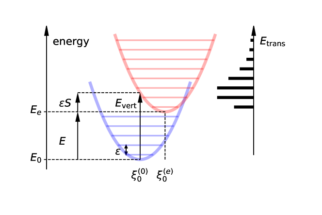
Figure 1: Displaced harmonic oscillator model for the electronic ground state (blue) and one excited state (red). The black bars on the right show the size of the squared Franck-Condon factors for a transition from the vibrational ground state.

Starting from (4) the widely used Placzek approximation is obtained by employing the semi-classical approximation⁴³ to replace the energy terms $E_{e}-E_{0}+\varepsilon^{e}_{k}-\varepsilon^{0}_{i}$ by their main contribution that is the vertical transition energy to this specific electronic state, i.e.

$$E_{e}-E_{0}+\varepsilon^{e}_{k}-\varepsilon^{0}_{i}\approx E_{{\rm vert},e}\;,$$ (6)

see Fig. 1. The vertical transition energy depends on the nuclear position and is understood to be inside of the matrix element involving the initial vibrational state $|i^{0}\rangle$. The equivalent application of a classical Wigner phase space approximation^{43, 44} leads to the same result. We will discuss the validity of this assumption further below. Applying the approximation (6) the $k$-dependence of the denominator in eq. (4) vanishes, and the closure relation within the vibrational subspace can be used¹⁸

$$\sum_{k}|k^{e}\rangle\langle k^{e}|=I_{{\rm vib},e}$$ (7)

leading to

$$V_{FI}=\langle i^{0}|\mathbf{u}_{L}\cdot\sum_{e}\left[\frac{\mathbf{m}_{e}\mathbf{m}^{*}_{e}}{E_{{\rm vert},e}-\hbar\omega_{L}}+\frac{\mathbf{m}^{*}_{e}\mathbf{m}_{e}}{E_{{\rm vert},e}+\hbar\omega_{S}}\right]\cdot\mathbf{u}_{S}|f^{0}\rangle.$$ (8)

In case of real valued wave functions (as can always be assumed the case of finite systems in absence of magnetic fields) and using $\omega_{L}\approx\omega_{S}$ in the denominator, this matrix element further reduces to

$$V_{FI}=\mathbf{u}_{L}\cdot\langle i^{0}|\alpha(\omega_{L})|f^{0}\rangle\cdot\mathbf{u}_{S}$$ (9)

where the polarizability tensor

$$\alpha(\omega)=\sum_{e}\frac{2E_{{\rm vert},e}\mathbf{m}_{e}\mathbf{m}_{e}}{E_{{\rm vert},e}^{2}-\hbar^{2}\omega^{2}}\;.$$ (10)

of the system in its electronic ground state emerges.

Eq. (9) has important consequences as it represents the overlap between initial and final vibronic states in the electronic ground state that are orthonormal. In order to get a non-vanishing vibrational contribution (apart from the Rayleigh scattering, where $f^{0}=i^{0}$), an operator depending on vibrational coordinates is required. This dependence can be extracted by expanding $\alpha(\omega)$ in terms of normal vibrational coordinates³ $Q_{v}$ around the nuclear equilibrium position $\xi_{0}$, where usually only the first order is taken into account

$$\alpha(\omega;\xi)=\alpha(\omega;\xi_{0})+\sum_{v}\left.\frac{\partial\alpha(\omega;\xi_{0})}{\partial Q_{v}}\right|_{Q_{v}=0}Q_{v}\;.$$ (11)

The first term in the expansion (11) corresponds to Rayleigh scattering and the second term contributes to the Raman effect giving

$$|V_{FI}|^{2}=\sum_{v}|\langle i^{0}|Q_{v}|f^{0}\rangle|^{2}\left|\mathbf{u}_{L}\cdot\frac{\partial\alpha(\omega_{L})}{\partial Q_{v}}\cdot\mathbf{u}_{S}\right|^{2}\;.$$ (12)

The orthogonality of the vibrational states in the electronic ground state shows that coupling to vibrational excitations is due to the first derivatives in eq. (11) only, and that only single vibrational quanta can be introduced by light scattering within this approximation. Anharmonic effects ore mode mixing^{45, 12, 13} might lead to multiple vibrational excitations. These effects are of second order in the derivative after vibrational coordinates (c.f. Fig. 2 below) and thus beyond the IMDHO model applied here.

The Placzek approximation is very successful for molecules. These have a large electronic “gap”, such that the usual experimental excitation wavelengths $\omega_{L}$ in the infrared or visible regions are far from any electronic resonances of the molecules. Many calculations even assume the limit $\omega_{L}\to 0$ and calculate $I_{\rm Ram,v}$ from the static polarizability derived by calculations with static electric fields ^{46, 47, 3, 48, 49, 50, 16, 9}. This intensity is often interpreted as “the” Raman intensity although experimental approaches report a wavelength dependence of Raman spectra since decades ²⁹.

The assumption that all electronic resonances are far from $\hbar\omega_{L}$ is not valid anymore in solids. Raman spectra are the primary source of information to characterize amorphous carbon for example, where the usual $\omega_{L}$ are well in the range of electronic excitation frequencies.⁵¹ Therefore strong effects from variations in $\omega_{L}$ are reported.⁵² This motivated Profeta and Mauri ¹⁸ to express eq. (8) as function of two independent sets of nuclear coordinates $\xi,\xi^{\prime}$ in $\mathbf{m}_{e}$ and $E_{{\rm vert},e}$, respectively. The polarizability tensor reads then

$$\alpha(\omega;\xi,\xi^{\prime})=\sum_{e}\frac{2E_{{\rm vert},e}(\xi^{\prime})\mathbf{m}_{e}(\xi)\mathbf{m}_{e}(\xi)}{E_{{\rm vert},e}^{2}(\xi^{\prime})-\hbar^{2}\omega^{2}}\;.$$ (13)

The authors give some reasoning to consider the derivatives after $\xi$ in $\mathbf{m}_{e}$, only, which obviously is only part of the contribution. We will call this contribution “Profeta” that is

$$|V_{FI}^{\rm Profeta}|^{2}=\sum_{v}|\langle i^{0}|Q_{v}|f^{0}\rangle|^{2}\left|\mathbf{u}_{L}\cdot\frac{\partial\alpha(\omega_{L};\xi,\xi^{\prime})}{\partial Q_{v}}\cdot\mathbf{u}_{S}\right|^{2}\;$$ (14)

with the vibrational coordinates $Q_{v}$ corresponding to the nuclear coordinates $\xi$. This part is labeled “three-band terms” by Wang et al.¹⁷ We name the remaining part of (8) “Pl/Pr” as shorthand for Placzek without Profeta in the following. It explicitly reads

$$|V_{FI}^{\rm Pl/Pr}|^{2}=\sum_{v}|\langle i^{0}|Q_{v}|f^{0}\rangle|^{2}\left|\mathbf{u}_{L}\cdot\frac{\partial\alpha(\omega_{L};\xi,\xi^{\prime})}{\partial Q_{v}^{\prime}}\cdot\mathbf{u}_{S}\right|^{2}\;$$ (15)

with the vibrational coordinates $Q_{v}^{\prime}$ corresponding to the nuclear coordinates $\xi^{\prime}$. This part was labeled as “two-band terms” in Wang et al.¹⁷ We will see further below that neglecting the “Pl/Pr” contribution can be a severe and misleading approximation at least in molecular systems as it disregards the resonant part of the Raman contributions.

In order to go beyond the Placzek approximation, one may start form eq. (4) where we note that in contrast to $E_{{\rm vert},e}=E_{{\rm vert},e}(\xi)$, all energies are independent of nuclear coordinates. We may expand already the matrix elements in terms of normal coordinates^{27, 53, 31}

$$\mathbf{m}_{e}(\xi)=\mathbf{m}_{e}(\xi_{0})+\sum_{v}\left.\frac{\partial\mathbf{m}_{e}}{\partial Q_{v}}\right|_{Q_{v}=0}Q_{v}\;.$$ (16)

The first term of this expansion leads to the Albrecht A term

$$V_{FI}^{A}=\sum_{e}\sum_{k}\mathbf{u}_{L}\cdot\left[\frac{\mathbf{m}_{e}\langle i^{0}|k^{e}\rangle\langle k^{e}|f^{0}\rangle\mathbf{m}_{e}}{E_{e}-E_{0}+\varepsilon^{e}_{k}-\varepsilon^{0}_{i}-\hbar\omega_{L}}+\frac{\mathbf{m}_{e}\langle i^{0}|k^{e}\rangle\langle k^{e}|f^{0}\rangle\mathbf{m}_{e}}{E_{0}-E_{e}+\varepsilon^{e}_{k}-\varepsilon^{0}_{i}+\hbar\omega_{S}}\right]\cdot\mathbf{u}_{S}$$ (17)

where we use the shorthand notation $\mathbf{m}_{e}=\mathbf{m}_{e}(\xi_{0})$. It is also called the Franck-Condon term^{54, 31} and is believed to be dominating for $\omega_{L}$ in resonance with optically strong transitions²³. Note, that a non-negligible contribution from Albrecht A to the off resonant Raman spectrum of water was reported recently.³⁰ Close to resonance often only the first part inside of the brackets is kept since this is the dominating contribution due to the small denominator. The other part is non-resonant and hence much smaller, such that

$$V^{A}_{FI}=\sum_{e}\mathbf{u}_{L}\cdot\mathbf{m}_{e}\mathbf{m}_{e}\cdot\mathbf{u}_{S}\sum_{k}\frac{\langle i^{0}|k^{e}\rangle\langle k^{e}|f^{0}\rangle}{E_{e}-E_{0}+\varepsilon^{e}_{k}-\varepsilon^{0}_{i}-\hbar\omega_{L}}$$ (18)

represents a good approximation in the neighborhood of resonances^{55, 56, 57, 36}. Eq. (18) also shows that in case of a single, isolated resonance, as it is often present in organic chromophors, the Raman cross section is mainly determined by the weighted Franck-Condon overlaps $\langle i^{0}|k^{e}\rangle\langle k^{e}|f^{0}\rangle$ corresponding to this single transition.²³

Albrecht²⁷ splits the contributions of the first derivatives in (16) into a resonant part ($B$ term)

$$V_{FI}^{B}=\sum_{e}\sum_{k}\mathbf{u}_{L}\cdot\frac{\langle i^{0}|k^{e}\rangle\langle k^{e}|Q_{v}|f^{0}\rangle\mathbf{m}_{e}\mathbf{m}^{v*}_{e}+\langle i^{0}|Q_{v}|k^{e}\rangle\langle k^{e}|f^{0}\rangle\mathbf{m}^{v}_{e}\mathbf{m}^{*}_{e}}{E_{e}-E_{0}+\varepsilon^{e}_{k}-\varepsilon^{0}_{i}-\hbar\omega_{L}}\cdot\mathbf{u}_{S}$$ (19)

and a non-resonant part ($C$ term)

$$V_{FI}^{C}=\sum_{e}\sum_{k}\mathbf{u}_{L}\cdot\frac{\langle i^{0}|k^{e}\rangle\langle k^{e}|Q_{v}|f^{0}\rangle\mathbf{m}^{v*}_{e}\mathbf{m}_{e}+\langle i^{0}|Q_{v}|k^{e}\rangle\langle k^{e}|f^{0}\rangle\mathbf{m}^{*}_{e}\mathbf{m}^{v}_{e}}{E_{e}-E_{0}+\varepsilon^{e}_{k}-\varepsilon^{0}_{i}+\hbar\omega_{S}}\cdot\mathbf{u}_{S}\;,$$ (20)

where the shorthand $\mathbf{m}^{v}_{e}=\partial\mathbf{m}_{e}/\partial Q_{v}$ is used. The sum of these two terms are labeled Albrecht $B$ term by Gong et al³⁰ and is also called Franck-Condon/Herzberg-Teller term^{54, 31}. There is also the possibility to consider both derivatives in the matrix elements. This so called Herzberg-Teller term³¹ is believed to be only important when the matrix elements vanish, i.e. for symmetry forbidden transitions ⁵⁸ and is not considered in our work.

In order to simplify the dependence on the polarization vectors $\mathbf{u}_{L}$ and $\mathbf{u}_{S}$, the so called Raman invariants¹ can be defined from the tensor elements of $\alpha^{\prime}=\partial\alpha/\partial Q_{v}$ for the Placzek approximation. These are the mean polarizability^{59, 3, 1}

$$a=\frac{1}{3}(\alpha_{xx}^{\prime}+\alpha_{yy}^{\prime}+\alpha_{yy}^{\prime})\,,$$ (21)

the anisotropy^{1, 31} (this quantity is also denoted by $\beta$^{3, 49} or $g$³⁶)

$$\gamma^{2}=\frac{1}{2}\left[|\alpha_{xx}^{\prime}-\alpha_{yy}^{\prime}|^{2}+|\alpha_{xx}^{\prime}-\alpha_{zz}^{\prime}|^{2}+|\alpha_{yy}^{\prime}-\alpha_{zz}^{\prime}|^{2}\right]+$$

$$\frac{3}{4}\left[|\alpha_{xy}^{\prime}+\alpha_{yx}^{\prime}|^{2}+|\alpha_{xz}^{\prime}+\alpha_{zx}^{\prime}|^{2}+|\alpha_{yz}^{\prime}+\alpha_{zy}^{\prime}|^{2}\right]$$ (22)

and the asymmetric anisotropy¹ (often assumed to vanish^{3, 49} as expected for non-resonant Raman², and also denoted by $d$³⁶)

$$\delta^{2}=\frac{3}{4}\left[|\alpha_{xy}^{\prime}-\alpha_{yx}^{\prime}|^{2}+|\alpha_{xz}^{\prime}-\alpha_{zx}^{\prime}|^{2}+|\alpha_{yz}^{\prime}-\alpha_{zy}^{\prime}|^{2}\right]$$ (23)

from which the absolute Raman intensity^{3, 49, 16, 36}

$$I_{\rm Ram,v}=45a^{2}+7\gamma^{2}+5\delta^{2}$$ (24)

is obtained. This intensity is usually given in units of Å${}^{4}/$amu.³ Expression (24) is valid only for the most common experimental setup and other combinations of $a,\gamma,\delta$ appear depending on the polarization of incoming and outgoing photons.¹ Similar Raman invariants can also be defined from the tensor element of the matrix element (4) instead of the polarizability derivatives $\alpha^{\prime}$.¹ The resulting expression for the intensity is similar to (24) and is called $I$ in the following. In order to directly compare $I$ and $I_{\rm Ram,v}$ one would have to multiply the latter with the vibrational matrix element (Franck-Condon factor) $|\langle i^{0}|Q_{v}|f^{0}\rangle|^{2}$. The intensity $I$ is therefore usually given in (eÅ/eV)².

In the following, we will compare Placzek and Albrecht approximations using ab-initio calculations of small molecules. This will show the similarities and differences of the two approximations. We will find that the Albrecht and its semi-classical approximation Placzek largely agree for all excitation frequencies and that in particular the approximation of Profeta corresponds to Albrecht B/C and the missing terms Pl/Pr to Albrecht A. The interested reader is also referred to Appendix A that elaborates on a clear connection between Placzek and Albrecht in the limit $\omega_{L}\to 0$.

3 Methods

The electronic structure of the systems considered here is described by density functional theory (DFT) as implemented in the GPAW software suite ^{60, 61}. The Kohn-Sham orbitals and the electronic density are described in the projector augmented wave (PAW) method ⁶² where the smooth wave functions are represented on real space grids. The exchange correlation functional is approximated in the generalized gradient correction as devised by Perdew, Burke and Ernzerhof (PBE) ⁶³. The real space grid was ensured to contain at least 4 Å of vacuum space around each atom. The grid spacing for the wave-functions was chosen to be 0.2 Å, while the density was represented on grids with 0.1 Å spacing. Molecular structures were considered to be relaxed when no force exceed 0.01 eV/Å. Vibrational modes and frequencies are calculated within the finite difference approximation of the dynamical matrix^{3, 64}. Excited state properties are calculated in time dependent DFT (TDDFT) linear response formalism as reported by Casida ^{65, 66}. The range of Kohn-Sham single-particle excitations was large enough to cover all the excitations in the energy ranges displayed, which also ensures convergence of the sum over states in polarizability derivatives and Alrecht terms. The Franck-Condon factors are calculated as described by Guthmuller. ³¹

We use the IMDHO approximation that considers only changes in excited state energies in linear order and no mixing of ground state vibrational modes, i.e. Duschinsky effects³¹ are thus not included. Derivatives of polarizabilities, transition energies and matrix elements are calculated using finite differences. Note, that this involves arbitrary phases related to the Berry phase in case of the matrix elements from eq. (16) and therefore needs special care as discussed in appendix C.

4 Results

Molecular hydrogen is the simplest existing neutral molecule and serves as a good example to show the basic properties and consequences of the different approximations for obtaining Raman intensities described above. There is only one vibrational mode in H₂ which is found in our calculation at 4337 cm^-1 = 0.538 eV in fair agreement to the exact value of 4163.3 cm^-1.⁶⁷

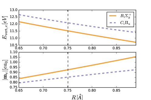
Figure 2: Electronic transition energies $E_{{\rm vert},e}$ and transition dipoles from the ground ${}^{1}\Sigma_{u}^{+}$ state to $B^{1}\Sigma_{g}^{+},C^{1}\Pi_{u}$ states of the H₂ molecule depending on the nuclear distance $R$. Vertical lines indicate the equilibrium distance.

The main ingredients determining Raman intensities are the derivatives of transition energy and dipole matrix element with respect to the normal coordinate of the corresponding vibration in Eqs. (11) and (16). Fig. 2 shows these quantities for the first two optically allowed transitions in the H₂ molecule in dependence of the bond length $R$. Both quantities depend linearly on $R$ in agreement with the literature ^{68, 69}. Adding a linear function to a Harmonic potential does only change the potential minimum, but not its form, i.e. the vibrational frequencies in ground and excited state are the same (see also appendix B). Therefore the displaced harmonic oscillator model underlying the definition of the Huang-Rhys parameter ⁷⁰ is indeed justified here. Taking into account only the linear term in a Taylor expansion of the energy around the equilibrium position in the normal modes leads to the displaced harmonic oscillator model depicted in Fig. 1.

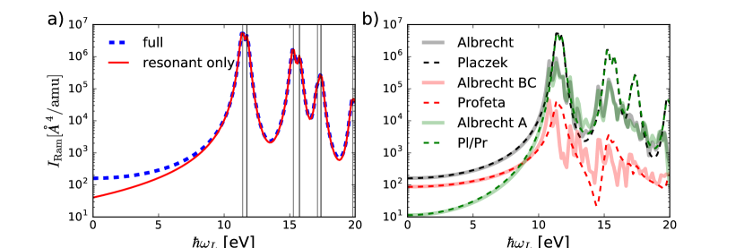
Figure 3: a) Full Placzek Raman intensity for H₂ compared to the resonant term only. Vertical lines show optically active transitions with oscillator strength $f\geq 0.01$. b)Raman intensity from different approximations. A width of $\gamma=0.2$ eV is applied for Placzek like approximations and $\gamma=0.1$ eV for Albrecht terms.

Fig. 3 a) shows the absolute Raman intensity in logarithmic scale as a function of the excitation frequency $\omega_{L}$. The Raman intensity display a rather smooth dependence on photon energy for small $\hbar\omega_{L}$, i.e. if $\hbar\omega_{L}\ll E_{e}$ for all optically strong electronic transitions energies $E_{e}$ in the system. In contrast, the intensity gets strongly peaked close to the transition energies if there is sufficient oscillator strength in the corresponding transitions. A finite width $\gamma$ is added as complex energy to the full range of $\hbar\omega_{L}$ effectively broadening these peaks. Fig. 3 a) also compares the contributions of the resonant and non-resonant terms in eq. (8). The non-resonant part can indeed be neglected, except when approaching the static limit $\hbar\omega_{L}\to 0$, where the non-resonant part is needed to get full intensity.

A comparison of the different approximations and their contributions for H₂ is depicted in Fig. 3 b). We report the absolute Raman intensity although the Albrecht terms do not contain the factor $|\langle i^{0}|Q_{v}|f^{0}\rangle|^{2}$ in eq. (12). The Albrecht matrix elements have been divided by this factor to get comparable numbers. Concentrating on the full Albrecht and Placzek approximation first, the similarity and even overlap of the two approximations for small $\omega_{L}$ far from the resonances becomes apparent. The two approximations yield the same result in a wide energy range and there is even a qualitative similarity in the resonance regions. The main difference is that the less approximate Albrecht approximation leads to many more peaks than Placzek. The Placzek peaks are at the semi-classical vertical transition energies where the denominator in eq. (8) diverges. In contrast, the Albrecht terms exhibit peaks at each of the phonon decorated electronic excitations in the denominators of A, B and C terms in Eqs. (17-20). For this reason we had to apply twice the broadening $\gamma$ in the narrower peaks of Placzek as compared to Albrecht.

	full	Albrecht A or Pl/Pr	Albrecht BC or Profeta
Albrecht	191	11.5	109
Placzek	188	11.4	107

Table 1: Static ($\omega_{L}=0$) absolute Raman intensities for the H₂ molecule in Å${}^{4}/$amu.

Interestingly, and in agreement with the considerations of appendix A, the Profeta approximation turns out to be the semi-classical approximation of the Albrecht BC terms. The term missing in Profeta treatment corresponds to the Albrecht A term. The connections and agreement between Albrecht and Placzek, and Albrecht BC and Profeta are further corroborated by the numerical values for static Raman intensities listed in tab. 1. As expected, the Albrecht BC terms dominate for small $\omega_{L}$, but these terms are not enough to give the full intensity. Even in the limit $\hbar\omega_{L}/E_{e}\to 0$ the consideration of the Albrecht A contribution is important and cannot be neglected. Albrecht A clearly dominates in the resonance region and is the main contribution to the full Raman intensity. In certain energy regions the Albrecht A intensity is even larger than full Albrecht, which indicates destructive interference with the Albrecht BC terms. We note that there is no energy region where Albrecht BC (and Profeta) is sufficient to give the correct intensities. Placzek generally provides a good coarse grained description of the intensity behavior as compared to Albrecht, however.

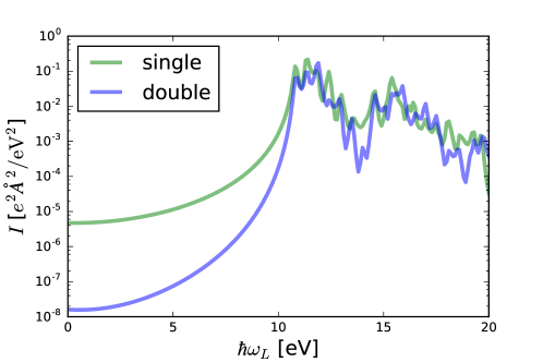
Figure 4: Single and double vibrational excitation intensities according to the Albrecht A term in the H₂ molecule. A width of $\gamma=0.1$ eV is applied.

Now we turn to multiple vibrational excitations, the so called overtones and combinations bands in contrast to the fundamentals that correspond to single excitations. ⁴² Here, we expect severe difference between Albrecht and Placzek approximations since they are impossible in Placzek within the IMDHO approximation. As an example, the intensity of double vibrational excitation in the Albrecht A term of H₂ is compared to the single excitation Albrecht A term in Fig. 4. For low excitation energies and thus far from resonance, the intensity of vibrational double excitation is several orders of magnitude smaller than that of a single excitation. This changes drastically near to resonances, where the intensities become the same size and the intensity of the vibrational double excitation can even overbalance that of the single excitation.

	$\omega_{v}$		$I_{\rm Ram}(0)$		$I_{\rm Ram}(\omega_{L}^{\rm exp}\equiv 514.5{\rm nm})$
mode	ours	exp.	ours	others	ours	others	exp.f
$v_{2}(1A_{1})$	1585	1595a, 1638b	1.4	0.8c, 0.9d, 1.1e	1.4	1.1e	0.9$\pm$0.2
$v_{1}(2A_{1})$	3747	3657a, 3832b	112	109c, 120d, 111e	127	129e	108$\pm$14
$v_{3}(1B_{2})$	3846	3756a, 3943b	25	26c, 30d, 26e	28	29e	19.2$\pm$2.1

^aexp. vapor⁷¹, ^bexp. harmonic⁷², ^cPW92³, ^dBP86⁷³, ^ePBE⁷⁴, ^ffrom ref. ⁴⁷

Table 2: Vibrational frequencies in cm^-1 and Placzek absolute Raman intensities for $\hbar\omega_{L}/E_{e}\to 0$ in Å${}^{4}/$amu. A width of $\gamma=0.2$ eV is applied for the calculations at $\omega_{L}^{\rm exp}$.

Next we consider the water molecule. We first discuss the results in the limit $\hbar\omega_{L}/E_{e}\to 0$ where several other calculations and extensive experimental data (for small $\hbar\omega_{L}$) are available. The gas-phase water molecule has three independent vibrational modes that are all Raman active. Table 2 shows the good agreement of our calculated absolute Raman intensities in this limit both with experiment as well as with other calculations. There are differences due to different density functionals applied, but all approaches are of roughly the same good accuracy as compared to experiment. Static and dynamic polarizabilities for the experimental wavelength of 514.5 nm (2.41 eV) lead to small differences ⁷⁴, only. While the very weak Raman intensity of $v_{2}$ does not change, the stronger $v_{1}$ and $v_{3}$ slightly increase.

mode	exp47	Albrecht	Albrecht 30	Albr. $A$	Albr. $A$ 30	$B+C$	$B+C$ 30
$v_{2}$	0.9	2.7	1.1	0.5	0.1	5.3	1.5
$v_{1}$	108	103	105	7.6	11.7	56	48.3
$v_{3}$	19.2	30	25.7	0	0	30	25.7

Table 3: Absolute Raman intensities for $\omega_{L}=0$ in the Albrecht approximations from our calculations and from Gong et al.³⁰ in Å${}^{4}/$amu.

Table 3 lists the static ($\omega_{L}\to 0$) absolute Raman contributions from the Albrecht terms. Our calculation agrees well with the the recent results of Gong et al.³⁰ and we confirm that the Albrecht A term cannot be neglected in this limit for $v_{1}$ and $v_{2}$.

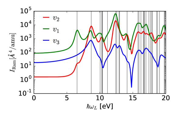
Figure 5: Frequency dependent Placzek-Raman intensities of the three vibrations in water. A width of $\gamma=0.2$ eV is applied. Optically active transitions with $f\geq 0.02$ are marked by gray lines.

Next we increase the energy of the incoming photon to the resonance region as shown in Fig. 5, where $I_{\rm Ram}$ is depicted on logarithmic scale in the region up to 20 eV. There are dramatic changes in the relative intensities. Coming from small $\omega_{L}$ all three vibrations show increasing intensity when entering the resonance region. The behavior of the three vibrations is very different, however. While $v_{1}$ and $v_{2}$ show a clear peak at the first optically active transition, $v_{3}$ is unaffected. Interestingly, vibration $v_{1}$, that is extremely weak in the limit $\omega_{L}\to 0$ increases most rapidly and even gets the highest contribution around 9 eV. The deep minima in the intensities visible in particular for $v_{3}$ indicate destructive interference that strongly affects the intensity.

Finally we present the non-resonant and near-resonant Raman spectra of trans-butadiene where experimental non-resonant⁷⁵ resonant⁷⁶ Raman spectra as well as an early theoretical investigation within the Albrecht approximation²⁵ are available. Duschinsky effects have been reported in this molecule ⁷⁷ and these are important to understand the fluorescence quantum efficiency.^{78, 79} The neglect of mode mixing as in the IMDHO model applied here has been reported to capture the geometry changes in the main optical $1^{1}A_{g}^{-}\to^{1}B_{u}^{+}$ transition,⁸⁰ however. In the experiment this transition is found at 5.92 eV. Our calculated value (5.53 eV) is lower than the experimental one as well as the transition energy in higher level quantum chemistry methods⁸¹. The oscillator strength is 0.68, which is higher than the experimental value of 0.4⁸², but in concord with other computations⁸². The underestimation of excitation energies in GGAs is well known⁸³, while the rather accurate oscillator strength indices a qualitatively correct description of the nature of the excitation. In order to compare our resonant Raman calculations to experiment we have to take account of the differences in excitation energies. Multiple vibrational excitations appear only if there is a nearby resonance and their contribution crucially depends on the energetic distance between $\hbar\omega_{L}$ and $E_{I}$ as we have seen in Fig. 4 for H₂. In the following we calculate our spectra at 5.92 eV - 5.53 eV = 0.39 eV lower excitation energies than in experiment in order to be at the same energetic distance from the main optical resonance.

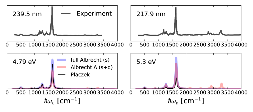
Figure 6: Near resonant ($\hbar\omega_{L}=5.3$ eV $\mathrel{\widehat{=}}$ 217.9 nm, see text) and more off-resonant ($\hbar\omega_{L}=4.79$ eV $\mathrel{\widehat{=}}$ 239.5 nm) Raman spectra for trans-butadiene in comparison to the experimental spectra of Chadwick et al.⁷⁶ The spectrum labeled full Albrecht (s) contains all Albrecht A-C terms for single vibrational contributions, while the Albrecht A (s+d) term contains vibrational double excitations also. A width of $\gamma=0.2(0.4)$ eV was applied to Albrecht(Placzek) approximations and the intensities were folded by Lorentzians of 50 cm^-1 width.

Experimental and calculated spectra related in this way closely resemble each other as is shown in Fig. 6. The spectrum in the non-resonant region (at 4.79 eV in our calculation corresponding to 239.5 nm or 5.18 eV experimentally) has significant contribution from the Albrecht B and C terms and there is nearly no intensity above 2000 cm^-1. In this frequency range the Placzek approximation gives a good description of the spectrum. Apart from the main peak at 1645 cm^-1 also other small peaks at lower vibrational energies appear in the calculation similar to experiment as further detailed in Tab. 4 below. This changes near to resonance (5.30 eV in our calculation corresponding to 217.9 nm or 5.69 eV experimentally), where Albrecht A practically determines the full intensity. The Placzek approximation gives much lower intensity as compared to Albrecht. There are also contributions of higher excitations due to the dominating Albrecht A term that naturally appear at higher vibrational frequencies. These are completely neglected within the Placzek approximation.

$\hbar\omega_{v}$	$\hbar\omega_{v}$ (exp)	assignment	$I^{\rm Albrecht}$	$I^{\rm Placzek}$	$I^{\rm AlbrechtA}$	$I^{\rm Albrecht,c}$
502	513a, 508b	$v_{9}$ $\beta$(CCC)	4.1	3.8	3.9	0.2
879	910a, 890b	$v_{8}$ $\gamma$(C-C), $\beta$(H)	0.8	1.1	1.9	1.3
1195	1204a, 1200b	$v_{7}$ $\gamma$(C-C)	2.3	3.0	1.4	40.3
1272	1279a, 1279b	$v_{6}$ $\beta$(H)	14.1	16.9	15	0.7
1275		$\beta$(H)	1.4	1.8	1.4	-
1424	1442a, 1442b	$v_{5}$ $\beta$(H)	1.3	1.7	0.7	0.3
1645	1643a, 1642b	$v_{4}$ $\gamma$(C-C,C=C)	100(0.87)	100(0.31)	100(0.7)	100
2917	2879a	$v_{4}+v_{6}$	-	-	10.7	-
3290	3267a	2$v_{4}$	-	-	23.2	-

^aexperiment of Richards and Nielsen⁷⁵, ^bexperiment of Chadwick et al.⁷⁶, ^c non-resonant ($\hbar\omega_{L}=$1.24 eV) Albrecht from Warshel and Dauber²⁵

Table 4: Vibrational energies (in cm${}^{-}1$) and relative intensities of the most active Raman lines. The intensity of the strongest line in $e^{4}\rm{\AA}^{4}/$eV² is given in brackets. Assignment of modes follows Chadwick et al.⁷⁶, and $\beta,\gamma$ represent in-plane bending and stretching modes, respectively. Numerical settings as in Fig. 6.

The Raman peaks and their intensities are further detailed in tab. 4. As suggested from Fig. 6 our vibrational energies are in good agreement to experiment. There are two in-plane H-bending modes at 1272 cm^-1 and 1275 cm^-1 that are probably hard to resolve in the experiment. One of them is the second most intense line in our calculations, while the strong Raman excitation of the 1195 cm^-1 found in the calculations of Warshel and Dauber²⁵ cannot be confirmed by us (further off-resonant spectra resemble the 4.79 eV spectrum in Fig. 6). Interestingly, the Placzek approximation gives relative intensities in good agreement to Albrecht despite its much lower absolute intensity.

5 Conclusions

We have shown in this contribution how the Placzek and Albrecht terms can be derived from the photon scattering matrix elements in the formulation by Kramers, Heisenberg and Dirac. The widely used Placzek approximation is found to represent the semi-classical limit of the more exact Albrecht formulation. While the excitation energy-dependent peak structure is much simpler in the Placzek approximation, the overall behavior of the Raman intensities is remarkably similar to Albrecht also in resonance regions for the molecules investigated. The similarity breaks down for multiple excitations of vibrational modes appearing as soon as the photon energy approaches the resonance region. These are forbidden in the Placzek form within the independent mode double harmonic approximation, but are well described within the Albrecht approximation.

6 Acknowledgment

MW thanks J. Guthmuller for useful discussion. Support by ASTC is gratefully acknowledged. We are grateful for computational resources from FZ-Jülich and from the Nemo cluster at the University of Freiburg.

Appendix A Connection between Placzek and Albrecht approximations for $\omega_{L}\to 0$

We consider the limit of very small excitation energies $\hbar\omega_{L}$, where small means far from any electronic resonance in the system. This limit can formally be described by $\omega_{L}\to 0$. However, this is a formal limit only, as scattering of zero frequency photons is meaningless. Both Placzek and Albrecht approximations should be valid in this limit and the approximations indeed coincide as we will show in the following.

The polarizability tensor (10) in this limit simplifies to ⁴⁶

$$\alpha(\omega=0)=\sum_{e}\frac{2m_{L}^{e}m_{S}^{e}}{E_{{\rm vert},e}}\;.$$ (25)

This tensor enters the Placzek approximation via its derivatives with respect to vibrational coordinates. Nonzero derivatives arise from two distinct sources: Either from the transition energy $E_{{\rm vert},e}$ or from the matrix elements $m_{L,S}^{e}$. Without loss of generality, we consider only a single electronic excited state and thus suppress the label $e$ for brevity in the following. The explicit derivative is then

$$\frac{\partial\alpha}{\partial Q}=\frac{2}{E_{\rm vert}}\left[m_{S}m_{L}^{\prime}+m_{L}m_{S}^{\prime}\right]-2m_{S}m_{L}\frac{E_{\rm vert}^{\prime}}{E_{\rm vert}^{2}}\;,$$ (26)

where the prime denotes the derivative with respect to a nuclear coordinate.

In order to show the equivalence to the Albrecht approximation for $\omega_{L}\to 0$, we will discuss the different terms appearing in (26) separately and show that these correspond to the different terms in the Albrecht approximation, i.e. we will show that in the limit of small $\omega_{L}$

$$V^{A}\approx-\langle 0^{0}|Q|1^{0}\rangle 2m_{S}m_{L}\frac{E_{\rm vert}^{\prime}}{E_{\rm vert}^{2}}$$ (27)

and

$$V^{B}+V^{C}\approx\langle 0^{0}|Q|1^{0}\rangle\frac{2}{E_{\rm vert}}\left[m_{S}m_{L}^{\prime}+m_{L}m_{S}^{\prime}\right]$$ (28)

hold.

We first discuss the Albrecht B term, defined by eq. (19), which becomes in the limit of $\hbar\omega_{L}/E\to 0$

$$V^{B}=m_{S}m_{L}^{\prime}\sum_{k}\frac{\langle 0^{0}|Q|k\rangle\langle k|1^{0}\rangle}{E+k\varepsilon}+m_{S}m_{L}^{\prime}\sum_{k}\frac{\langle 0^{0}|k\rangle\langle k|Q|1^{0}\rangle}{E+k\varepsilon}\;$$ (29)

Replacing the denominator $E+k\varepsilon$ by the vertical transition energy $E_{\rm vert}$ and applying the completeness relation eq. (7) leads to

$$V^{B}=\frac{1}{E_{\rm vert}}\left[m_{S}m_{L}^{\prime}+m_{L}m_{S}^{\prime}\right]\langle 0^{0}|Q|1^{0}\rangle$$ (30)

which is the half of the first term in eq. (28). The other half is given by $V^{C}$ within the same approximation.

To prove (27) we consider real matrix elements

$$V^{A}=m_{L}m_{S}\sum_{k}\langle 0^{0}|k\rangle\langle k|1^{0}\rangle\left[\frac{1}{E+k\varepsilon-\omega_{L}}+\frac{1}{E+k\varepsilon+\omega_{S}}\right]\;,$$ (31)

use $\omega_{S}\approx\omega_{L}$, $\omega_{L}\to 0$ and expand in $\epsilon/E$ up to first order, which leads to

$$V^{A}=2m_{L}m_{S}\sum_{k}\langle 0^{0}|k\rangle\langle k|1^{0}\rangle\frac{1}{E}\left(1-k\frac{\varepsilon}{E}\right)$$ (32)

The first term in brackets vanishes due to orthogonality of $\langle 0^{0}|1^{0}\rangle$ (after closure in $k^{e}$) and one can show that

$$\sum_{k}\langle 0^{0}|k\rangle k\langle k|1^{0}\rangle=-\frac{\Delta}{\sqrt{2}}$$ (33)

where the dimensionless displacement

$$\Delta=\sqrt{\frac{\mu\omega}{\hbar}}\left(\xi_{0}^{(e)}-\xi_{0}^{(0)}\right)$$ (34)

appears (c.f. Fig. 1). One can further show that

$$\langle 0^{0}|Q|1^{0}\rangle E_{\rm vert}^{\prime}=\sqrt{\frac{\hbar}{2\omega}}\left(-\varepsilon\Delta\sqrt{\frac{\omega}{\hbar}}\right)$$ (35)

such that eq. (32) can be written

$$V^{A}\approx-2m_{L}m_{S}\frac{E_{\rm vert}^{\prime}}{E_{\rm vert}^{2}}$$ (36)

where $E\approx E_{\rm vert}$ entered. This finally proofs the approximate equality of Placzek and Albrecht approximations in the limit $\omega_{L}\to 0$.

Appendix B Taylor expansion and displaced harmonic oscillator

Franck-Condon factors can be efficiently calculated within the double harmonic approximation. Deviations from this approximation, the Herzberg-Teller and Duschinsky effects are usually rather small⁸⁴. This property can be understood by expanding the possible effects in a series in the displacement between ground and excited state equilibria $\rho_{0}$ and $\rho_{e}$ of some vibrational coordinate $\rho$. The ground state potential in the harmonic approximation is given by

$$E_{0}(\rho)=E_{0}(\rho_{0})+\frac{1}{2}\mu\omega^{2}(\rho-\rho_{0})^{2}\;,$$ (37)

where $\mu$ is the effective mass and $\omega$ the corresponding frequency of the harmonic potential. We may expand the excited state energy around $\rho_{0}$ in a Taylor series up to first order

$$E_{e}(\rho)=E_{e}(\rho_{0})+\left.\frac{\partial E_{e}(\rho)}{\partial\rho}\right|_{\rho=\rho_{0}}(\rho-\rho_{0})+O[(\rho-\rho_{0})^{2}]$$ (38)

Adding Eqs. (37) and (38) immediately leads to the similar harmonic equation in the excited state

$$E_{e}(\rho)=E_{e}(\rho_{0})+\frac{1}{2}\mu\omega^{2}(\rho-\rho_{e})^{2}$$ (39)

where we have identified $\rho_{e}=\rho_{0}-\frac{\partial E_{e}(\rho)}{\partial\rho}/(\mu\omega^{2})$. Thus the leading term in eq. (38) changes the equilibrium position, but not the vibrational frequency⁸⁵.

Appendix C Matrix element derivatives and the Berry phase

The evaluation of Albrecht B and C terms requires derivatives of transition dipoles with respect to nuclear coordinates. An evaluation of such derivatives in finite differences is not straightforward as it involves arbitrary phases that are present in eigenstates of parameter dependent Hamiltonians and are connected to the Berry phase ^{86, 87}. Similar problems are also present in the evaluation of hopping matrix elements ⁸⁸.

The nature of the problem and its solution can be exemplified in one dimension involving a single electronic positional coordinate $x$. An electron might be subject to a parameter dependent Hamiltonian $H(R)$, where in $R$ in our case is a nuclear coordinate. The aim is to calculate the derivative of an normalized eigenstate $f_{i}(x;R)$ of $H(R)$ with respect to the $R$ in a finite difference expression

$$dR\frac{\partial f_{i}(x;R)}{\partial R}=f_{i}(x;R+dR)-f_{i}(x;R)\;.$$ (40)

In practical calculations the evaluation of eigenstates at different $R$ are independent of each other⁸⁸. Then every eigenstate $\bar{f}_{i}(x;R+dR)=uf_{i}(x;R+dR)$ with $|u|^{2}=1$ is a perfectly valid eigenstate of $H(R+dR)$ and equally relevant as $f_{i}(x;R+dR)$ itself. The phase $u$ can spoil the derivative if $\bar{f}$ is used instead of $f$ in expression (40), however. To recover $f_{i}(x;R+dR)$ we have to apply

$$dR\frac{\partial f_{i}(x;R)}{\partial R}=u^{*}\bar{f}_{i}(x;R+dR)-f_{i}(x;R)$$ (41)

instead, where we correct for the arbitrary phase $u$. The value of this phase factor is reconstructed by using the orthogonality of $f_{i}$ and $\partial f_{i}/\partial R$ ⁸⁶ that is required for normalized states. It leads to

$$u=\int dx\,f^{*}(x;R)\bar{f}(x;R+dR)\;.$$ (42)

We have to be slightly more careful in the case of energetically degenerate states, that are common in molecules. Here, not only a phase $u$ may appear, but the states may also mix. More generally we are faced with

$$\bar{f}_{i}(x;R+dR)=\sum_{j}u_{ij}f_{j}(x;R+dR)$$ (43)

where the matrix $u$ is unitary, but arbitrary otherwise. It might be sparse, but generally not diagonal. Similar to (42) the matrix elements of $u$ can be reconstructed from

$$u_{ij}=\int dx\,f_{j}^{*}(x;R)\bar{f}_{i}(x;R+dR)$$ (44)

when terms containing $dR$ are neglected, i.e. we assume that the matrix $u$ does not change due to the small displacement. This leads to the generalized finite difference equation save from arbitrary phases

$$dR\frac{\partial f(x;R)}{\partial R}=u^{H}\bar{f}(x;R+dR)-f(x;R)\;.$$ (45)

where $f$ is the vector of eigenstates $f_{i}$, $\bar{f}$ is the vector of eigenstates $\bar{f}_{j}$ and the superscript $H$ denotes the Hermitian conjugate.

Similar to the Eigenstates discussed so far, we want to obtain derivatives of transition dipole matrix elements $m_{i\alpha}(R)=\langle f_{i}(x;R)|\hat{o}|f_{\alpha}(x;R)\rangle$ in a finite difference expression through

$$dR\frac{\partial m_{i\alpha}(R)}{\partial R}=m_{i\alpha}(R+dR)-m_{i\alpha}(R)\;,$$ (46)

where $i,\alpha$ are the indices of occupied and empty orbitals, respectively. The transition dipoles are calculated in an independent calculation again and thus are mixed and contain arbitrary phases inherited from the orbitals. We may correct for this similar to eq. (45) and write

$$dR\frac{\partial m_{i\alpha}(R)}{\partial R}=\langle\left[u^{H}\bar{f}(R+dR)\right]_{i}|\hat{o}|\left[u^{H}\bar{f}(R+dR)\right]_{\alpha}\rangle-m_{i\alpha}(R)$$ (47)

or in vector form

$$dR\frac{\partial m(R)}{\partial R}=U^{H}\bar{m}(R+dR)-m(R)$$ (48)

with

$$U_{i\alpha,j\beta}=u_{ij}^{*}u_{\alpha\beta}$$ (49)

and $\bar{m}_{i\alpha}(R+dR)=\langle\bar{f}_{i}(x;R+dR)|\hat{o}|\bar{f}_{\alpha}(x;R+dR)\rangle$.

A new class of phases appears in linear response TDDFT where the eigenvalue equation^{89, 66}

$$\Omega F_{I}=\omega_{I}^{2}F_{I}$$ (50)

is solved at each position independently. The $\omega_{I}$ denote transition energies and the eigenvectors $F_{I}$ may contain arbitrary phases and might be mixed. The matrix elements are then

$$M_{I}=\sum_{i\alpha}\sqrt{\frac{\varepsilon_{\alpha}-\varepsilon_{i}}{\omega_{I}}}(F_{I})_{i\alpha}m_{i\alpha}$$ (51)

with the single particle energies $\varepsilon_{i,\alpha}$. The $F_{I}$ at equilibrium position and the $\bar{F}_{J}$ at a displaced position are given in the corresponding particle-hole basis that we may contract to single indices $p=(i\alpha),q=(j,\beta)$ to simplify the notation. We may define an overlap similar to Eqs. (44) and (49)

$$W_{IJ}=\sum_{p,q}(\bar{F}_{J})_{p}U_{pq}(F_{I})_{q}^{*}$$ (52)

where the $U_{pq}$ are needed to connected the two particle-hole bases. This matrix connects the different linear response transition matrix elements via $\bar{M}=WM$, where

$$\bar{M}_{I}=\sum_{i\alpha}\sqrt{\frac{\varepsilon_{\alpha}-\varepsilon_{i}}{\omega_{I}}}(\bar{F}_{I})_{i\alpha}\bar{m}_{i\alpha}\;.$$ (53)

Note, that the phases of $\bar{F}$ and $\bar{m}$ are both arbitrary and independent of each other. Derivatives of linear response dipole matrix elements are finally obtained as

$$dR\frac{\partial M(R)}{\partial R}=W^{H}\bar{M}(R+dR)-m(R)\;.$$ (54)

References

- Derek A. Long 2002 Derek A. Long, The Raman Effect: A Unified Treatment of the Theory of Raman Scattering by Molecules; John Wiley & Sons Ltd, Baffins Lane, Chichester, West Sussex PO19 1UD, England, 2002
- John R. Ferraro et al. 2003 John R. Ferraro,; Kazuo Nakamoto,; Chris W. Brown, Introductory Raman Spectroscopy (Second Edition); Elsevier Inc., 2003
- Porezag and Pederson 1996 Porezag, D.; Pederson, M. R. Infrared intensities and Raman-scattering activities within density-functional theory. Physical Review B 1996, 54, 7830–7836
- Yamakita et al. 2007 Yamakita, Y.; Kimura, J.; Ohno, K. Molecular vibrations of [n]oligoacenes (n=2-5 and 10) and phonon dispersion relations of polyacene. The Journal of Chemical Physics 2007, 126, 064904
- Castiglioni et al. 2004 Castiglioni, C.; Tommasini, M.; Zerbi, G. Raman spectroscopy of polyconjugated molecules and materials: confinement effect in one and two dimensions. Philosophical Transactions of the Royal Society of London A: Mathematical, Physical and Engineering Sciences 2004, 362, 2425–2459
- Rouillé et al. 2008 Rouillé, G.; Jäger, C.; Steglich, M.; Huisken, F.; Henning, T.; Theumer, G.; Bauer, I.; Knölker, H.-J. IR, Raman, and UV/Vis Spectra of Corannulene for Use in Possible Interstellar Identification. ChemPhysChem 2008, 9, 2085–2091
- Zhao et al. 2006 Zhao, L. L.; Jensen, L.; Schatz, G. C. Surface-Enhanced Raman Scattering of Pyrazine at the Junction between Two Ag20 Nanoclusters. Nano Letters 2006, 6, 1229–1234
- Martin et al. 2015 Martin, E. J. J.; Bérubé, N.; Provencher, F.; Côté, M.; Silva, C.; Doorn, S. K.; Grey, J. K. Resonance Raman spectroscopy and imaging of push–pull conjugated polymer–fullerene blends. Journal of Materials Chemistry C 2015, 3, 6058–6066
- Vecera et al. 2017 Vecera, P.; Chacón-Torres, J. C.; Pichler, T.; Reich, S.; Soni, H. R.; Görling, A.; Edelthalhammer, K.; Peterlik, H.; Hauke, F.; Hirsch, A. Precise determination of graphene functionalization by in situ Raman spectroscopy. Nature Communications 2017, 8, 15192
- Corni et al. 2001 Corni, S.; Cappelli, C.; Cammi, R.; Tomasi, J. Theoretical Approach to the Calculation of Vibrational Raman Spectra in Solution within the Polarizable Continuum Model. The Journal of Physical Chemistry A 2001, 105, 8310–8316
- Cheeseman and Frisch 2011 Cheeseman, J. R.; Frisch, M. J. Basis Set Dependence of Vibrational Raman and Raman Optical Activity Intensities. Journal of Chemical Theory and Computation 2011, 7, 3323–3334
- Barone et al. 2014 Barone, V.; Biczysko, M.; Bloino, J. Fully anharmonic IR and Raman spectra of medium-size molecular systems: accuracy and interpretation. Phys. Chem. Chem. Phys. 2014, 16, 1759–1787
- Bloino et al. 2015 Bloino, J.; Biczysko, M.; Barone, V. Anharmonic Effects on Vibrational Spectra Intensities: Infrared, Raman, Vibrational Circular Dichroism, and Raman Optical Activity. The Journal of Physical Chemistry A 2015, 119, 11862–11874
- Ambrosch-Draxl et al. 2002 Ambrosch-Draxl, C.; Auer, H.; Kouba, R.; Sherman, E. Y.; Knoll, P.; Mayer, M. Raman scattering in YBa2Cu3O7: A comprehensive theoretical study in comparison with experiments. Physical Review B 2002, 65, 064501
- Gillet et al. 2013 Gillet, Y.; Giantomassi, M.; Gonze, X. First-principles study of excitonic effects in Raman intensities. Physical Review B 2013, 88, 094305
- Li Niu et al. 2008 Li Niu,; Jiaqi Zhu,; Wei Gao,; Aiping Liu,; Xiao Han,; Shanyi Du, First-principles calculation of vibrational Raman spectra of tetrahedral amorphous carbon. Physica B: Condensed Matter 2008, 403, 3559–3562
- 17 Wang, Y.; Carvalho, B. R.; Crespi, V. H. Strong exciton regulation of Raman scattering in monolayer MoS2. 98, 161405
- Profeta and Mauri 2001 Profeta, M.; Mauri, F. Theory of resonant Raman scattering of tetrahedral amorphous carbon. Physical Review B 2001, 63, 245415
- Stock and Domcke 1990 Stock, G.; Domcke, W. Theory of resonance Raman scattering and fluorescence from strongly vibronically coupled excited states of polyatomic molecules. The Journal of Chemical Physics 1990, 93, 5496–5509
- Peticolas and Rush 1995 Peticolas, W. L.; Rush, T. Ab initio calculations of the ultraviolet resonance Raman spectra of uracil. Journal of Computational Chemistry 1995, 16, 1261–1270
- Jarzecki and Spiro 2001 Jarzecki, A. A.; Spiro, T. G. Ab initio computation of the UV resonance Raman intensity pattern of aqueous imidazole. Journal of Raman Spectroscopy 2001, 32, 599–605
- Neugebauer and Hess 2004 Neugebauer, J.; Hess, B. A. Resonance Raman spectra of uracil based on Kramers–Kronig relations using time-dependent density functional calculations and multireference perturbation theory. The Journal of Chemical Physics 2004, 120, 11564–11577
- Scholz et al. 2011 Scholz, R.; Gisslén, L.; Schuster, B.-E.; Casu, M. B.; Chassé, T.; Heinemeyer, U.; Schreiber, F. Resonant Raman spectra of diindenoperylene thin films. The Journal of Chemical Physics 2011, 134, 014504
- Balakrishnan et al. 2012 Balakrishnan, G.; Jarzecki, A. A.; Wu, Q.; Kozlowski, P. M.; Wang, D.; Spiro, T. G. Mode Recognition in UV Resonance Raman Spectra of Imidazole: Histidine Monitoring in Proteins. The Journal of Physical Chemistry B 2012, 116, 9387–9395
- Warshel and Dauber 1977 Warshel, A.; Dauber, P. Calculations of resonance Raman spectra of conjugated molecules. The Journal of Chemical Physics 1977, 66, 5477–5488
- Albrecht 1960 Albrecht, A. C. “Forbidden” Character in Allowed Electronic Transitions. The Journal of Chemical Physics 1960, 33, 156–169
- Albrecht 1961 Albrecht, A. C. On the Theory of Raman Intensities. The Journal of Chemical Physics 1961, 34, 1476–1484
- Albrecht and Hutley 1971 Albrecht, A. C.; Hutley, M. C. On the Dependence of Vibrational Raman Intensity on the Wavelength of Incident Light. The Journal of Chemical Physics 1971, 55, 4438–4443
- Myers Kelley 2008 Myers Kelley, A. Resonance Raman and Resonance Hyper-Raman Intensities: Structure and Dynamics of Molecular Excited States in Solution. The Journal of Physical Chemistry A 2008, 112, 11975–11991
- Gong et al. 2015 Gong, Z.-Y.; Tian, G.; Duan, S.; Luo, Y. Significant Contributions of the Albrecht’s A Term to Nonresonant Raman Scattering Processes. Journal of Chemical Theory and Computation 2015, 11, 5385–5390
- Guthmuller 2016 Guthmuller, J. Comparison of simplified sum-over-state expressions to calculate resonance Raman intensities including Franck-Condon and Herzberg-Teller effects. The Journal of Chemical Physics 2016, 144, 064106
- Eric J. Heller et al. 2016 Eric J. Heller,; Yuan Yang,; Lucas Kocia,; Wei Chen,; Shiang Fang,; Mario Borunda,; Efthimios Kaxiras, Theory of Graphene Raman Scattering. ACS Nano 2016, 10, 2803–2818
- Duan et al. 2016 Duan, S.; Tian, G.; Luo, Y. Theory for Modeling of High Resolution Resonant and Nonresonant Raman Images. Journal of Chemical Theory and Computation 2016, 12, 4986–4995
- Hu et al. 2017 Hu, W.; Duan, S.; Luo, Y. Theoretical modeling of surface and tip-enhanced Raman spectroscopies. WIREs Comput Mol Sci 2017, 1293
- Avila Ferrer et al. 2013 Avila Ferrer, F. J.; Barone, V.; Cappelli, C.; Santoro, F. Duschinsky, Herzberg–Teller, and Multiple Electronic Resonance Interferential Effects in Resonance Raman Spectra and Excitation Profiles. The Case of Pyrene. Journal of Chemical Theory and Computation 2013, 9, 3597–3611
- Baiardi et al. 2015 Baiardi, A.; Bloino, J.; Barone, V. Accurate Simulation of Resonance-Raman Spectra of Flexible Molecules: An Internal Coordinates Approach. Journal of Chemical Theory and Computation 2015, 11, 3267–3280
- Heller et al. 2015 Heller, E. J.; Yang, Y.; Kocia, L. Raman Scattering in Carbon Nanosystems: Solving Polyacetylene. ACS Central Science 2015, 1, 40–49
- Kramers and Heisenberg 1925 Kramers, H. A.; Heisenberg, W. Über die Streuung von Strahlung durch Atome. Zeitschrift für Physik 1925, 31, 681–708
- Dirac 1927 Dirac, P. a. M. The Quantum Theory of Dispersion. Proceedings of the Royal Society of London A: Mathematical, Physical and Engineering Sciences 1927, 114, 710–728
- Breit 1932 Breit, G. Quantum Theory of Dispersion. Reviews of Modern Physics 1932, 4, 504–576
- Jensen et al. 2005 Jensen, L.; Autschbach, J.; Schatz, G. C. Finite lifetime effects on the polarizability within time-dependent density-functional theory. The Journal of Chemical Physics 2005, 122, 224115
- Neese et al. 2007 Neese, F.; Petrenko, T.; Ganyushin, D.; Olbrich, G. Advanced aspects of ab initio theoretical optical spectroscopy of transition metal complexes: Multiplets, spin-orbit coupling and resonance Raman intensities. Coordination Chemistry Reviews 2007, 251, 288–327
- Lee 1983 Lee, S. Placzek‐type polarizability tensors for Raman and resonance Raman scattering. The Journal of Chemical Physics 1983, 78, 723–734
- Jensen et al. 2005 Jensen, L.; Zhao, L. L.; Autschbach, J.; Schatz, G. C. Theory and method for calculating resonance Raman scattering from resonance polarizability derivatives. The Journal of Chemical Physics 2005, 123, 174110
- Montero 1982 Montero, S. Anharmonic Raman intensities of overtones, combination and difference bands. The Journal of Chemical Physics 1982, 77, 23–29
- Hemert and Blom 1981 Hemert, M. C. V.; Blom, C. E. Ab initio calculations of Raman intensities; analysis of the bond polarizability approach and the atom dipole interaction model. Molecular Physics 1981, 43, 229–250
- András Stirling 1996 András Stirling, Raman intensities from Kohn–Sham calculations. The Journal of Chemical Physics 1996, 104, 1254–1262
- Shinohara et al. 1998 Shinohara, H.; Yamakita, Y.; Ohno, K. Raman spectra of polycyclic aromatic hydrocarbons. Comparison of calculated Raman intensity distributions with observed spectra for naphthalene, anthracene, pyrene, and perylene. Journal of Molecular Structure 1998, 442, 221–234
- Jackson et al. 1997 Jackson, K.; Pederson, M. R.; Porezag, D.; Hajnal, Z.; Frauenheim, T. Density-functional-based predictions of Raman and IR spectra for small Si clusters. Physical Review B 1997, 55, 2549–2555
- Umari and Pasquarello 2005 Umari, P.; Pasquarello, A. Infrared and Raman spectra of disordered materials from first principles. Diamond and Related Materials 2005, 14, 1255–1261
- Ferrari and Robertson 2000 Ferrari, A. C.; Robertson, J. Interpretation of Raman spectra of disordered and amorphous carbon. Physical Review B 2000, 61, 14095–14107
- Piscanec et al. 2005 Piscanec, S.; Mauri, F.; Ferrari, A. C.; Lazzeri, M.; Robertson, J. Ab initio resonant Raman spectra of diamond-like carbons. Diamond and Related Materials 2005, 14, 1078–1083
- Rousseau and Williams 1976 Rousseau, D. L.; Williams, P. F. Resonance Raman scattering of light from a diatomic molecule. The Journal of Chemical Physics 1976, 64, 3519–3537
- Dierksen and Grimme 2004 Dierksen, M.; Grimme, S. Density functional calculations of the vibronic structure of electronic absorption spectra. The Journal of Chemical Physics 2004, 120, 3544–3554
- Moran et al. 2002 Moran, A. M.; Egolf, D. S.; Blanchard-Desce, M.; Kelley, A. M. Vibronic effects on solvent dependent linear and nonlinear optical properties of push-pull chromophores: Julolidinemalononitrile. The Journal of Chemical Physics 2002, 116, 2542–2555
- Jarzecki 2009 Jarzecki, A. A. Quantum-Mechanical Calculations of Resonance Raman Intensities: The Weighted-Gradient Approximation. The Journal of Physical Chemistry A 2009, 113, 2926–2934
- Wächtler et al. 2012 Wächtler, M.; Guthmuller, J.; González, L.; Dietzek, B. Analysis and characterization of coordination compounds by resonance Raman spectroscopy. Coordination Chemistry Reviews 2012, 256, 1479–1508
- Korenowski et al. 1978 Korenowski, G. M.; Ziegler, L. D.; Albrecht, A. C. Calculations of resonance Raman cross sections in forbidden electronic transitions: Scattering of the 992 cm-1 mode in the 1B2u band of benzene. The Journal of Chemical Physics 1978, 68, 1248–1252
- Woodward and Long 1949 Woodward, L. A.; Long, D. A. Relative intensities in the Raman spectra of some Group IV tetrahalides. Transactions of the Faraday Society 1949, 45, 1131–1141
- Mortensen et al. 2005 Mortensen, J. J.; Hansen, L. B.; Jacobsen, K. W. Real-space grid implementation of the projector augmented wave method. Physical Review B 2005, 71, 035109
- Enkovaara et al. 2010 Enkovaara, J.; Rostgaard, C.; Mortensen, J. J.; Chen, J.; Dułak, M.; Ferrighi, L.; Gavnholt, J.; Glinsvad, C.; Haikola, V.; Hansen, H. A.; Kristoffersen, H. H.; Kuisma, M.; Larsen, A. H.; Lehtovaara, L.; Ljungberg, M.; Lopez-Acevedo, O.; Moses, P. G.; Ojanen, J.; Olsen, T.; Petzold, V.; Romero, N. A.; Stausholm-Møller, J.; Strange, M.; Tritsaris, G. A.; Vanin, M.; Walter, M.; Hammer, B.; Häkkinen, H.; Madsen, G. K. H.; Nieminen, R. M.; Nørskov, J. K.; Puska, M.; Rantala, T. T.; Schiøtz, J.; Thygesen, K. S.; Jacobsen, K. W. Electronic structure calculations with GPAW: a real-space implementation of the projector augmented-wave method. Journal of Physics: Condensed Matter 2010, 22, 253202
- Blöchl 1994 Blöchl, P. E. Projector augmented-wave method. Physical Review B 1994, 50, 17953–17979
- Perdew et al. 1996 Perdew, J. P.; Burke, K.; Ernzerhof, M. Generalized Gradient Approximation Made Simple. Physical Review Letters 1996, 77, 3865–3868
- Larsen et al. 2017 Larsen, A. H.; Mortensen, J. J.; Blomqvist, J.; Castelli, I. E.; Christensen, R.; Marcin Dułak,; Friis, J.; Groves, M. N.; Hammer, B.; Hargus, C.; Hermes, E. D.; Jennings, P. C.; Jensen, P. B.; Kermode, J.; Kitchin, J. R.; Kolsbjerg, E. L.; Kubal, J.; Kristen Kaasbjerg,; Lysgaard, S.; Maronsson, J. B.; Maxson, T.; Olsen, T.; Pastewka, L.; Andrew Peterson,; Rostgaard, C.; Schiøtz, J.; Schütt, O.; Strange, M.; Thygesen, K. S.; Tejs Vegge,; Vilhelmsen, L.; Walter, M.; Zeng, Z.; Jacobsen, K. W. The atomic simulation environment—a Python library for working with atoms. Journal of Physics: Condensed Matter 2017, 29, 273002
- M.E. Casida and M. Huix-Rotllant 2012 M.E. Casida,; M. Huix-Rotllant, Progress in Time-Dependent Density-Functional Theory | Annual Review of Physical Chemistry. Annual Review of Physical Chemistry 2012, 63, 287–323
- Walter et al. 2008 Walter, M.; Häkkinen, H.; Lehtovaara, L.; Puska, M.; Enkovaara, J.; Rostgaard, C.; Mortensen, J. J. Time-dependent density-functional theory in the projector augmented-wave method. The Journal of Chemical Physics 2008, 128, 244101
- Oklopčić et al. 2016 Oklopčić, A.; Hirata, C. M.; Heng, K. Raman Scattering by Molecular Hydrogen and Nitrogen in Exoplanetary Atmospheres. The Astrophysical Journal 2016, 832, 30
- Wolniewicz and Staszewska 2003 Wolniewicz, L.; Staszewska, G. 1u+X1g+ transition moments for the hydrogen molecule. Journal of Molecular Spectroscopy 2003, 217, 181–185
- Fantz and Wünderlich 2006 Fantz, U.; Wünderlich, D. Franck–Condon factors, transition probabilities, and radiative lifetimes for hydrogen molecules and their isotopomeres. Atomic Data and Nuclear Data Tables 2006, 92, 853–973
- Jong et al. 2015 Jong, M. d.; Seijo, L.; Meijerink, A.; Rabouw, F. T. Resolving the ambiguity in the relation between Stokes shift and Huang–Rhys parameter. Physical Chemistry Chemical Physics 2015, 17, 16959–16969
- W. S. Benedict et al. 1956 W. S. Benedict,; N. Gailar,; Earle K. Plyler, Rotation‐Vibration Spectra of Deuterated Water Vapor. The Journal of Chemical Physics 1956, 24, 1139–1165
- Benny G. Johnson et al. 1993 Benny G. Johnson,; Peter M. W. Gill,; John A. Pople, The performance of a family of density functional methods. The Journal of Chemical Physics 1993, 98, 5612–5626
- Dimitrij Rappoport 2007 Dimitrij Rappoport, Berechnung von Raman-Intensitäten mit zeitabhängiger Dichtefunktionaltheorie; Univ.-Verl. Karlsruhe: Karlsruhe, 2007
- Caillie and Amos 2000 Caillie, C. V.; Amos, R. D. Raman intensities using time dependent density functional theory. Physical Chemistry Chemical Physics 2000, 2, 2123–2129
- Richards and Nielsen 1950 Richards, C. M.; Nielsen, J. R. Raman Spectrum of 1,3-Butadiene in the Gaseous and Liquid States*. JOSA 1950, 40, 438–441
- Chadwick et al. 1991 Chadwick, R. R.; Zgierski, M. Z.; Hudson, B. S. Resonance Raman scattering of butadiene: Vibronic activity of a bu mode demonstrates the presence of a 1Ag symmetry excited electronic state at low energy. The Journal of Chemical Physics 1991, 95, 7204–7211
- Phillips et al. 1993 Phillips, D. L.; Zgierski, M. Z.; Myers, A. B. Resonance Raman excitation profiles of 1,3-butadiene in vapor and solution phases. The Journal of Physical Chemistry 1993, 97, 1800–1809
- Krawczyk et al. 2000 Krawczyk, R. P.; Malsch, K.; Hohlneicher, G.; Gillen, R. C.; Domcke, W. 1 1Bu–2 1Ag conical intersection in trans-butadiene: ultrafast dynamics and optical spectra. Chemical Physics Letters 2000, 320, 535–541
- Peng et al. 2007 Peng, Q.; Yi, Y.; Shuai, Z.; Shao, J. Toward Quantitative Prediction of Molecular Fluorescence Quantum Efficiency: Role of Duschinsky Rotation. Journal of the American Chemical Society 2007, 129, 9333–9339
- Hemley et al. 1983 Hemley, R. J.; Dawson, J. I.; Vaida, V. Franck–Condon analysis of the transition of 1,3‐butadiene from absorption and Raman intensities. The Journal of Chemical Physics 1983, 78, 2915–2927
- Hsu et al. 2001 Hsu, C.-P.; Hirata, S.; Head-Gordon, M. Excitation Energies from Time-Dependent Density Functional Theory for Linear Polyene Oligomers: Butadiene to Decapentaene. The Journal of Physical Chemistry A 2001, 105, 451–458
- Hsu et al. 2001 Hsu, C.-P.; Hirata, S.; Head-Gordon, M. Excitation Energies from Time-Dependent Density Functional Theory for Linear Polyene Oligomers: Butadiene to Decapentaene. The Journal of Physical Chemistry A 2001, 105, 451–458
- Stefan Grimme 2004 Stefan Grimme, Reviews in Computational Chemistry, Volume 20; John Wiley & Sons, Inc, 2004; Vol. 20; p 153
- Guo et al. 2012 Guo, M.; He, R.; Dai, Y.; Shen, W.; Li, M.; Zhu, C.; Lin, S. H. Franck-Condon simulation of vibrationally resolved optical spectra for zinc complexes of phthalocyanine and tetrabenzoporphyrin including the Duschinsky and Herzberg-Teller effects. The Journal of Chemical Physics 2012, 136, 144313
- Keil 1965 Keil, T. H. Shapes of Impurity Absorption Bands in Solids. Physical Review 1965, 140, A601–A617
- Resta 2000 Resta, R. Manifestations of Berry’s phase in molecules and condensed matter. Journal of Physics: Condensed Matter 2000, 12, R107
- Min et al. 2014 Min, S. K.; Abedi, A.; Kim, K. S.; Gross, E. Is the Molecular Berry Phase an Artifact of the Born-Oppenheimer Approximation? Physical Review Letters 2014, 113, 263004
- Baer 2002 Baer, R. Born–Oppenheimer invariants along nuclear configuration paths. The Journal of Chemical Physics 2002, 117, 7405–7408
- Casida 2009 Casida, M. E. Time-Dependent Density-Functional Theory for Molecules and Molecular Solids. Journal of Molecular Structure: THEOCHEM 2009, 914, 3–18