Analytic continuation via domain-knowledge free machine learning

Abstract

We present a machine-learning approach to a long-standing issue in quantum many-body physics, namely, analytic continuation. This notorious ill-conditioned problem of obtaining spectral function from imaginary time Green’s function has been a focus of new method developments for past decades. Here we demonstrate the usefulness of modern machine-learning techniques including convolutional neural networks and the variants of stochastic gradient descent optimiser. Machine-learning continuation kernel is successfully realized without any ‘domain-knowledge’, which means that any physical ‘prior’ is not utilized in the kernel construction and the neural networks ‘learn’ the knowledge solely from ‘training’. The outstanding performance is achieved for both insulating and metallic band structure. Our machine-learning-based approach not only provides the more accurate spectrum than the conventional methods in terms of peak positions and heights, but is also more robust against the noise which is the required key feature for any continuation technique to be successful. Furthermore, its computation speed is 10⁴–10⁵ times faster than maximum entropy method.

I Introduction

Matsubara Green’s function method is a useful theoretical tool for quantum many-body problems. While the calculation often becomes much more tractable in the imaginary time (or equivalently, frequency) domain, working with Matsubara function inevitably introduces other theoretical difficulties. One of the most typical cases happens when one tries to obtain a spectral function (or any other measurable quantity), which is defined in real frequency space, from imaginary Green’s function. This procedure is known as ‘analytic continuation’ and poses a notorious ill-conditioned inverse problem. The severe noise sensitivity significantly undermines the predictability and the usefulness of theoretical methods such as quantum Monte Carlo (QMC). Many different approaches have been suggested to solve this problem including Pade approximation Vidberg and Serene (1977); Gunnarsson et al. (2010a), maximum entropy (MEM) Haule et al. (2010); Bergeron and Tremblay (2016); Jarrell and Gubernatis (1996); Gunnarsson et al. (2010b), and stochastic method Sandvik (1998). All these methods are based on the physical knowledge or utilize the pre-understanding of the problem which are expressed in their own assumptions and fitting parameters. In other words, all these methods heavily rely on ‘domain knowledge’.

Machine-learning (ML) approach is based on a different philosophy. The ML procedure is to develop a machinery which can self-learn the governing rule or the proper representation of a given problem through the massive dataset ‘training’ Rifai et al. (2011); Goodfellow et al. (2016); Zhu et al. (2016); LeCun et al. (2015). Due to the remarkable progress in both hardware and software engineering, ML technique overwhelms the state-of-the-art human-designed algorithms in many different areas Silver et al. (2016); LeCun et al. (2015). Recently, it becomes more and more popular in physics research. ML proves its capability in many different fields ranging from materials science Behler and Parrinello (2007); Faber et al. (2016); Seko et al. (2017); Kolb et al. (2017); Behler (2016); Artrith et al. (2017) and statistical physics Torlai and Melko (2016); Huang and Wang (2017); Carrasquilla and Melko (2017) to quantum many-body problems Arsenault et al. (2014); Li et al. (2016); Wang (2016); Carleo and Troyer (2017); Ch’ng et al. (2017); Wang et al. (2017); Zhang and Kim (2017) and quantum informations Cai et al. (2015); Dunjko et al. (2016); Lau et al. (2017); Torlai and Melko (2017); Tubiana and Monasson (2017).

In this paper, we apply modern ML techniques Bengio et al. (2007); Montufar et al. (2014) to the long-standing physics problem of analytic continuation. By using convolutional neural network (CNN) Kalchbrenner et al. (2014); LeCun et al. (2015) and stochastic gradient descent based optimiser (i.e., stochastic gradient descent, Adadelta, Adagrad) Zeiler (2012); Kingma and Ba (2014); Duchi et al. (2011), we successfully construct the ML kernel which can generate the real frequency space spectral function from imaginary Green’s function. We emphasise that our method does not require any ‘domain-knowledge’ which is a distinctive feature from early-stage ML methods such as statistical learning Arsenault et al. (2017). In comparison to the conventional techniques, ML-based algorithm demonstrates its superiority in terms of accuracy and computation speed. The spectral weights and peak positions are in better agreement, and the computation speed is 10⁴–10⁵ faster. Further, ML-based method is more robust against the noise which is inevitably introduced in Monte-Carlo calculation for example. Our results show that the domain-knowledge free ML approach can be a new promising way to solve the long-standing physics problem that has not been well understood based on the currently available techniques.

II Method

II.1 Description of the problem

Matsubara frequency Green’s function $G(i\omega_{n})$ is analytically continued to the real frequency $G(\omega)$. For a given $G(i\omega_{n})$, the spectral function is $A(\omega)=-\frac{1}{\pi}\Im G(\omega+i0^{+})$. Note that calculating the Green’s function for a given spectral function is straightforward, not ill-conditioned. On the other hand, the spectral function is obtained by inverting the integral equation

$$G(i\omega_{n}) =\int d\omega\frac{A(\omega)}{i\omega_{n}-\omega}$$ (1)

$$=\int d\omega{\bf K}(i\omega_{n},\omega){A}(\omega)$$ (2)

where the kernel ${\bf K}(i\omega_{n},\omega)$ has different forms for different problems. This continuation process is an ill-posed problem, and the direct minimizing $\chi^{2}=\sum_{i\omega_{n}}^{N_{{\rm freq}}}||G-{\bf K}A||^{2}$ is hardly feasible due to the high condition number. The key question is how to deal with intrinsic noises.

II.2 Description of the machine learning

Here we note that many techniques to handle this kind of ill-posed problems have been actively developed in the ML field of research for more than last two decades Lecun et al. (1998); Vapnik (1999); Pillonetto et al. (2014). The early stage ML was basically rule-based, and many details of the problem representation were implemented through handcrafted algorithms. On the other hand, the modern ML algorithms automatically capture the representations via training, which is often called as ‘self learning’ LeCun et al. (2015); Rifai et al. (2011). Since any human knowledge is not directly implemented in the kernel construction, this type of approach is called as domain-knowledge-free ML. In this modern approach, crucially required are the efficient data representation in high-dimensional space and the practical algorithm to optimize massive variables in deep neural networks. In spite of the challenging features of the problems, modern ML has dramatically surpassed the other state-of-the-art technologies in many areas such as image recognition Krizhevsky et al. (2012); Farabet et al. (2013); Szegedy et al. (2015); Tompson et al. (2014); Kalchbrenner et al. (2014), speech recognition Mikolov et al. (2011); Hinton et al. (2012); Sainath et al. (2013), language processing Collobert et al. (2011) and translation Cho et al. (2014); Jean et al. (2014); Sutskever et al. (2014).

In the current study, we adopted ‘fully connected layer (FCL)’ and CNN Krizhevsky et al. (2012); Kalchbrenner et al. (2014); LeCun et al. (2015); Carleo and Troyer (2017), and try to perform analytic continuation within high-dimensional space. The CNN is one of the main players in the high-dimensional data processing for images Ciresan et al. (2011); Krizhevsky et al. (2012); Simonyan and Zisserman (2014); Szegedy et al. (2015); He et al. (2016); LeCun et al. (2015) and sound/video data LeCun et al. (2015); Masci et al. (2011); Donahue et al. (2018); Karpathy et al. (2014). We investigated both FCL only and FCL+CNN ML for the analytic continuation problem without using domain-knowledge. As a modern domain-knowledge-free ML technique, our approach is well distinguished from the conventional rule-based regression methods Arsenault et al. (2017). It is noted that our neural networks self learn the ‘rule’ or ‘knowledge’ from the massive training with a well prepared extensive data sets.

II.3 Training

In order to systematically check the input noise dependence, we considered several different sets of random noise inputs and examined the output spectra. The Gaussian random noise $N(iw_{n})$ is used for our main presentation with the noise strength $\sigma$ (width of Gaussian distribution) varied from 0 to 0.01. The noised input is then defined as $G(i\omega_{n})^{\rm in}_{\rm noise}=G(i\omega_{n})+N(i\omega_{n})$. We also considered the other types of noise character. In particular, the frequency-dependent $\lambda(i\omega_{n})$ has been carefully investigated since it is often the case of QMC-DMFT (dynamical mean-field theory) calculations. We also considered the uniformly distributed random noise. We found that the results of the uniform noise ($N(iw_{n})\in[-0.05,0.05]$) are comparable with Gaussian noise $\sigma$=0.01. While we mainly present the Gaussian random noise, any part of our conclusion is not changed by this choice of noise type.

We constructed the ML-based analytic continuation kernel by using widely-adopted open-source deep-learning framework, namely, ‘keras’ Chollet et al. (2015) with ‘tensorflow’ Abadi et al. (2015) backend. For continuation problem, the training process is straightforward since the calculation of $G(i\omega_{n})$ from a given $A(\omega)$ is not ill-conditioned. Our training sets consist of $\sim$106,000 different combinations of peak numbers, heights and positions. We generated 18,000 different training data sets for single-peak spectra, 18,000 for double-peak, 20,000 for triple, and 10,000 for each of 4$-$8 peak spectra. For each set of peak numbers the position, height, and width of the peak are randomly generated in the range of [$-$10, 10], [0.2, 1.0], and [0.3, 1.2], respectively. It is straightforward to extend the number of training sets to an arbitrary number. The validation set consists of 10,000 different types of peaks with different random sequences. For all cases, the normalization condition of $\int A(w)dw=1$ was imposed. It should be noted that, while this particular physical knowledge of normalization is implemented in the training sets, our neural networks is constructed as ‘domain-knowledge-free’ and the kernel should learn the knowledge from the training.

For training, we used ‘Adadelta’ Zeiler (2012) optimiser. We found that ‘stochastic gradient descent (SGD)’ and even ‘RMSprop’ Tieleman and Hinton (2012) optimiser quite often suffer from the ‘gradient vanishing problem’; i.e., all variables of a neural net are quickly set to zero. On the other hand, the recently-developed adaptive stochastic variant optimisers (such as ‘Adadelta’, ‘Adagrad’ Duchi et al. (2011), ‘Adam’ Kingma and Ba (2014), and ‘Adamax’ Kingma and Ba (2014)) produce the reliable results. We eventually chose ‘Adadelta’ as it clearly exhibits the best performance. For the activation function, we chose a combination of rectified linear unit (ReLU) Hahnloser et al. (2000); LeCun et al. (2015); Ramachandran et al. (2017) and scaled exponential linear unit (SeLU)Klambauer et al. (2017). It is found that $\sim$8000 epochs are mostly enough for neural network training which corresponds to  16 hours ($\sim$ 7 sec/epoch) at the single desktop PC level (we used one Nvidia 1080 GTX card).

III Result and discussion

III.1 Fully connected layers

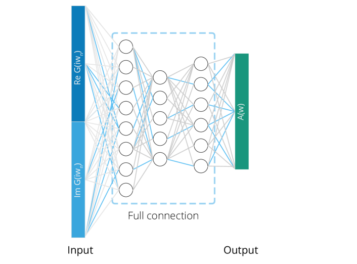
Figure 1: (Color online) FCL neural network. An illustration of our neural network architecture which consists only of FCLs. The input $G(i\omega_{n})$ is an array of complex numbers. $\Re[G(i\omega_{n})]$ and $\Im[G(i\omega_{n})]$ are arranged as a 1D array to be inserted into the neural-net input. The dropout layers are located in between all the FCLs to reduce the overfitting of neural networks (not shown). The green box represents the output layer of $A(\omega)$. The blue neural network lines are the schematic representation of activated connections.

As the first step toward ML-based analytic continuation, we consider the neural network composed of FCLs which may be regarded as an early-stage ML approach Frean (1990); Miller et al. (1990); Ripley (1994). Roughly, the use of single FCL can be regarded as one multiplication process of an inversion matrix to the input Green’s function Kung (2009). Having more FCLs thus corresponds to the increased number of matrix multiplications to represent the inversion. Practically it is not expected to achieve a notable improvement just by increasing the number of hidden layers Mühlenbein (1990); Lecun et al. (1998); Dean et al. (2012); He et al. (2016). After testing many different numbers of hidden layer sets, we indeed found that the performance is not much enhanced. Thus, in the below, we focus on the results of three layers (Fig.1).

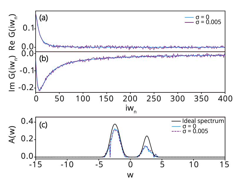
Figure 2: (Color online) Analytic continuation result of FCL. The input Green’s functions and the output spectra calculated by the FCL neural network kernel (without CNN layer). (a, b) $\Re[G(i\omega_{n})]$ and $\Im[G(i\omega_{n})]$ are presented in (a) and (b), respectively. The blue curves are generated from the ideal spectrum shown by the black line in (c). The purple lines show the noised input $G(i\omega_{n})^{\rm{in}}_{\rm{noise}}$ with $\sigma=0.005$ (see the main text for more details). (c) The calculated spectral functions are presented by blue-solid ($\sigma$=0; noise-free) and purple-dashed curve ($\sigma$=0.005) in comparison to the ideal spectrum (black-solid line).

Figure 2 presents the result of analytic continuation by using FCLs neural network. The black line in Fig. 2(c) is the spectrum from which imaginary Green’s functions of Fig. 2(a) and (b) (blue lines) are generated. Therefore, if the continuation procedure is perfect, the continued spectrum should be identical with the black line in Fig. 2(c). Note that the process of obtaining $G(i\omega_{n})$ from $A(\omega)$ is not ill-conditioned. Once $G(i\omega_{n})$ is calculated, one can perform the continuation and compare the result of $A(\omega)$ with the original one, namely the ideal spectrum.

The FCL continuation results are shown in Fig. 2(c). The blue-solid and purple-dashed line corresponds to $\sigma$=0 and $\sigma$=0.005, respectively. It is clearly noted that the continued spectra are not smooth and significantly deformed in comparison to the ideal black line. This result demonstrates the challenging nature of the problem. At the same time, however, we also note that the overall shape of spectrum is captured by our FCL neural network although the unexpected wriggles are found, and they become worse as the noise level increases. We emphasize that this level of performance is hardly achievable through the direct matrix inversion of Eq. (2). This promising aspect is largely attributed to the ‘dropout’ and the regularisation procedure which prevent overfittings Srivastava et al. (2014). In this regard, while not satisfactory at all, our FCL result shows a possibility of neural network approach for the analytic continuation.

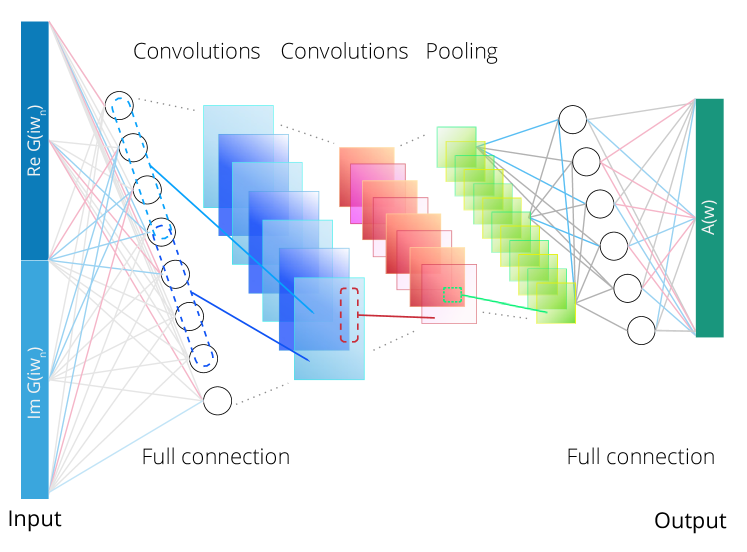
Figure 3: (Color online) CNN neural network. An illustration of the neural network architecture which consists of both FCLs and CNN. Two convolution layers (blue and red squares) and one pooling layer (green squares) are placed in between the FCLs. Coloured neural network lines are the schematic representations of activated connections.

III.2 Convolutional neural network

Many techniques have been suggested to overcome the deficiency of FCL. One key idea is to identify the essential features of a problem and to reconstruct them in a higher dimensional space Montufar et al. (2014); Pillonetto et al. (2014). Principal component analysis (PCA) Shlens (2014); Hall and Hosseini-Nasab (2006) is an example which proved to be powerful for data compression and dimensionality reduction. Unfortunately, however, PCA can only be used in rank 1 (vector) and rank 2 (matrix) for most of the cases. While some techniques for tensor PCA have been proposed, they seem to need further developments Richard and Montanari (2014); Inoue (2016); Zhang and Xia (2018); Li et al. (2015). A typical fundamental limitation of PCA is that each principal component is given by a linear combination of original variables whereas non-linearity is essential for ill-posed problems Archambeau and Bach (2009). In this regard, CNN is a useful advanced technique leading the modern machine-learning era Ciresan et al. (2011); Krizhevsky et al. (2012); Simonyan and Zisserman (2014); Szegedy et al. (2015); He et al. (2016); LeCun et al. (2015). The performance of CNN image processing surpasses the human-designed algorithms based on ‘domain knowledge’ Ciresan et al. (2011); Krizhevsky et al. (2012). Due to its outstanding feature selection in tensor space, CNN is widely adopted by high-dimensional noise filters for auto-encoder and sound/video data Masci et al. (2011); Donahue et al. (2018); Karpathy et al. (2014).

In analytic continuation, input/output data are represented by a certain set of numbers. Thus it can be regarded as an inverse problem that has to be performed within a dimension corresponding to those numbers. With this observation, we applied CNN technique to the long-standing ill-posed problem of analytic continuation. Figure 3 shows our neural network structure. We aim to create a minimal model with the smallest possible number of layers. Thus our neural network is designed to contain CNN layers in between two FCLs since we learned in the above that three FCLs could capture the basic features of spectra. While it is conventional to have CNN layers just next to the input layer in the image processing (e.g., AlexNet Krizhevsky et al. (2012), VGG Simonyan and Zisserman (2014), GoogleNet Szegedy et al. (2015), and ResNet He et al. (2016)), we take a different strategy of inserting the CNN layer after the matrix operation through FCL. It is because the full information of input Green’s function needs to be utilized in our problem. The total number of parameters in our neural network is $\sim$600,000 and $\sim$500,000 for including and excluding CNN, respectively. It is noted that the network size is not much increased by having CNN layers. We have adopted modern optimization algorithm, namely ‘Adadelta’ Zeiler (2012), to optimize this large number of neural networks parameters.

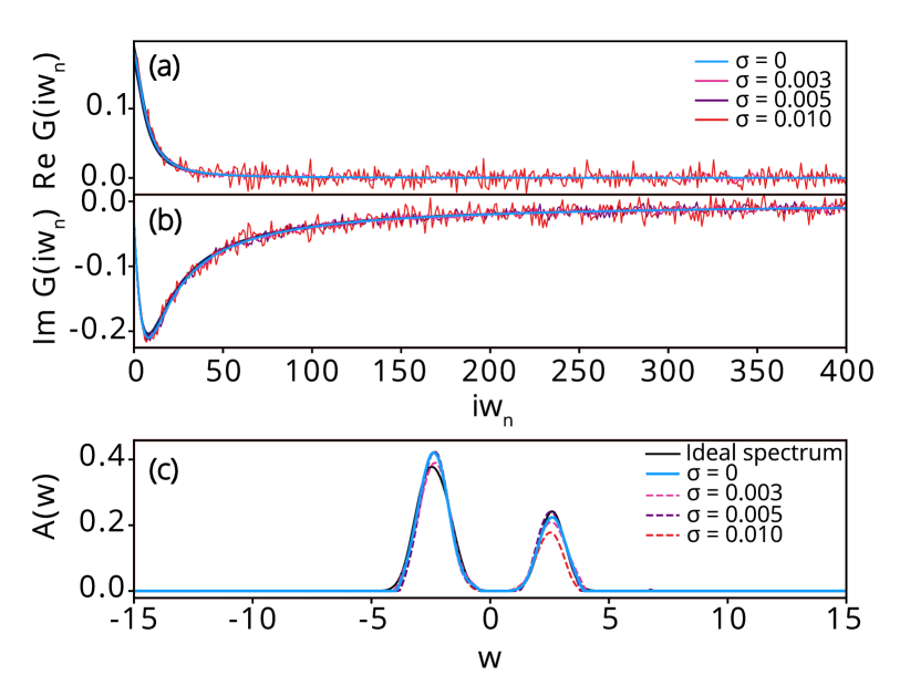
Figure 4: (Color online) Analytic continuation result of CNN. (a, b) $\Re[G(i\omega_{n})]$ and $\Im[G(i\omega_{n})]$ are presented in (a) and (b), respectively. The light-blue curves are generated from the ideal spectrum shown by the black line in (c). Five different noise levels are presented in light-blue ($\sigma$=0), magenta ($\sigma$=0.003), purple ($\sigma$=0.005) and red lines ($\sigma$=0.01). (c) Analytic continuation result of CNN-ML kernel for $\sigma$=0 (noise-free; light-blue-solid), $\sigma$=0.003 (magenta-dashed), $\sigma$=0.005 (purple-dashed) and $\sigma$=0.01 (red-dashed) along with the ideal spectrum (black-solid line).

Figure 4 shows the continuation result of using CNN. The model spectrum (black line in Fig. 4(c)) is designed to mimic a Mott-Hubbard insulator consisted of two distinct Hubbard bands with different peak heights. The outstanding performance of CNN can clearly be seen from that the continuation results are significantly improved in comparison to the FCL-only data in Fig. 2. The overall shape, peak positions and relative peak heights are well reproduced without any undesirable wriggle. Importantly, the reproducibility remains quite robust against the noise even if the deviation from the ideal spectrum (black) becomes noticeable as the noise level increases (from light-blue-solid lines to red-dashed). We also checked that the reconstructed ${\tilde{G}}(i\omega_{n})=({\rm\bf{K}}A)(i\omega_{n})$ is consistent with $G(i\omega_{n})$ within the noise level (not shown). For example, the calculated ${\tilde{\chi}}$ = 0.0044 for the case of $\sigma=0.003$ where $\tilde{\chi}\equiv(\chi^{2}/N_{\rm freq})^{-1/2}$.

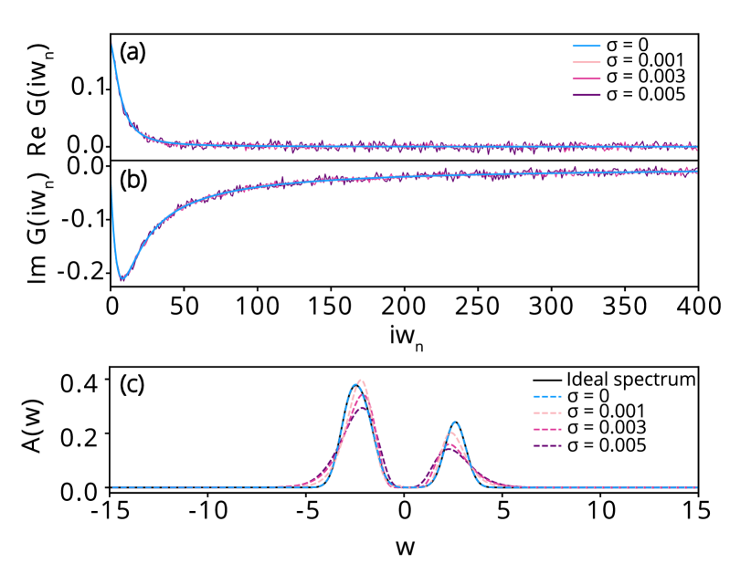
Figure 5: (Color online) Analytic continuation result of MEM. (a, b) Input Green’s function of $\Re[G(i\omega_{n})]$ and $\Im[G(i\omega_{n})]$ are presented in (a) and (b), respectively. The light blue curves are generated from the ideal spectrum shown by the black line in (c). Four different noise levels are presented in light-blue ($\sigma$=0), light-pink ($\sigma$=0.001), magenta ($\sigma$=0.003) and purple lines ($\sigma$=0.005). (c) Analytic continuation result of conventional MEM for$\sigma$=0 (noise-free; light-blue-solid), $\sigma$=0.001 (light-pink-dashed), $\sigma$=0.003 (magenta-dashed) and $\sigma$=0.005 (purple-dashed) along with the ideal spectrum (black-solid line).

The robustness against the input noise is a crucially required feature for the reliable analytic continuation since the noise is unavoidably present in stochastic approaches. As shown in Fig. 4(c), the overall features and the detailed shapes of the spectrum are well maintained even for the case of significant noise levels. This result shows the powerfulness of ML-based analytic continuation kernel.

The performance of ML kernel is further demonstrated by the comparison to the conventional continuation technique, namely MEM. The details of our MEM algorithms can be found in Ref.  Bergeron and Tremblay, 2016; Sim and Han, 2018. Fig. 5 shows the result of MEM which is one of the most widely-used methods for analytic continuation Haule et al. (2010); Bergeron and Tremblay (2016); Jarrell and Gubernatis (1996); Gunnarsson et al. (2010b). It is clearly noted that, even at a significantly lower noise level, the MEM result is markedly deviated from the ideal spectrum in terms of peak position and height. It is in a sharp contrast to the ML-based result of Fig. 4 in which the spectrum is well preserved even at $\sigma=0.01$.

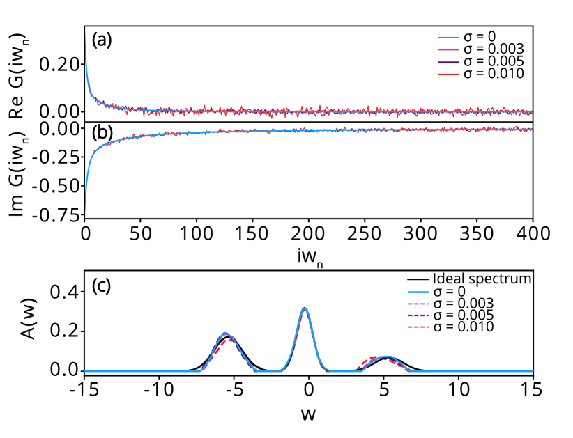
Figure 6: (Color online) Analytic continuation result of CNN for metallic spectrum. (a, b) Input Green’s function of $\Re[G(i\omega_{n})]$ and $\Im[G(i\omega_{n})]$ are presented in (a) and (b), respectively. The light-blue curves are generated from the ideal spectrum shown by the black line in (c). Five different noise levels are presented in light-blue ($\sigma$=0), magenta ($\sigma$=0.003), purple ($\sigma$=0.005) and red lines ($\sigma$=0.01). (c) Analytic continuation result of CNN-ML kernel for$\sigma$=0 (noise-free; light-blue-solid), $\sigma$=0.003 (magenta-dashed), $\sigma$=0.005 (purple-dashed) and $\sigma$=0.01 (red-dashed) along with the ideal spectrum (black-solid line).

Figure 6 shows the result of ML kernel for metallic spectrum having coherent as well as incoherent peaks. Once again, our machine-learning kernel well reproduces the original spectrum. The robustness against noise is also excellent as in the insulating case. In particular, the coherent peak is considerably well reproduced while the incoherent states are moderately affected by the noises. It is a good indication for predicting the phase from a given Green’s function.

As the last example, we present the results of a real material, namely SrVO₃ monolayer. While the bulk SrVO₃ is a correlated metal, it becomes an insulator in the monolayer limit Yoshimatsu et al. (2010); Schüler et al. (2018). The Green’s function is obtained from DFT+DMFT calculation Lichtenstein and Katsnelson (1998); Georges and Kotliar (1992) combined with the hybridization expansion continuous-time quantum Monte Carlo algorithm Werner et al. (2006); Werner and Millis (2006); Haule (2007); com . The spectra obtained by our ML kernel is reasonably well compared with those of MEM; see Fig. 7. While the peak widths are slightly narrower in MEM, it should be noted that the direct use of MEM for Green’s function tends to broaden the spectra Wang et al. (2009).

Of particular interest is the performance of our ML continuation kernel for the cases that were not included in the training sets. Although the systematic investigation of the training-set dependence is not the main interest of the current study, we obtained some meaningful results. In terms of peak numbers, the quality of continuation gets gradually worse as the number of peaks goes out of the training range. However, its performance is still quite decent (we tried up to the 25-peak case) and at least comparable with that of MEM. The similar feature is found for the peak width. For the peak of width=0.1 and 0.2, the ML kernel produces the spectrum whose width is 0.22 and 0.24, respectively. Considering that the conventional continuation techniques suffer from the same problems in describing sharp peaks, we concluded that the ML exhibits reasonably good performance. Finally, we emphasize the efficiency of ML-based analytic continuation. Once the ML kernel is well trained, the continuation process can be performed at a speed of $\sim$10,000 Green’s functions/sec, which is at least $10^{4}$–$10^{5}$ faster than the conventional MEM.

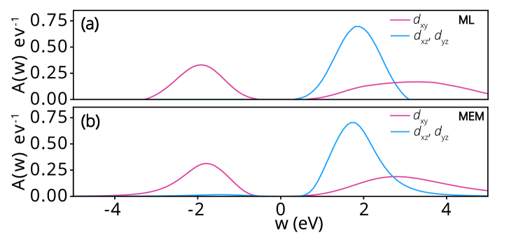
Figure 7: (Color online) The calculated DFT+DMFT spectral function of monolayer SrVO₃ by (a) CNN and (b) MEM. The magenta and blue colors refer to the $d_{xy}$ and $d_{yz,xz}$ orbital character, respectively. Comparison between ML and MEM results for DFT+DMFT spectral function of the SrVO₃ monolayer The input Green’s function is obtained from DFT+DMFT with CT-QMC solver. Analytic continuation for the spectral function was performed using (a) ML-CNN and (b) MEM.

IV Conclusion

Modern ML technique proves its usefulness for a long-standing physics problem of analytic continuation. Its superiority over the conventional technique is demonstrated in terms of the accuracy, speed, and the robustness against noise. For both insulating and metallic spectrum, our CNN-based ML kernel gives the better agreement with the ideal spectrum in terms of peak position and height. Up to the high level of random noises, at which MEM fails to produce the reliable results, ML technique retains its accuracy. In terms of computation speed, the trained kernel is 10⁴–10⁵ times faster than the conventional method. Our result suggests that ‘domain-knowledge’ free ML can be used as an alternative tool for the physics problems where the conventional methods have been struggling. We also note the possibility of certain types of hybrid methods in which a part of physics intuitions would be combined with ML approach.

V Acknowledgments

This work was supported by Basic Science Research Program through the National Research Foundation of Korea (NRF) funded by the Ministry of Education (2017R1D1A1B03032082) and Creative Materials Discovery Program through the NRF funded by Ministry of Science and ICT (2018M3D1A1059001).

References

- Vidberg and Serene (1977) H. J. Vidberg and J. W. Serene, J Low Temp Phys 29, 179 (1977).
- Gunnarsson et al. (2010a) O. Gunnarsson, M. W. Haverkort, and G. Sangiovanni, Phys. Rev. B 81 (2010a), 10.1103/PhysRevB.81.155107, arXiv:1001.4351 .
- Haule et al. (2010) K. Haule, C.-H. Yee, and K. Kim, Phys. Rev. B 81, 195107 (2010).
- Bergeron and Tremblay (2016) D. Bergeron and A.-M. S. Tremblay, Phys. Rev. E 94, 023303 (2016).
- Jarrell and Gubernatis (1996) M. Jarrell and J. E. Gubernatis, Physics Reports 269, 133 (1996).
- Gunnarsson et al. (2010b) O. Gunnarsson, M. W. Haverkort, and G. Sangiovanni, Phys. Rev. B 82, 165125 (2010b).
- Sandvik (1998) A. W. Sandvik, Phys. Rev. B 57, 10287 (1998).
- Rifai et al. (2011) S. Rifai, Y. N. Dauphin, P. Vincent, Y. Bengio, and X. Muller, in Advances in Neural Information Processing Systems (2011) pp. 2294–2302.
- Goodfellow et al. (2016) I. Goodfellow, Y. Bengio, and A. Courville, Deep Learning (The MIT Press, Cambridge, Massachusetts, 2016).
- Zhu et al. (2016) F. Zhu, L. Shao, J. Xie, and Y. Fang, Image and Vision Computing Handcrafted vs. Learned Representations for Human Action Recognition, 55, 42 (2016).
- LeCun et al. (2015) Y. LeCun, Y. Bengio, and G. Hinton, Nature 521, 436 (2015).
- Silver et al. (2016) D. Silver, A. Huang, C. J. Maddison, A. Guez, L. Sifre, G. van den Driessche, J. Schrittwieser, I. Antonoglou, V. Panneershelvam, M. Lanctot, S. Dieleman, D. Grewe, J. Nham, N. Kalchbrenner, I. Sutskever, T. Lillicrap, M. Leach, K. Kavukcuoglu, T. Graepel, and D. Hassabis, Nature 529, 484 (2016).
- Behler and Parrinello (2007) J. Behler and M. Parrinello, Phys. Rev. Lett. 98, 146401 (2007).
- Faber et al. (2016) F. A. Faber, A. Lindmaa, O. A. von Lilienfeld, and R. Armiento, Phys. Rev. Lett. 117, 135502 (2016).
- Seko et al. (2017) A. Seko, H. Hayashi, K. Nakayama, A. Takahashi, and I. Tanaka, Phys. Rev. B 95 (2017), 10.1103/PhysRevB.95.144110, arXiv:1611.08645 .
- Kolb et al. (2017) B. Kolb, L. C. Lentz, and A. M. Kolpak, Scientific Reports 7, 1192 (2017).
- Behler (2016) J. Behler, The Journal of Chemical Physics 145, 170901 (2016).
- Artrith et al. (2017) N. Artrith, A. Urban, and G. Ceder, Phys. Rev. B 96, 014112 (2017).
- Torlai and Melko (2016) G. Torlai and R. G. Melko, Phys. Rev. B 94 (2016), arXiv: 1606.02718.
- Huang and Wang (2017) L. Huang and L. Wang, Phys. Rev. B 95, 035105 (2017).
- Carrasquilla and Melko (2017) J. Carrasquilla and R. G. Melko, Nat Phys 13, 431 (2017).
- Arsenault et al. (2014) L.-F. Arsenault, A. Lopez-Bezanilla, O. A. von Lilienfeld, and A. J. Millis, Phys. Rev. B 90 (2014), 10.1103/PhysRevB.90.155136, arXiv:1408.1143 .
- Li et al. (2016) L. Li, T. E. Baker, S. R. White, and K. Burke, Phys. Rev. B 94 (2016).
- Wang (2016) L. Wang, Phys. Rev. B 94, 195105 (2016).
- Carleo and Troyer (2017) G. Carleo and M. Troyer, Science 355, 602 (2017).
- Ch’ng et al. (2017) K. Ch’ng, J. Carrasquilla, R. G. Melko, and E. Khatami, Phys. Rev. X 7 (2017), arXiv: 1609.02552.
- Wang et al. (2017) J. Wang, S. Paesani, R. Santagati, S. Knauer, A. A. Gentile, N. Wiebe, M. Petruzzella, J. L. O’Brien, J. G. Rarity, A. Laing, and M. G. Thompson, Nat Phys 13, 551 (2017).
- Zhang and Kim (2017) Y. Zhang and E.-A. Kim, Phys. Rev. Lett. 118, 216401 (2017).
- Cai et al. (2015) X.-D. Cai, D. Wu, Z.-E. Su, M.-C. Chen, X.-L. Wang, L. Li, N.-L. Liu, C.-Y. Lu, and J.-W. Pan, Phys. Rev. Lett. 114, 110504 (2015).
- Dunjko et al. (2016) V. Dunjko, J. M. Taylor, and H. J. Briegel, Phys. Rev. Lett. 117, 130501 (2016).
- Lau et al. (2017) H.-K. Lau, R. Pooser, G. Siopsis, and C. Weedbrook, Phys. Rev. Lett. 118, 080501 (2017).
- Torlai and Melko (2017) G. Torlai and R. G. Melko, Phys. Rev. Lett. 119, 030501 (2017).
- Tubiana and Monasson (2017) J. Tubiana and R. Monasson, Phys. Rev. Lett. 118, 138301 (2017), arXiv:1611.06759 .
- Bengio et al. (2007) Y. Bengio, P. Lamblin, D. Popovici, and H. Larochelle, in Advances in Neural Information Processing Systems 19, edited by B. Schölkopf, J. C. Platt, and T. Hoffman (2007) pp. 153–160.
- Montufar et al. (2014) G. F. Montufar, R. Pascanu, K. Cho, and Y. Bengio, in Advances in Neural Information Processing Systems 27, edited by Z. Ghahramani, M. Welling, C. Cortes, N. D. Lawrence, and K. Q. Weinberger (2014) pp. 2924–2932.
- Kalchbrenner et al. (2014) N. Kalchbrenner, E. Grefenstette, and P. Blunsom, in Proceedings of the 52nd Annual Meeting of the Association for Computational Linguistics (Volume 1: Long Papers) (Association for Computational Linguistics, Baltimore, Maryland, 2014) pp. 655–665.
- Zeiler (2012) M. D. Zeiler, ArXiv12125701 Cs (2012), arXiv:1212.5701 [cs] .
- Kingma and Ba (2014) D. P. Kingma and J. Ba, ArXiv14126980 Cs (2014), arXiv:1412.6980 [cs] .
- Duchi et al. (2011) J. Duchi, E. Hazan, and Y. Singer, J Mach Learn Res 12, 2121 (2011).
- Arsenault et al. (2017) L.-F. Arsenault, R. Neuberg, L. A. Hannah, and A. J. Millis, Inverse Probl. 33, 115007 (2017).
- Lecun et al. (1998) Y. Lecun, L. Bottou, Y. Bengio, and P. Haffner, Proc. IEEE 86, 2278 (1998).
- Vapnik (1999) V. N. Vapnik, IEEE Trans. Neural Netw. 10, 988 (1999).
- Pillonetto et al. (2014) G. Pillonetto, F. Dinuzzo, T. Chen, G. De Nicolao, and L. Ljung, Automatica 50, 657 (2014).
- Krizhevsky et al. (2012) A. Krizhevsky, I. Sutskever, and G. E. Hinton, in Advances in Neural Information Processing Systems 25, edited by F. Pereira, C. J. C. Burges, L. Bottou, and K. Q. Weinberger (2012) pp. 1097–1105.
- Farabet et al. (2013) C. Farabet, C. Couprie, L. Najman, and Y. LeCun, IEEE Trans. Pattern Anal. Mach. Intell. 35, 1915 (2013).
- Szegedy et al. (2015) C. Szegedy, W. Liu, Y. Jia, P. Sermanet, S. Reed, D. Anguelov, D. Erhan, V. Vanhoucke, and A. Rabinovich, in 2015 IEEE Conference on Computer Vision and Pattern Recognition (CVPR) (2015) pp. 1–9.
- Tompson et al. (2014) J. J. Tompson, A. Jain, Y. LeCun, and C. Bregler, in Advances in Neural Information Processing Systems 27, edited by Z. Ghahramani, M. Welling, C. Cortes, N. D. Lawrence, and K. Q. Weinberger (2014) pp. 1799–1807.
- Mikolov et al. (2011) T. Mikolov, A. Deoras, D. Povey, L. Burget, and J. Černocký, in 2011 IEEE Workshop on Automatic Speech Recognition Understanding (2011) pp. 196–201.
- Hinton et al. (2012) G. Hinton, L. Deng, D. Yu, G. E. Dahl, A. Mohamed, N. Jaitly, A. Senior, V. Vanhoucke, P. Nguyen, T. N. Sainath, and B. Kingsbury, IEEE Signal Process. Mag. 29, 82 (2012).
- Sainath et al. (2013) T. N. Sainath, A. Mohamed, B. Kingsbury, and B. Ramabhadran, in 2013 IEEE International Conference on Acoustics, Speech and Signal Processing (2013) pp. 8614–8618.
- Collobert et al. (2011) R. Collobert, J. Weston, L. Bottou, M. Karlen, K. Kavukcuoglu, and P. Kuksa, J Mach Learn Res 12, 2493 (2011).
- Cho et al. (2014) K. Cho, B. van Merrienboer, C. Gulcehre, D. Bahdanau, F. Bougares, H. Schwenk, and Y. Bengio, in Proceedings of the 2014 Conference on Empirical Methods in Natural Language Processing (EMNLP) (Association for Computational Linguistics, Doha, Qatar, 2014) pp. 1724–1734.
- Jean et al. (2014) S. Jean, K. Cho, R. Memisevic, and Y. Bengio, ArXiv14122007 Cs (2014), arXiv:1412.2007 [cs] .
- Sutskever et al. (2014) I. Sutskever, O. Vinyals, and Q. V. V. Le, in Advances in Neural Information Processing Systems 27, edited by Z. Ghahramani, M. Welling, C. Cortes, N. D. Lawrence, and K. Q. Weinberger (2014) pp. 3104–3112.
- Ciresan et al. (2011) D. C. Ciresan, U. Meier, L. M. Gambardella, and J. Schmidhuber, in 2011 International Conference on Document Analysis and Recognition (2011) pp. 1135–1139.
- Simonyan and Zisserman (2014) K. Simonyan and A. Zisserman, ArXiv14091556 Cs (2014), arXiv:1409.1556 [cs] .
- He et al. (2016) K. He, X. Zhang, S. Ren, and J. Sun, in 2016 IEEE Conference on Computer Vision and Pattern Recognition (CVPR) (2016) pp. 770–778.
- Masci et al. (2011) J. Masci, U. Meier, D. Cireşan, and J. Schmidhuber, in Artificial Neural Networks and Machine Learning – ICANN 2011, Lecture Notes in Computer Science (Springer, Berlin, Heidelberg, 2011) pp. 52–59.
- Donahue et al. (2018) C. Donahue, J. McAuley, and M. Puckette, ArXiv180204208 Cs (2018), arXiv:1802.04208 [cs] .
- Karpathy et al. (2014) A. Karpathy, G. Toderici, S. Shetty, T. Leung, R. Sukthankar, and L. Fei-Fei, in Proceedings of the IEEE Conference on Computer Vision and Pattern Recognition (2014) pp. 1725–1732.
- Chollet et al. (2015) F. Chollet et al., “Keras,” https://github.com/keras-team/keras (2015).
- Abadi et al. (2015) M. Abadi, A. Agarwal, P. Barham, E. Brevdo, Z. Chen, C. Citro, G. S. Corrado, A. Davis, J. Dean, M. Devin, S. Ghemawat, I. Goodfellow, A. Harp, G. Irving, M. Isard, Y. Jia, R. Jozefowicz, L. Kaiser, M. Kudlur, J. Levenberg, D. Mané, R. Monga, S. Moore, D. Murray, C. Olah, M. Schuster, J. Shlens, B. Steiner, I. Sutskever, K. Talwar, P. Tucker, V. Vanhoucke, V. Vasudevan, F. Viégas, O. Vinyals, P. Warden, M. Wattenberg, M. Wicke, Y. Yu, and X. Zheng, “TensorFlow: Large-scale machine learning on heterogeneous systems,” (2015), software available from tensorflow.org.
- Tieleman and Hinton (2012) T. Tieleman and G. Hinton, COURSERA Neural Netw. Mach. Learn. 4, 26 (2012).
- Hahnloser et al. (2000) R. H. Hahnloser, R. Sarpeshkar, M. A. Mahowald, R. J. Douglas, and H. S. Seung, Nature 405, 947 (2000).
- Ramachandran et al. (2017) P. Ramachandran, B. Zoph, and Q. V. Le, ArXiv171005941 Cs (2017), arXiv:1710.05941 [cs] .
- Klambauer et al. (2017) G. Klambauer, T. Unterthiner, A. Mayr, and S. Hochreiter, in Advances in Neural Information Processing Systems 30, edited by I. Guyon, U. V. Luxburg, S. Bengio, H. Wallach, R. Fergus, S. Vishwanathan, and R. Garnett (2017) pp. 971–980.
- Frean (1990) M. Frean, Neural Comput. 2, 198 (1990).
- Miller et al. (1990) W. T. Miller, R. P. Hewes, F. H. Glanz, and L. G. Kraft, IEEE Trans. Robot. Autom. 6, 1 (1990).
- Ripley (1994) B. D. Ripley, J. R. Stat. Soc. Ser. B Methodol. 56, 409 (1994).
- Kung (2009) S.-Y. Kung, in Advances in Multimedia Information Processing - PCM 2009, edited by P. Muneesawang, F. Wu, I. Kumazawa, A. Roeksabutr, M. Liao, and X. Tang (Springer Berlin Heidelberg, Berlin, Heidelberg, 2009) pp. 1–32.
- Mühlenbein (1990) H. Mühlenbein, Parallel Comput. 14, 249 (1990).
- Dean et al. (2012) J. Dean, G. Corrado, R. Monga, K. Chen, M. Devin, M. Mao, M. Ranzato, A. Senior, P. Tucker, K. Yang, Q. V. Le, and A. Y. Ng, in Advances in Neural Information Processing Systems 25, edited by F. Pereira, C. J. C. Burges, L. Bottou, and K. Q. Weinberger (2012) pp. 1223–1231.
- Srivastava et al. (2014) N. Srivastava, G. Hinton, A. Krizhevsky, I. Sutskever, and R. Salakhutdinov, J. Mach. Learn. Res. 15, 1929 (2014).
- Shlens (2014) J. Shlens, ArXiv14041100 Cs Stat (2014), arXiv:1404.1100 [cs, stat] .
- Hall and Hosseini-Nasab (2006) P. Hall and M. Hosseini-Nasab, J. R. Stat. Soc. Ser. B Stat. Methodol. 68, 109 (2006).
- Richard and Montanari (2014) E. Richard and A. Montanari, in Advances in Neural Information Processing Systems 27, edited by Z. Ghahramani, M. Welling, C. Cortes, N. D. Lawrence, and K. Q. Weinberger (2014) pp. 2897–2905.
- Inoue (2016) K. Inoue, in Applied Matrix and Tensor Variate Data Analysis, edited by T. Sakata (Springer Japan, Tokyo, 2016) pp. 51–71.
- Zhang and Xia (2018) A. Zhang and D. Xia, IEEE Trans. Inf. Theory 64, 7311 (2018).
- Li et al. (2015) H. Li, Z. Lin, X. Shen, J. Brandt, and G. Hua, in Proceedings of the IEEE Conference on Computer Vision and Pattern Recognition (2015) pp. 5325–5334.
- Archambeau and Bach (2009) C. Archambeau and F. R. Bach, in Advances in Neural Information Processing Systems 21, edited by D. Koller, D. Schuurmans, Y. Bengio, and L. Bottou (2009) pp. 73–80.
- Sim and Han (2018) J.-H. Sim and M. J. Han, Phys. Rev. B 98, 205102 (2018).
- Yoshimatsu et al. (2010) K. Yoshimatsu, T. Okabe, H. Kumigashira, S. Okamoto, S. Aizaki, A. Fujimori, and M. Oshima, Phys. Rev. Lett. 104, 147601 (2010).
- Schüler et al. (2018) M. Schüler, O. E. Peil, G. J. Kraberger, R. Pordzik, M. Marsman, G. Kresse, T. O. Wehling, and M. Aichhorn, J. Phys.: Condens. Matter 30, 475901 (2018).
- Lichtenstein and Katsnelson (1998) A. I. Lichtenstein and M. I. Katsnelson, Phys. Rev. B 57, 6884 (1998).
- Georges and Kotliar (1992) A. Georges and G. Kotliar, Phys. Rev. B 45, 6479 (1992).
- Werner et al. (2006) P. Werner, A. Comanac, L. de’ Medici, M. Troyer, and A. J. Millis, Phys. Rev. Lett. 97, 076405 (2006).
- Werner and Millis (2006) P. Werner and A. J. Millis, Phys. Rev. B 74, 155107 (2006).
- Haule (2007) K. Haule, Phys. Rev. B 75, 155113 (2007).
- (89) The optimized lattice structure of Ref. Schüler et al., 2018 was used for DFT+DMFT calculation and we adopted -points. Atomic V- orbitals are constructed from Maximally localized Wannier functions Marzari and Vanderbilt (1997); Souza et al. (2001); ope . The Slater-Kanamori interaction parameters are eV and eV Schüler et al. (2018); Bhandary et al. (2016).
- Wang et al. (2009) X. Wang, E. Gull, L. de’ Medici, M. Capone, and A. J. Millis, Phys. Rev. B 80, 045101 (2009).
- Marzari and Vanderbilt (1997) N. Marzari and D. Vanderbilt, Phys Rev B 56, 12847 (1997).
- Souza et al. (2001) I. Souza, N. Marzari, and D. Vanderbilt, Phys Rev B 65, 035109 (2001).
- (93) http://www.openmx-square.org.
- Bhandary et al. (2016) S. Bhandary, E. Assmann, M. Aichhorn, and K. Held, Phys. Rev. B 94, 155131 (2016).