Chained Einstein-Podolsky-Rosen steering inequalities with improved visibility

Abstract

It is known that the linear $n$-setting steering inequalities introduced in Ref. [Nature Phys. 6, 845 (2010)] are very efficient inequalities in detecting steerability of the Werner states by using optimal measurement axes. Here, we construct chained steering inequalities that have improved visibility for the Werner states under a finite number of settings. Specifically, the threshold values of quantum violation of our inequalities for the $n=4,6,10$ settings are lower than those of the linear steering inequalities. Furthermore, for almost all generalized Werner states, the chained steering inequalities always have improved visibility in comparison with the linear steering inequalities.

I Introduction

Entanglement is a property of distributed quantum systems that has no classical counterpart and challenges our everyday-life intuition about the physical world Horodecki . It is the key element in many quantum information processing tasks Nielsen . The origin of steering, a notion closely related with entanglement, can historically be traced back to Schr$\rm{\ddot{o}}$dinger’s reply Schrodinger to the well-known Einstein-Podolsky-Rosen (EPR) argument epr35 . However, steering lacked operational meanings, until the year 2007 when it was given a rigorous definition through the quantum information task Wiseman . Then it becomes clearer that the EPR paradox concerns more precisely the existence of local hidden state (LHS) models, rather than that of local hidden variable (LHV) models Bell ; epr35 ; gisin91 ; wernerJPA . After 2007, EPR steering has gained a very rapid development in theory Chen ; Skrzypczyk ; Bowles ; chenSR ; chenRC ; Cavalcanti and experiment wisemanNature ; Sun . Different from entanglement and Bell nonlocality Brunner , steering possesses a curious feature of “one-way quantumness” Bowles , which is shown useful in one-way quantum information tasks like, e.g., one-way quantum cryptography one-way-steer .

Intriguingly, the authors of Wiseman proved that steerable states are a strict subset of the entangled states, and a strict superset of the states that can exhibit Bell nonlocality. In analogy to the violation of Bell’s inequality which implies Bell nonlocality, any violation of a steering inequality immediately implies EPR steering chenRC ; wisemanNature . It is in principle easier to experimentally observe the violation than Bell inequalities, because one has no concerns about closing the notorious locality loophole as in a Bell test Brunner .

Among many others, the $n$-setting linear steering inequalities in wisemanNature have been experimentally verified by the violation with the Werner states in their optimal measurement axes. In this paper, comparing with those in wisemanNature , we focus on the generalized Werner states and address the question of whether there exist steering inequalities that have improved visibility so that steering is more robust against white noise and thus more experiment-friendly to test in practice. Below, in the Alice-to-Bob steering scenario, we shall construct chained steering inequalities out of the chained Bell inequalities, and demonstrate that with Bob’s measurement directions properly adjusted, one can obtain lower threshold values above which these inequalities can be violated.

The paper is structured as follows. In Sec. II, we shall briefly review two family of $n$-setting steering inequalities: the linear wisemanNature and the chained Meng , along with threshold values of their violation. In Sec. III, we will present new measure directions, obtain new chained steering inequalities, and then compute the threshold values for the obtained chained inequalities, which are shown to be lower than those of the linear inequalities. In Sec. IV, focus on the generalized Werner states, we research the region of their parameters that can have the inequalities violated, and find that for almost all generalized Werner states the new chained steering inequalities always have improved visibility in comparison with the linear steering inequalities. We discuss the results in Sec. V.

II Two known families of steering inequalities

In this section, we first review two families of steering inequalities, and then give the threshold values of their violation.

II.1 The $n$-setting linear steering inequalities

For qubit systems, we can take Bob’s $i$-th measurement as the Pauli observable $\hat{\sigma}_{i}^{B}$ along some axis $b[i]$. By denoting Alice’s declared result(we make no assumption that it is derived from a quantum measurement) as random variables $A_{i}\in\{1,-1\}$ for all $i$, the $n$-setting linear steering inequality is of the form

$$I_{n}\equiv\frac{1}{n}\sum_{i=1}^{n}\langle A_{i}\hat{\sigma}_{i}^{B}\rangle\overset{\rm LHS}{\leq}C_{n}.$$ (1)

The LHS bound $C_{n}$ is the maximum value that $I_{n}$ can reach if Bob has a pre-existing state known to Alice, rather than half of an entangled pair shared with Alice. Clearly, the quantum bound of $I_{n}$ is just $1$. In general, for a given set of Bob’s directions

$$b[i]=\left(\sin\theta_{b_{i}}\cos\phi_{b_{i}},\sin\theta_{b_{i}}\sin\phi_{b_{i}},\cos\theta_{b_{i}}\right),$$ (2)

one has then

$$\hat{\sigma}_{i}^{B}=\sin\theta_{b_{i}}\cos\phi_{b_{i}}\sigma_{x}+\sin\theta_{b_{i}}\sin\phi_{b_{i}}\sigma_{y}+\cos\theta_{b_{i}}\sigma_{z},$$

where $\sigma_{x},\sigma_{y},\sigma_{z}$ are the Pauli matrices. If the directions are chosen as along the vertices of Platonic solids, as in Figure 2 of Ref. wisemanNature , the analytical expressions for the bounds read

$$C_{2}=\frac{1}{\sqrt{2}}\approx 0.707107,$$ (3)

$$C_{3}=C_{4}=\frac{1}{\sqrt{3}}\approx 0.57735,$$

$$C_{6}=1-\frac{5}{3\sqrt{10+2\sqrt{5}}}\sqrt{4-\sec^{2}{\frac{3\pi}{10}}}$$

$$~{}~{}~{}=\frac{1+\sqrt{5}}{6}\approx 0.539345,$$

$$C_{10}=1-\frac{1}{10}\left(1+\frac{\tan{\frac{2\pi}{5}}}{\sin{\frac{\pi}{5}}}\right)\sqrt{\frac{24}{3+\sqrt{5}}-4}$$

$$~{}~{}~{}=\frac{3+\sqrt{5}}{10}\approx 0.523607.$$

II.2 The $n$-setting chained steering inequalities

The chained steering inequality for a given $n$ is of the form Meng

$$\mathcal{I}_{n}\overset{{\rm LHS}}{\leq}\mathcal{C}_{n},$$ (4)

where

$$\mathcal{I}_{n}=\langle A_{1}\hat{\sigma}_{1}^{B}\rangle+\langle A_{2}\hat{\sigma}_{1}^{B}\rangle+\langle A_{2}\hat{\sigma}_{2}^{B}\rangle+$$ (5)

$$~{}~{}~{}~{}~{}~{}~{}~{}~{}~{}~{}\langle A_{3}\hat{\sigma}_{2}^{B}\rangle+\langle A_{3}\hat{\sigma}_{3}^{B}\rangle+\langle A_{4}\hat{\sigma}_{3}^{B}\rangle+\cdots+$$

$$~{}~{}~{}~{}~{}~{}~{}~{}~{}~{}~{}\langle A_{n}\hat{\sigma}_{n}^{B}\rangle-\langle A_{1}\hat{\sigma}_{n}^{B}\rangle,$$

and $\mathcal{C}_{n}$ is the bound for LHS models. For each $n$, if Bob chooses his measurement directions as

$$b[i]=\left(\sin{\frac{(2i-1)\pi}{2n}},0,\cos{\frac{(2i-1)\pi}{2n}}\right),$$ (6)

with $i=1,2,\cdots,n$, then the LHS bound equals Meng

$$\mathcal{C}_{n}=2\cot{\frac{\pi}{2n}},$$ (7)

which is attained at $A_{1}=A_{2}=\cdots=A_{n}=1.$

II.3 Threshold value of quantum violation

For a given set of Alice’s measurement directions

$$a[i]=\left(\sin\theta_{a_{i}}\cos\phi_{a_{i}},\sin\theta_{a_{i}}\sin\phi_{a_{i}},\cos\theta_{a_{i}}\right),$$ (8)

the observables that Alice uses read

$$A_{i}=\sin\theta_{a_{i}}\cos\phi_{a_{i}}\sigma_{x}+\sin\theta_{a_{i}}\sin\phi_{a_{i}}\sigma_{y}+\cos\theta_{a_{i}}\sigma_{z}.$$

The quantum violation, $\mathcal{Q}_{n}$, can then be obtained by numerating all possible $a[i]$.

Let us consider the Werner state

$$\rho=V|\psi\rangle\langle\psi|+(1-V)\frac{I_{4}}{4},$$ (9)

where $|\psi\rangle$ denotes the maximally entangled state

$$|\psi\rangle=\frac{1}{\sqrt{2}}(|0\rangle\otimes|1\rangle-|1\rangle\otimes|0\rangle),$$ (10)

$|0\rangle$ and $|1\rangle$ are eigenstates of $\sigma_{z}$ with eigenvalues 1 and $-1$, respectively, and $I_{4}$ is the identity matrix on $\mathbb{C}^{2}\otimes\mathbb{C}^{2}$. Let us define the visibility as

$$\mathcal{V}_{n}={\mathcal{C}_{n}}/{\mathcal{Q}_{n}}.$$ (11)

For each $n$-measurement setting, the quantity $\mathcal{V}_{n}$ describes the threshold value, above which the state (9) cannot be described by LHS models.

Remark 1.—The visibility for inequality (1), defined similarly as

$${V}_{n}={{C}_{n}}/{{Q}_{n}}={{C}_{n}}/{1}={C}_{n},$$ (12)

equals $V$ for all $n$. Namely, inequality (1) can only detect by its violation the steerability of Werner states with $V>C_{n}$.

Remark 2.—For Bob’s directions (6), the maximum quantum violation is computed as Meng

$$\mathcal{Q}_{n}=2n\cos{\frac{\pi}{2n}},$$ (13)

and so from (7) and (11) the visibility for (4) equals

$$\mathcal{V}_{n}=\frac{1}{n\sin{\frac{\pi}{2n}}}.$$ (14)

The directions (6) are not optimal for inequality (4), as there exist other directions to obtain a lower visibility. In the following section, we will present new measurement directions, obtain new chained steering inequality. Moreover, we compute threshold values for these new chained steering equalities and compare them with ones for the $n$-setting linear steering inequalities and (14).

III Chained Steering Inequalities with improved visibility

III.1 A simple example: $n=4$

When Bob chooses

$$\begin{split}&\theta_{b_{1}}=\frac{5\pi}{4},~{}\phi_{b_{1}}=\frac{\pi}{3},~{}\theta_{b_{2}}=0,~{}\phi_{b_{2}}=\frac{11\pi}{6},\\ &\theta_{b_{3}}=\frac{3\pi}{5},~{}\phi_{b_{3}}=\frac{3\pi}{4},~{}\theta_{b_{4}}=\frac{3\pi}{2},~{}\phi_{b_{4}}=\frac{\pi}{2},\end{split}$$ (15)

i.e.,

$$\begin{split}&b[1]=\left(-\frac{\sqrt{2}}{4},-\frac{\sqrt{6}}{4},-\frac{\sqrt{2}}{2}\right),\\ &b[2]=\biggr{(}0,0,1\biggr{)},\\ &b[3]=\left(-\frac{\sqrt{5+\sqrt{5}}}{4},\frac{\sqrt{5+\sqrt{5}}}{4},\frac{1-\sqrt{5}}{4}\right),\\ &b[4]=\biggr{(}0,-1,0\biggr{)},\end{split}$$ (16)

one can have

$$\begin{split}&\mathcal{Q}_{4}\approx 3.630746,~{}~{}\mathcal{C}_{4}\approx 2.055877,~{}~{}\mathcal{V}_{4}\approx 0.566241.\end{split}$$ (17)

Here, the visibility is lower than that of the linear steering inequality, for which ${V}_{4}=C_{4}\approx 0.57735$. This example implies that there exists new chained steering inequality such that its visibility lower than that of (1). We shall find new chained steering inequalities with lower threshold values numerically and list the results below.

III.2 The lowest threshold values: $n=2,3,4,6,10$

We now list Bob’s measurement directions satisfying that for these directions the new chained steering inequalities have the lowest threshold values compared with the $n$-setting linear steering inequality and the chained steering inequalities in Meng .

• $n=2$: For arbitrary directions that Bob chooses, we always have

  $$\mathcal{V}_{2}=\frac{1}{\sqrt{2}}\approx 0.707107.$$ (18)

• $n=3$: If Bob chooses the directions (6), then

  $$\mathcal{Q}_{3}=3\sqrt{3},~{}~{}~{}\mathcal{C}_{3}=2\sqrt{3},$$ (19)

  and so

  $$\mathcal{V}_{3}=\frac{2}{3}\approx 0.666667.$$ (20)

  In fact, this is the minimal threshold value, which can be confirmed by running all possible directions numerically. What is worth noting is that to get this value Bob’s directions are not unique. For instance, if Bob chooses instead the following

  $$\begin{split}b[1]=(0,0,1),\\ b[2]=(1,0,0),\\ b[3]=(0,1,0),\end{split}$$ (21)

  i.e.,

  $$\begin{split}&\theta_{1}=0,~{}~{}\phi_{1}=0,~{}~{}\theta_{2}=\frac{\pi}{2},\\ &\phi_{2}=0,~{}~{}\theta_{3}=\frac{\pi}{2},~{}~{}\phi_{3}=\frac{\pi}{2},\end{split}$$ (22)

  which is the same to what Bob chooses in the Figure 2 of Ref. wisemanNature , then, again,

  $$\mathcal{Q}_{3}=3\sqrt{2},~{}~{}\mathcal{C}_{3}=2\sqrt{2},~{}~{}\mathcal{V}_{3}=\frac{2}{3}.$$ (23)

• $n=4$: Bob chooses

  $$\begin{split}b[1]&=(0.387712,0.325511,0.862393),\\ b[2]&=(0.662244,0.014395,-0.74915),\\ b[3]&=(-0.393555,-0.764746,0.510174),\\ b[4]&=(0.256293,0.92029,0.295602),\end{split}$$ (24)

  such that

  $$\begin{split}&\mathcal{Q}_{4}\approx 3.605552,~{}~{}\mathcal{C}_{4}=2,~{}~{}\mathcal{V}_{4}\approx 0.5547.\end{split}$$ (25)

• $n=6$: Bob chooses

  $$\begin{split}b[1]&=(-0.40343,-0.594926,-0.695203),\\ b[2]&=(0.786331,-0.613429,0.073405),\\ b[3]&=(0.39261,0.6444655,0.656141),\\ b[4]&=(-0.445744,-0.539581,0.714258),\\ b[5]&=(0.795316,-0.595208,0.114891),\\ b[6]&=(0.435205,0.494333,-0.752484),\end{split}$$ (26)

  such that

  $$\begin{split}&\mathcal{Q}_{6}\approx 8.387765,~{}~{}~{}\mathcal{C}_{6}\approx 4.426295,\\ &~{}~{}\mathcal{V}_{6}\approx 0.527709.\end{split}$$ (27)

• $n=10$: Bob chooses

  $$\begin{split}b[1]&=(-0.236305,-0.475636,0.847308),\\ b[2]&=(-0.858832,0.00901434,0.512178),\\ b[3]&=(0.320136,0.687104,0.652228),\\ b[4]&=(-0.137947,0.990267,-0.0185065),\\ b[5]&=(0.774103,0.422827,-0.47115),\\ b[6]&=(0.637737,0.18577,0.747517),\\ b[7]&=(0.0326946,0.0548708,0.997958),\\ b[8]&=(0.829632,-0.326344,-0.453001),\\ b[9]&=(0.723801,-0.672939,0.152531),\\ b[10]&=(-0.296751,-0.478204,0.826595),\end{split}$$ (28)

  such that

  $$\begin{split}&\mathcal{Q}_{10}\approx 14.702807,~{}~{}~{}\mathcal{C}_{10}\approx 7.615109,\\ &~{}~{}\mathcal{V}_{10}\approx 0.517936.\end{split}$$ (29)

A comparison between the results on the linear inequalities (1), on the chained steering inequalities in Meng , and the new chained steering inequalities is listed in Table 1.

Table 1: Comparison of the visibility of inequality (1), inequalities in Meng , and the new chained inequalities.

$V_{n},~{}\mathcal{V}_{n}$	$n=2$	$n=3$	$n=4$	$n=6$	$n=10$
Inequality (1)	$\frac{1}{\sqrt{2}}$	$\frac{1}{\sqrt{3}}$	$\frac{1}{\sqrt{3}}$	$\frac{1+\sqrt{5}}{6}$	$\frac{3+\sqrt{5}}{10}$
Inequality in Meng	$\frac{1}{\sqrt{2}}$	$\frac{2}{3}$	$\frac{1}{4\sin{\frac{\pi}{8}}}$	$\frac{1}{6\sin{\frac{\pi}{12}}}$	$\frac{1}{10\sin{\frac{\pi}{20}}}$
The new inequality	$\frac{1}{\sqrt{2}}$	$\frac{2}{3}$	$0.5547$	$0.527709$	$0.517936$

We also plot the relationship between $\mathcal{V}_{n}$ and $n$ for (1), the chained steering inequalities in  Meng , and the new chained steering inequalities in Fig. 1. We can see that the new chained inequality has the lowest visibility for $n=4,6,10$.

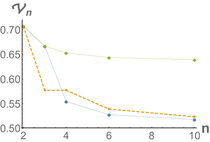
Figure 1: The relationship between the minimal $\mathcal{V}_{n}$ and $n$ for the inequality (1), inequalities in Meng , and the new chained inequalities. The yellow dashed lines, the green solid lines and the blue solid lines are for (1), inequalities in Meng , and the new chained inequalities, respectively.

IV Visibility of quantum violation with the generalized Werner states

Now we investigate the visibility for the generalized Werner states

$$\varrho=V|\psi(\theta)\rangle\langle\psi(\theta)|+(1-V)\frac{I_{4}}{4},$$ (30)

where

$$|\psi(\theta)\rangle=\cos{\theta}|00\rangle+\sin{\theta}|11\rangle.$$ (31)

Let Bob choose directions along the vertices of Platonic solids (as in Figure 2 of wisemanNature ) for (1), and directions (24), (26) and (28) for (4), then one can find their corresponding threshold values of violation.

The results are summarized in Table 2 and Fig. 2. Before ending this section, we have a few observations.

Observation 1.—The smallest threshold value is attained at $\theta=\pi/4$, reducing to the results in previous sections where the standard Werner state is considered.

Observation 2.—For inequality (1), one can obtain analytically

$$Q_{4}=\frac{\sqrt{1+2\sin^{2}{2\theta}}}{\sqrt{3}},~{}~{}V_{4}=\frac{1}{\sqrt{1+2\sin^{2}{2\theta}}},$$ (32)

$$Q_{6}=\frac{1}{6}\left(1+\sqrt{5}\sqrt{1+4\sin^{2}{2\theta}}\right),$$

$$V_{6}=\frac{1+\sqrt{5}}{1+\sqrt{5}\sqrt{1+4\sin^{2}{2\theta}}},$$ (33)

$$Q_{10}=\frac{1}{10}(1+\sqrt{5+4\sin^{2}{2\theta}}+2\sqrt{1+8\sin^{2}{2\theta}}),$$

$$V_{10}=\frac{3+\sqrt{5}}{1+\sqrt{5+4\sin^{2}{2\theta}}+2\sqrt{1+8\sin^{2}{2\theta}}}.$$ (34)

Observation 3.—For the new chained steering inequalities, i.e., inequality (4) with directions (24), (26) and (28), the $\mathcal{V}_{n}\leq 1$ if and only if $\theta\in[\theta_{n},\theta_{n}^{\prime}]$, $n=4,6,10,$ where

$$\begin{split}&\theta_{4}\approx 0.120673\approx\frac{59\pi}{1536},\\ &\theta_{4}^{\prime}=\frac{\pi}{2}-\theta_{4}\approx 1.45012\approx\frac{709\pi}{1536},\\ &\theta_{6}\approx 0.0605856\approx\frac{3857\pi}{200000},\\ &\theta_{6}^{\prime}=\frac{\pi}{2}-\theta_{6}\approx 1.51021\approx\frac{96143\pi}{200000},\\ &\theta_{10}\approx 0.0610922\approx\frac{15557\pi}{800000},\\ &\theta_{10}^{\prime}=\frac{\pi}{2}-\theta_{10}\approx 1.5097\approx\frac{384443\pi}{800000}.\end{split}$$ (35)

Observation 4.—The visibility of the new chained steering inequalities is lower than that of inequality (1) when

$$\begin{split}&\theta\in[0.25981,1.35482]~{}~{}{\rm for}~{}~{}n=4,\\ &\theta\in[0.121383,1.44941]~{}~{}{\rm for}~{}~{}n=6,\\ &\theta\in[0.193389,1.37741]~{}~{}{\rm for}~{}~{}n=10.\end{split}$$ (36)

Table 2: Region of $\theta$ in which $\mathcal{V}_{n}\leq 1$, $n=4,6,10.$

$\theta\in[\theta_{n},\theta^{\prime}_{n}]$	$n=4$	$n=6$	$n=10$
Inequality (1)	$[0,\frac{\pi}{2}]$	$[0,\frac{\pi}{2}]$	$[0,\frac{\pi}{2}]$
The new inequality	$[\frac{59\pi}{1536},\frac{709\pi}{1536}]$	$[\frac{3857\pi}{200000},\frac{96143\pi}{200000}]$	$[\frac{15557\pi}{800000},\frac{384443\pi}{800000}]$

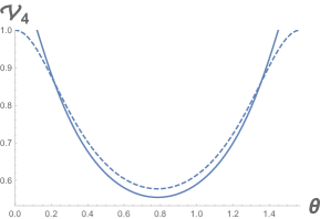
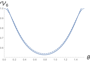
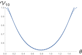
Figure 2: For $n=4,6,10$, the blue solid curve and dashed lines are the threshold value over the parameter $\theta\in[0,\pi/2]$ for the chained steering inequality and the linear steering inequality, respectively.

V Conclusions

We have constructed new $n$-setting chained steering inequalities with the lowest visibility compared with the linear steering inequalities and the chained steering inequalities in Meng . For the generalized Werner states, it has been found that when parameter $\theta$ of the states lies in some neighborhood of $\frac{\pi}{4}$, the new chained steering inequalities always have lower visibility and thus more robust against noise than the $n$-setting steering inequalities. Subsequently, we shall try to construct optimal steering inequalities that have genuine minimal threshold values of quantum violation.

- (1) R. Horodecki, P. Horodecki, M. Horodecki, and K. Horodecki, Rev. Mod. Phys. 81, 865 (2009).
- (2) M. A. Nielsen and I. L. Chuang, Quantum Computation and Quantum Information (Cambridge University Press, Cambridge, England, 2010).
- (3) E. Schrdinger, Proc. Camb. Phil. Soc. 31, 555-563 (1935).
- (4) A. Einstein, B. Podolsky, and N. Rosen, Phys. Rev. 47, 777 (1935).
- (5) H. M. Wiseman, S. J. Jones, and A. C. Doherty, Phys. Rev. Lett. 98, 140402 (2007).
- (6) J. S. Bell, Phys. 1, 195-200 (1964).
- (7) N. Gisin, Phys. Lett. A 154, 201 (1991).
- (8) R. F. Werner, J. Phys. A: Math. Theor. 47, 424008 (2014).
- (9) J. L. Chen, X. J. Ye, C. F. Wu, H. Y. Su, A. Cabello, L. C. Kwek, and C. H. Oh, Sci. Rep. 3, 2143 (2013).
- (10) P. Skrzypczyk, M. Navascues, and D. Cavalcanti, Phys. Rev. Lett. 112, 180404 (2014).
- (11) J. Bowles, T. Vertesi, M. T. Quintino, and N. Brunner, Phys. Rev. Lett. 112, 200402 (2014).
- (12) J. L. Chen, H. Y. Su, Z. P. Xu, and A. K. Pati, Sci. Rep. 6, 32075 (2016).
- (13) J. L. Chen, C. L. Ren, C. B. Chen, X. J. Ye, and A. K. Pati, Sci. Rep. 6, 39063 (2016).
- (14) E. G. Cavalcanti, S. J. Jones, H. M. Wiseman, and M. D. Reid, Phys. Rev. A 80, 032112 (2009).
- (15) D. J. Saunders, S. J. Jones, H. M. Wiseman, and G. J. Pryde, Nature Phys. 6, 845 (2010).
- (16) K. Sun, J. S. Xu, X. J. Ye, Y. C. Wu, J. L. Chen, C. F. Li, and G. C. Guo, Phys. Rev. Lett. 113, 140402 (2014).
- (17) C. Branciard, E. G. Cavalcanti, S. P. Walborn, V. Scarani, and H. M. Wiseman, Phys. Rev. A 85, 010301(R) (2012).
- (18) N. Brunner, D. Cavalcanti, S. Pironio, V. Scarani, and S. Wehner, Rev. Mod. Phys. 86, 419 (2014).
- (19) H. X. Meng, J. Zhou, S. H. Jiang, Z. P. Xu, C. L. Ren, H. Y. Su, and J. L. Chen, to appear in Opt. Commun, DOI: 10.1016/j.optcom.2018.04.074.