IPMU18-0101

Big Bang Nucleosynthesis Constraint on
Baryonic Isocurvature Perturbations

Keisuke Inomata^a,b, Masahiro Kawasaki^a,b, Alexander Kusenko^b,c, Louis Yang^b

^aICRR, The University of Tokyo, Kashiwa, Chiba 277-8582, Japan
^bKavli IPMU (WPI), UTIAS, The University of Tokyo, Kashiwa, Chiba 277-8583, Japan
^cDepartment of Physics and Astronomy, University of California, Los Angeles, CA 90095-1547, USA

1 Introduction

Light elements such as ⁴He and D are synthesized at the cosmic temperature $T$ around $0.1$ MeV. The abundances of light elements predicted by the big-bang nucleosynthesis (BBN) are in good agreement with those inferred from the observations, which has supported the standard hot big-bang cosmology since 1960’s (for review see, [1]). The BBN is very sensitive to physical conditions at $T\simeq 1-0.01$ MeV and hence it is an excellent probe to the early universe. For example, an extra radiation component existing $T\sim 1$ MeV changes the predicted abundances of ⁴He and D and could spoil the success of the BBN, which gives a stringent constraint on the extra radiation energy.

In modern cosmology it is believed that the hot universe is produced after inflation which is an accelerated expansion of the universe and solves several problems in the standard cosmology. One of the most important roles of inflation is a generation of density perturbations. During inflation light scalar fields, including the inflaton, acquire quantum fluctuations which become classical by the accelerated expansion and leads to density perturbations. If only one scalar field ($=$ inflaton) is involved in generation of the density perturbations the produced perturbations are adiabatic and nearly scale invariant, which perfectly agrees with the observations of the CMB and large scale structures on large scales ($\gtrsim\mathcal{O}(10)$ Mpc). The amplitude of the power spectrum of the curvature perturbations is precisely determined as $\mathcal{P}_{\zeta}=2.1\times 10^{-9}$ at the pivot scale $k=0.002~{}\text{Mpc}^{-1}$ by the CMB observations [2].

However, as for small scales we know little about the shape and amplitude of the power spectrum of the density perturbations and there are a few constraints on the curvature perturbations from the CMB $\mu$-distortion due to the Silk dumping [3] and overproduction of primordial black holes [4]. The BBN also gives constraints on the amplitude of the curvature perturbations since they can affect $n/p$ and/or baryon-to-photon ratio through the second order effects and hence change the abundance of the light elements [5, 6, 7] .

Inflation produces not only the curvature (adiabatic) perturbations but also the isocurvature ones. The isocurvature perturbations are produced when multiple scalar fields are involved in generation of the density perturbations. In particular, when scalar fields play an important role in baryogenesis, baryonic isocurvature perturbations are generally produced. A well-known example is the Affleck-Dine baryogenesis [8] where a scalar quark has a large field value during inflation and generates baryon number through dynamics after inflation. This baryogenesis scenario produces the baryonic isocurvature perturbations unless the scalar quark has a large mass in the phase direction [9, 10]. Since the CMB observations are quite consistent with the curvature perturbations, the isocurvature perturbations on the CMB scales are stringently constrained [11]. However, there are almost no constraints on small-scale isocurvature perturbations.

In this paper we show that large baryonic isocurvature perturbations existing at the BBN epoch ($T\sim 0.1$ MeV) change the D abundance by their second order effect. Because the primordial abundance of D is precisely measured with accuracy about 1 % [12, 13], we can obtain a significant constraint on the amplitude $\mathcal{P}_{S_{B}}$ of the baryonic isocurvature perturbations. It is found that the amplitude should be $\mathcal{P}_{S_{B}}\lesssim 0.016\,(2\sigma)$ for scale $k^{-1}\gtrsim 0.0025$ pc. We also apply the constraint to the relaxation leptogenesis scenario [14, 15] where large fluctuations of a scalar field play a crucial role in leptogenesis and large baryonic isocurvature perturbations are predicted. We show that the BBN gives a significant constraint on this scenario.

The paper is organized as follows. In Sec. 2 we briefly review the measurement of the D abundance. We show how the baryonic isocurvature perturbations change the D abundance and obtain a generic constraint on their amplitude in Sec. 3. In Sec. 4 we apply the BBN constraint on the relaxation leptogenesis scenario. Sec. 5 is devoted for conclusions.

2 Deuterium abundance

Light elements like D, ³He and ⁴He are synthesized in the early Universe at temperature $T\simeq 1~{}\text{MeV}-0.01~{}\text{MeV}$. This big bang nucleosynthesis predicts the abundances of light elements which are in agreement with those inferred by observations. In particular, the deuterium abundance has been precisely measured by observing absorption of QSO lights due to damped Lyman-$\alpha$ systems. Most recently Zavaryzin et al. [12] reported the primordial D abundance,

$$(\text{D}/\text{H})_{p}=(2.545\pm 0.025)\times 10^{-5},$$ (1)

from measurements of 13 damped Lyman-$\alpha$ systems. Here $\text{D}/\text{H}$ is the ratio of the number densities of D and H. The observed abundance should be compared with the theoretical prediction. The D abundance produced in BBN is calculated by numerically solving the nuclear reaction network and in the standard case the result is only dependent on the baryon density $\Omega_{B}$. We adopt the following fitting formula in Ref. [2]:

$$10^{5}(\text{D}/\text{H})_{p}=18.754-1534.4\,\omega_{B}+48656\,\omega_{B}^{2}-552670\,\omega_{B}^{3},$$ (2)

where $\omega_{B}=\Omega_{B}h^{2}$ and $h$ is the Hubble constant in units of 100km/s/Mpc. This formula is obtained using the PArthENoPE code [16] and its uncertainty is $\pm 0.12(2\sigma)$. The observational constraint Eq. (1) and the prediction Eq. (2) are shown in Fig. 1. From the figure the BBN prediction is consistent with the observed abundance for $\Omega_{B}h^{2}\simeq 0.022-0.023$.

The baryon density is also precisely determined by CMB observations. The recent Plank measurement gives

$$\Omega_{B}h^{2}=0.02226\pm 0.00023,$$ (3)

which is also shown in Fig. 1. It is seen that the baryon densities determined by BBN and CMB are consistent. However, if the predicted D abundance increases by about 3% in the case with $2\sigma$ uncertainties, they become inconsistent and hence any effect that increases the D abundance is stringently constrained.

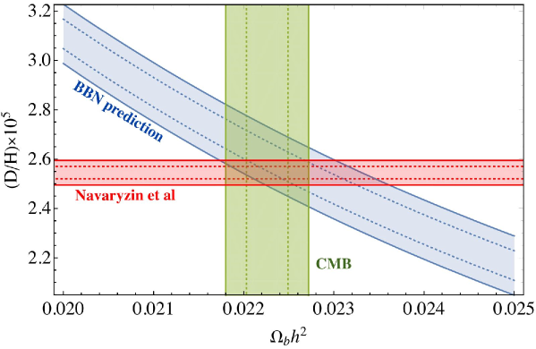
Figure 1: BBN prediction of deuterium as a function of the baryon density is shown by the blue band. The CMB constraint on the baryon density (green) and the observed D abundance (red) are also shown. The dotted (solid) lines denote the contours of $1\sigma$ ($2\sigma$) uncertainties.

3 Baryonic isocurvature perturbations and deuterium abundance

Here we assume that only baryon number fluctuations are produced in the early universe. Such fluctuations are called baryonic isocurvature density perturbations $S_{B}$ which are written as

$$S_{B}=\frac{\delta n_{B}}{n_{B}}-\frac{3}{4}\frac{\delta\rho_{\gamma}}{\rho_{\gamma}}=\frac{\delta n_{B}}{n_{B}},$$ (4)

where $\rho_{\gamma}$ and $\delta\rho_{\gamma}$ are the photon energy density and its perturbation, and we have used the above assumption of the nonexistence of photon perturbations in the last equality.

When the baryon number density has spatial fluctuations it can affect the BBN and change the abundance of light elements. In particular, modification of the D abundance is important because it is precisely determined by the recent measurement. Let us consider the BBN prediction of D in the presence of the baryon number fluctuations by using Eq. (2). In order to take into account the baryon number fluctuations, we consider $\omega_{B}$ in Eq. (2) as space dependent variable,

$$\omega_{B}(t,\vec{x})=\bar{\omega}_{B}+\delta\omega_{B}(\vec{x}),$$ (5)

where $\bar{\omega}_{B}$ is the homogeneous part and $\delta\omega_{B}$ denotes the fluctuations which are related to $S_{B}$ as

$$\delta\omega_{B}=\bar{\omega}_{B}\frac{\delta n_{B}(\vec{x})}{n_{B}}=\bar{\omega}_{B}S_{B}(\vec{x}).$$ (6)

With $\bar{\omega}_{B}$ and $S_{B}$, Eq. (2) is rewritten as

$$y_{d}= 18.754-1534.4\,\bar{\omega}_{B}+48656\,\bar{\omega}_{B}^{2}-552670\,\bar{\omega}_{B}^{3}$$

$$+(-1534.4\,\bar{\omega}_{B}+97312\,\bar{\omega}_{B}^{2}-1658010\,\bar{\omega}_{B}^{3})\,S_{B}$$

$$+(48656\,\bar{\omega}_{B}^{2}-1658010\,\bar{\omega}_{B}^{3})\,S_{B}^{2}+\ldots,$$ (7)

where $y_{d}=10^{5}(\text{D}/\text{H})_{p}$. Since D production takes place at $T\simeq 0.1$ MeV we estimate $S_{B}$ at that time. To estimate the primordial D abundance we should average $y_{d}$ over the volume $V$ corresponding to the present horizon. Using $\langle S_{B}\rangle=0$, we obtain

$$\langle y_{d}\rangle= 18.754-1534.4\,\bar{\omega}_{B}+48656\,\bar{\omega}_{B}^{2}-552670\,\bar{\omega}_{B}^{3}$$

$$+(48656\,\bar{\omega}_{B}^{2}-1658010\,\bar{\omega}_{B}^{3})\,\langle S_{B}^{2}\rangle,$$ (8)

where $\langle\cdots\rangle$ denotes the spatial average. Thus, the D abundance is modified from the homogeneous case owing to the second order effect of the baryonic isocurvature perturbations. The prediction for $\langle S_{B}^{2}\rangle=0.016$ is shown in Fig. 2. It is seen that the isocurvature perturbations increase the D abundance and hence increase the baryon density accounting for the observed abundance, which leads to inconsistency between the baryon densities inferred from CMB and BBN. Thus we can obtain a constraint on $\langle S_{B}^{2}\rangle$.

In order to derive the upper bound on the isocurvature perturbations, we define the discrepancy $\mathcal{D}$ between the observational and theoretical values in the units of standard deviation as

$$\mathcal{D}\equiv\frac{|y_{\text{obs,mean}}-y_{\text{th,mean}}|}{\sqrt{\sigma^{2}_{y_{\text{obs}}}+\sigma^{2}_{y_{\text{th}}}}},$$ (9)

where $y_{\text{obs,mean}}$ and $y_{\text{th,mean}}$ are the mean values of the observation and theoretical prediction and $\sigma^{2}_{\text{obs}}$ and $\sigma^{2}_{\text{th}}$ are the standard deviations of $y_{\text{obs}}$ and $y_{\text{th}}$. Note that $y_{\text{th,mean}}$ and $\sigma_{y_{\text{th}}}$ are calculated by Eq. (8) and therefore they depend on $\langle S_{B}^{2}\rangle$. Imposing the conditions, $\mathcal{D}<1$ or $\mathcal{D}<2$, we can get the constraints on the isocurvature perturbations as $\langle S_{B}^{2}\rangle<0.0020$ ($1\sigma$) or $\langle S_{B}^{2}\rangle<0.016$ ($2\sigma$).

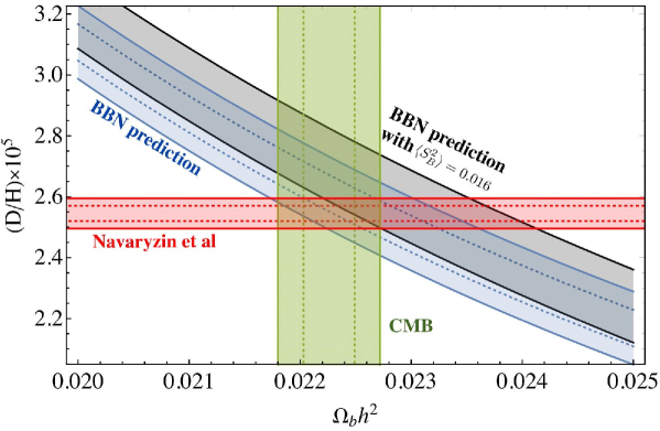
Figure 2: The same as Fig. 1, except that we show the $2\sigma$ BBN prediction in the case with $\langle S_{B}^{2}\rangle=0.016$ by the gray shaded region. Note that the overlap between the region of the D observation and BBN prediction does not necessarily mean the consistence between them.

Let us calculate $\langle S_{B}^{2}\rangle$ from the Fourier mode $S_{B}(\vec{k})$ as

$$\langle S_{B}^{2}\rangle =\frac{1}{V}\int_{V}d^{3}x(S_{B}(\vec{x}))^{2}$$

$$=\frac{1}{(2\pi)^{6}V}\int_{V}d^{3}x\int d^{3}k\int d^{3}k^{\prime}S_{B}(\vec{k})S_{B}^{*}(\vec{k^{\prime}})e^{i(\vec{k}-\vec{k^{\prime}})\cdot\vec{x}}$$

$$=\frac{1}{(2\pi)^{3}}\int d^{3}k|S_{B}(\vec{k})|^{2}=\int d\ln k\,\mathcal{P}_{S_{B}}(k),$$ (10)

where $\mathcal{P}_{S_{B}}(k)$ is the power spectrum of the baryonic isocurvature perturbations. Here we should pay attention to the upper limit of the $k$-integration. The baryons diffuse in the early universe, which erases the baryon number fluctuations with their wavelength less than the diffusion length. So the upper limit of the integration is the wave number $k_{d}$ which corresponds to the diffusion length at the BBN epoch ($T\simeq 0.1$ MeV). The diffusion length of neutrons $d_{n}$ is much larger than that of protons, so $k_{d}$ is given by $d_{n}^{-1}$. The neutron diffusion is determined by neutron-proton scatterings and the comoving diffusion length is given by [17]

$$d_{n}\simeq k_{d}^{-1}\simeq 0.0025\,\text{pc}~{}~{}~{}~{}~{}\text{at }~{}T=0.1\,\text{MeV}.$$ (11)

Thus, $\langle S_{B}^{2}\rangle$ is given by

$$\langle S_{B}^{2}\rangle=\frac{1}{(2\pi)^{3}}\int^{k_{d}}_{k_{*}}d^{3}kP_{S_{B}}(k).$$ (12)

Here $k_{*}$ is the scale corresponding to the present horizon ($k_{*}^{-1}\simeq 3000h^{-1}$ Mpc).

Here, let us summarize the constraints on power spectra of baryonic isocurvature perturbations. In addition to the BBN constraint, which we have discussed so far, there are constraints from the observations of the CMB anisotropy and large scale structure (LSS) [11, 18, 19]. From the CMB anisotropy observations, the effective cold dark matter (CDM) isocurvature perturbations are constrained as (95% CL) [11]

$$\begin{cases}\beta_{\text{iso,CDM}}(k_{\text{low}})<0.045&(k_{\text{low}}=0.002\,\text{Mpc}^{-1})\\ \beta_{\text{iso,CDM}}(k_{\text{mid}})<0.379&(k_{\text{mid}}=0.05\,\text{Mpc}^{-1})\\ \beta_{\text{iso,CDM}}(k_{\text{high}})<0.594&(k_{\text{high}}=0.1\,\text{Mpc}^{-1}).\end{cases}$$ (13)

$\beta_{\text{iso,CDM}}(k)$ is defined as

$$\beta_{\text{iso,CDM}}(k)\equiv\frac{\mathcal{P}_{S_{\text{CDM,eff}}}(k)}{\mathcal{P}_{\zeta}(k)+\mathcal{P}_{S_{\text{CDM,eff}}}(k)},$$ (14)

where $\mathcal{P}_{S_{\text{CDM,eff}}}$ is the power spectrum of the effective CDM isocurvature perturbations, which is defined as $S_{\text{CDM,eff}}=S_{\text{CDM}}+\frac{\Omega_{B}h^{2}}{\Omega_{\text{CDM}}h^{2}}S_{\text{B}}$ with the CDM energy density parameter $\Omega_{\text{CDM}}h^{2}(=0.119)$. In the case with baryonic isocurvature perturbations but without CDM ones, the relation $\mathcal{P}_{S_{\text{CDM,eff}}}=\left(\frac{\Omega_{B}h^{2}}{\Omega_{\text{CDM}}h^{2}}\right)^{2}\mathcal{P}_{S_{B}}$ is satisfied. Then we can convert the constraints on $\mathcal{P}_{S_{\text{CDM,eff}}}$ into those on $\mathcal{P}_{S_{B}}$. Meanwhile, from the combination of the LSS, such as the Lyman-$\alpha$ forest anisotropy, and CMB observations, the isocurvature perturbations are constrained as (95% CL) [18]

$$A_{\text{iso,bar}}=-0.06^{+0.35}_{-0.34},$$ (15)

where $A^{2}_{\text{iso,bar}}\equiv\mathcal{P}_{S_{B}}(k_{0})/\mathcal{P}_{\zeta}(k_{0})$ ($k_{0}=0.05$ Mpc^-1) and this constraint is based on the assumptions that the spectral index of the isocurvature perturbations is the same as that of the curvature perturbations and the isocurvature perturbations are fully correlated with the curvature perturbations. A positive value of $A_{\text{iso,bar}}$ means the full positive correlation and a negative one means the full negative (or anti-) correlation. Note that the Lyman-$\alpha$ forest observations can see the power spectra in smaller scale ($k\lesssim 1$ Mpc^-1) than the CMB observations can ($k\lesssim 0.1$ Mpc^-1).

To visualize the BBN constraints, we assume that the power spectrum is monochromatic as

$$\mathcal{P}_{S_{B},\text{mono}}(k;k_{*})=\mathcal{P}_{S_{B}}\delta(\text{log}k-\text{log}k_{*}).$$ (16)

With this monochromatic power spectrum, the equation $\langle S_{B}^{2}\rangle=\mathcal{P}_{S_{B}}$ is satisfied. In Fig. 3, we show the $\mathcal{P}_{S_{B}}$ region excluded by the BBN observations with orange shaded one. For comparison, we show also the constraints from the CMB and LSS observations given by Eqs. (13) and (15). Regarding the combination constraint in Fig. 3, to show the conservative constraint, we assume the full negative correlation and take $A_{\text{iso,bar}}=-0.40$. Note that the derived constraint on $\langle S_{B}^{2}\rangle$ is valid even in the compensated isocurvature perturbations [20], in which the CDM isocurvature perturbation totally compensates the baryonic one, because BBN occurs during radiation era and is independent of CDM perturbations.

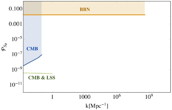
Figure 3: The summary of the constraints on baryonic isocurvature perturbations. An orange shaded region is excluded by the D observations, which we derived in this paper. A blue shaded region is excluded by the CMB observations [11]. For comparison, we plot also the constraints from the combination of CMB and LSS observations with a green dotted line [18], though this constraint is based on some assumptions (see text).

Before closing this section, we discuss the applicability of Eq. (2) to the inhomogeneous BBN. Since D is synthesized in a rather short period ($T=0.1$–$0.05$ MeV), we can focus on only that period. The most important scale in our problem is the diffusion length. In Eq. (12) we take the neutron diffusion length $d_{n}$ as a cutoff because the proton diffusion length $d_{p}$ is about $100$ times shorter than $d_{n}$ [17]. If the fluctuation wavelength $k^{-1}$ of baryons are larger than the neutron diffusion scale $d_{n}$, the diffusion does not play an important role and D production takes place in locally homogeneous regions, which justifies the use of Eq. (2). Thus, our generic constraint in Fig. 3 is valid for $k<k_{d}=d_{n}^{-1}$. On the other hand, if $k^{-1}$ is smaller than the proton diffusion length, diffusion makes baryons homogeneous, so again we can use Eq. (2). The complicated situation occurs when the fluctuation scale is $d_{n}^{-1}<k<d_{p}^{-1}$. To see how BBN is affected by such fluctuations, let us consider a region with size $d_{n}$. In this region neutrons are homogeneous but protons fluctuate, which produces high and low proton sub-regions in a homogeneous neutron region. In high proton sub-regions BBN proceeds a little earlier than in low proton sub-regions, which leads to more ⁴He and hence less D. Because the fluctuations are perturbative, the net result is the same as the homogeneous BBN in the first order. However, if we take the second order effect into account, we have to consider the diffuse-back of neutrons. In the high proton sub-regions neutron are consumed for D production earlier and neutron density becomes smaller than the low proton sub-regions. Then neutrons in the low proton sub-region diffuse into the high proton sub-regions and those neutrons are consumed. Thus, as a net result, D could decrease by the second order effect. Since it is difficult to estimate this effect quantitatively, we assume that the effect is small in this paper.

4 Relaxation leptogenesis

One model capable of generating the baryonic isocurvature perturbations is the relaxation leptogenesis [14, 27, 15]. In this section, we will briefly review the relaxation leptogenesis framework and discuss the improved constraint from the deuterium abundance on this type of models. In the relaxation leptogenesis framework, the generation of lepton/baryon asymmetry is driven by the classical motion of a scalar field $\phi$ during the period of cosmic inflation and the following reheating stage of the universe. During inflation, a light scalar field $\phi$ with mass $m_{\phi}<H_{I}$ can develop a large nonzero vacuum expectation value (VEV) $\phi_{0}\equiv\sqrt{\left\langle\phi^{2}\right\rangle}$ through quantum fluctuations [28, 29, 30]. If the quantum fluctuation is not suppressed by the potential or other interactions, the $\phi$ can reach an equilibrium VEV $\phi_{0}$ satisfying $V\left(\phi_{0}\right)\sim H_{I}^{4}$, where $H_{I}=\Lambda_{I}^{2}/\sqrt{3}M_{pl}$ is the Hubble rate during inflation, and $\Lambda_{I}$ is the inflationary energy scale.

However, in general, one can expect there are interactions between $\phi$ and the inflaton field $I$ of the form

$$\mathcal{L}_{\phi I}=\lambda_{\phi I}\frac{\left(\phi^{\dagger}\phi\right)^{m/2}\left(I^{\dagger}I\right)^{n/2}}{M_{pl}^{m+n-4}}.$$ (17)

In the early stage of the inflation when the inflaton VEV $\left\langle I\right\rangle$ is large, interactions like Eq. (17) can contribute a large effective mass term [$m_{\phi}\left(I\right)\gg H_{I}$] to $\phi$ suppressing the quantum fluctuations of $\phi$. As the inflaton VEV $\left\langle I\right\rangle$ decreases in the later stage of inflation, $\phi$ becomes lighter. When the effective mass of $\phi$ falls below $m_{\phi}\left(I\right)<H_{I}$, the quantum fluctuations of $\phi$ can start to grow. If the VEV of $\phi$ only develops in the last $N_{\mathrm{last}}$ $e$-folds of inflation, its VEV can reach $\phi_{0}\simeq\sqrt{N_{\mathrm{last}}}H_{I}/2\pi$. This is the “IC-2” scenario considered in [14, 15].

During reheating, the VEV of $\phi$ relaxes to the minimum of the potential and oscillates with decreasing amplitudes. The relaxation of $\phi$ provides the out of thermal equilibrium condition and breaks time-reversal symmetry, allowing baryogenesis to proceed. For successful relaxation leptogenesis, one considers the derivative coupling between the $\phi$ and the $B+L$ fermion current $j_{B+L}^{\mu}$ of the form

$$\mathcal{O}_{6}=-\frac{1}{\Lambda_{n}^{2}}\left(\partial_{\mu}\left|\phi\right|^{2}\right)j_{B+L}^{\mu},$$ (18)

for some higher energy scale $\Lambda_{n}$. This operator can be treated as an effective chemical potential for the fermion current $j_{B+L}$ as $\phi$ evolves in time. In the presence of a $B$ or $L$-violating process, the system can then relax toward a state with nonzero $B$ or $L$.

In the case of Higgs relaxation leptogenesis ($\phi=h$), the final lepton asymmetry, $Y\equiv n_{L}/s$, is estimated to be [31]

$$Y\approx\dfrac{90\sigma_{R}}{\pi^{6}g_{*S}}\left(\dfrac{\phi_{0}}{\Lambda_{n}}\right)^{2}\dfrac{3z_{0}T_{RH}}{4\alpha_{T}t_{RH}}\exp\left(-\dfrac{8+\sqrt{15}}{\pi^{2}}\sigma_{R}T_{RH}^{3}t_{RH}\right),$$ (19)

if the Higgs potential is dominated by the thermal mass term $V\left(\phi,T\right)\approx\frac{1}{2}\alpha_{T}^{2}T^{2}\phi^{2}$ during reheating. The parameters for Eq. (19) are $\alpha_{T}\approx 0.33$ at the energy scale $\mu\sim 10^{13}$ GeV, $g_{*S}=106.75$, and $z_{0}=3.376$. $\sigma_{R}$ is the thermally averaged cross section of the $L$-violating process, which we consider to be the scattering between left-handed neutrinos via the exchange of a heavy right-handed neutrino. $\phi_{0}$ is the initial VEV of the Higgs field at the end of inflation, which depends on $N_{\mathrm{last}}$. The reheating channel is assumed to be perturbative with the reheat temperature $T_{RH}\simeq\left(24/\pi^{2}g_{*}\right)^{1/4}\sqrt{M_{pl}/t_{RH}}$ when reheating is complete at $t_{RH}$. The produced lepton asymmetry then turns into baryon asymmetry through the Sphaleron process and becomes the baryon density of the universe as the universe cools down.

Since the asymmetry generated in this manner depends crucially on the initial VEV $\phi_{0}$, the spatial fluctuation of $\phi$ due to quantum fluctuation at inflation stage can result in baryonic perturbations at later time. These perturbations are isocurvature modes because the scalar field $\phi$ is not the inflaton $I$ and doesn’t dominate the energy density of the universe. As we have discussed in previous sections, baryonic isocurvature perturbations are constrained by observations in both the amplitude and the spatial scale $k$. Thus, we can translate these into the constraints on the $N_{\mathrm{last}}$ of the Higgs field and other inflation parameters like $\Lambda_{I}$ and $T_{RH}$.

As computed in Ref. [31], the power spectrum of the baryon density perturbations resulted from the quantum fluctuation of $\phi$ is

$$\mathcal{P}_{S_{B}}\left(k\right)\approx\frac{4}{N_{\mathrm{last}}^{2}}\ln\left(\frac{k}{k_{s}}\right)\theta\left(k-k_{s}\right)\theta\left(k_{s}e^{N_{\mathrm{last}}}-k\right),$$ (20)

for the fluctuation of $\phi$ only developed in the last $N_{\mathrm{last}}$ $e$-fold of inflation. Here $k_{s}\sim a\left(N_{\mathrm{last}}\right)H_{I}$ is the comoving wave number corresponding to the mode which first leaves the horizon. By considering a typical inflation setup with the inflationary energy scale $\Lambda_{I}$ and the reheat temperature $T_{RH}$, we can then relate $k_{s}$ and $N_{\mathrm{last}}$ by

$$k_{s}\simeq 2\pi e^{-N_{\mathrm{last}}}H_{I}\left(\frac{T_{RH}}{\Lambda_{I}}\right)^{4/3}\frac{g_{*S}^{1/3}\left(T_{\mathrm{now}}\right)}{g_{*S}^{1/3}\left(T_{RH}\right)}\frac{T_{\mathrm{now}}}{T_{RH}},$$ (21)

or

$$k_{s}e^{N_{\mathrm{last}}}\simeq 65\,\mathrm{Mpc}^{-1}e^{46.3}\equiv k_{s,\,0}\,e^{N_{0}},$$ (22)

for $\Lambda_{I}=10^{16}\,\mathrm{GeV}$, $T_{RH}=10^{12}\,\mathrm{GeV}$, and $T_{\mathrm{now}}=2.726\,\mathrm{K}$.

The square of the baryonic isocurvature perturbations $\left\langle S_{B}^{2}\right\rangle$ is then given by

$$\left\langle S_{B}^{2}\right\rangle =\int_{k_{*}}^{k_{d}}\frac{dk}{k}\mathcal{P}_{S_{B}}\left(k\right)$$ (23)

$$\approx\frac{4}{N_{\mathrm{last}}^{2}}\int_{k_{*}}^{k_{d}}\frac{dk}{k}\ln\left(\frac{k}{k_{s}}\right)\theta\left(k-k_{s}\right)\theta\left(k_{s}e^{N_{\mathrm{last}}}-k\right)$$ (24)

$$=\frac{2}{N_{\mathrm{last}}^{2}}\min\left[\ln^{2}\left(\frac{k_{d}}{k_{s}}\right)\theta\left(k_{d}-k_{s}\right),\,N_{\mathrm{last}}^{2}\right],$$ (25)

where in the last step we have assumed $k_{*}<k_{s}$. With Eq. (22), we have

$$\left\langle S_{B}^{2}\right\rangle=\frac{2}{N_{\mathrm{last}}^{2}}\left[\ln\left(\frac{k_{d}}{k_{s,\,0}}\right)+N_{\mathrm{last}}-N_{0}\right]^{2}\theta\left(k_{d}-k_{s}\right).$$ (26)

The constraint on baryonic isocurvature perturbation from the D abundance then gives an upper bound on $N_{\mathrm{last}}$ as

$$N_{\mathrm{last}}\lesssim 33.7\quad\text{(}2\sigma\text{)},$$ (27)

for $\Lambda_{I}=10^{16}\,\mathrm{GeV}$ and $T_{RH}=10^{12}\,\mathrm{GeV}$.

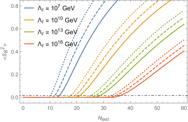
Figure 4: The baryonic isocurvature perturbations $\left\langle S_{B}^{2}\right\rangle$ generated by the Higgs relaxation leptogenesis at various $N_{\mathrm{last}}$ and $\Lambda_{I}$. The solid, dashed, and dotted lines correspond to the cases where the reheat temperatures $T_{RH}$ are $10^{-1}\Lambda_{I}$, $10^{-3}\Lambda_{I}$, and $10^{-5}\Lambda_{I}$, respectively. The gray horizontal dash-dot line at $\langle S_{B}^{2}\rangle=0.016$ indicates the constraint from the D abundance at $2\sigma$ level.

Figure 4 shows the baryonic isocurvature perturbations generated by the Higgs relaxation leptogenesis model at various $N_{\mathrm{last}}$ and $\Lambda_{I}$. We see that larger values of $\Lambda_{I}$ and $T_{RH}$ allowing for larger $N_{\mathrm{last}}$. We also see that for each choice of parameters ($\Lambda_{I}$, $T_{RH}$), there is a minimum $N_{\mathrm{last}}$ below which the fluctuation $\left\langle S_{B}^{2}\right\rangle$ becomes zero. This corresponds to the case when the scale of the produced baryonic perturbations is smaller than the baryon diffusion scale $k_{d}$. So the baryonic perturbation is washed out by neutron diffusion before the BBN.

Figure 5 shows the parameter space in $\Lambda_{I}$ vs $N_{\mathrm{last}}$ at various reheat temperatures $T_{RH}$. Note that the CMB observations from Planck gives an upper bound on the inflationary energy scale $\Lambda_{I}<1.88\times 10^{16}\,\text{GeV}$ [11]. For successful Thus, for a given set of $\Lambda_{I}$ and $T_{RH}$, the D abundance constraint provides an upper bound on $N_{\mathrm{last}}$.

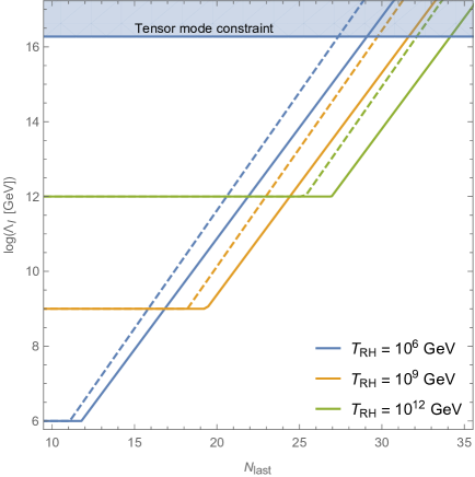
Figure 5: The BBN constraint on the Higgs relaxation leptogenesis in the $\Lambda_{I}$-$N_{\mathrm{last}}$ space at various reheat temperature $T_{RH}$. The dashed (solid) lines correspond to the 1$\sigma$ (2$\sigma$) constraints. The regions on the lower right side of each contours are excluded. The blue shaded region for $\Lambda_{I}>1.88\times 10^{16}\,\text{GeV}$ is constrained by Planck non-observation of tensor mode [11]. For successful inflation, one also requires $\Lambda_{I}>T_{RH}$, which is indicated as the horizontal parts of each contours.

5 Conclusion

We have shown that large baryonic isocurvature perturbations existing at the BBN epoch ($T\sim 0.1$ MeV) change the D abundance by the second order effect, which, together with the recent precise D measurement with accuracy about $1$ %, leads to a constraint on the amplitude of the power spectrum $\mathcal{P}_{S_{B}}$ of the baryon isocurvature perturbations. It is found that the amplitude should be $\mathcal{P}_{S_{B}}\lesssim 0.016\,(2\sigma)$ for scale $k^{-1}\gtrsim 0.0025$ pc [see Fig. 3]. Since there has been no constraint on baryonic isocurvature perturbations on small scale $k^{-1}<10$ Mpc, the BBN constraint obteined in this paper is the most stringent one for $0.1\,\text{Mpc}^{-1}\lesssim k\lesssim 4\times 10^{8}\,\text{Mpc}^{-1}$. Moreover, this constraint is valid even if the perturbations are compensated isocurvature perturbations because BBN can be affected only by the baryonic perturbations.

We have also applied the BBN constraint to the relaxation leptogenesis scenario where large baryon isocurvature perturbations are produced in the last $N_{\text{last}}$ $e$-fold of inflation. It is found that the upper bound on $N_{\text{last}}$ is imposed as $N_{\text{last}}\lesssim 34$ for $T_{R}\lesssim 10^{12}$ GeV from the BBN constraint on baryonic isocurvature perturbations.

References

- [1] F. Iocco, G. Mangano, G. Miele, O. Pisanti and P. D. Serpico, Primordial Nucleosynthesis: from precision cosmology to fundamental physics, Phys. Rept. 472 (2009) 1–76, [0809.0631].
- [2] Planck collaboration, P. A. R. Ade et al., Planck 2015 results. XIII. Cosmological parameters, Astron. Astrophys. 594 (2016) A13, [1502.01589].
- [3] J. Chluba and D. Grin, CMB spectral distortions from small-scale isocurvature fluctuations, Mon. Not. Roy. Astron. Soc. 434 (2013) 1619–1635, [1304.4596].
- [4] B. J. Carr, K. Kohri, Y. Sendouda and J. Yokoyama, New cosmological constraints on primordial black holes, Phys. Rev. D81 (2010) 104019, [0912.5297].
- [5] D. Jeong, J. Pradler, J. Chluba and M. Kamionkowski, Silk damping at a redshift of a billion: a new limit on small-scale adiabatic perturbations, Phys. Rev. Lett. 113 (2014) 061301, [1403.3697].
- [6] T. Nakama, T. Suyama and J. Yokoyama, Reheating the Universe Once More: The Dissipation of Acoustic Waves as a Novel Probe of Primordial Inhomogeneities on Even Smaller Scales, Phys. Rev. Lett. 113 (2014) 061302, [1403.5407].
- [7] K. Inomata, M. Kawasaki and Y. Tada, Revisiting constraints on small scale perturbations from big-bang nucleosynthesis, Phys. Rev. D94 (2016) 043527, [1605.04646].
- [8] I. Affleck and M. Dine, A New Mechanism for Baryogenesis, Nucl. Phys. B249 (1985) 361–380.
- [9] K. Enqvist and J. McDonald, Observable isocurvature fluctuations from the Affleck-Dine condensate, Phys. Rev. Lett. 83 (1999) 2510–2513, [hep-ph/9811412].
- [10] S. Kasuya, M. Kawasaki and F. Takahashi, Isocurvature fluctuations in Affleck-Dine mechanism and constraints on inflation models, JCAP 0810 (2008) 017, [0805.4245].
- [11] Planck collaboration, P. A. R. Ade et al., Planck 2015 results. XX. Constraints on inflation, Astron. Astrophys. 594 (2016) A20, [1502.02114].
- [12] E. O. Zavarygin, J. K. Webb, S. Riemer-Sørensen and V. Dumont, Primordial deuterium abundance at z=2.504 towards Q1009+2956, 2018, 1801.04704, http://inspirehep.net/record/1648127/files/arXiv:1801.04704.pdf.
- [13] R. J. Cooke, M. Pettini and C. C. Steidel, One Percent Determination of the Primordial Deuterium Abundance, Astrophys. J. 855 (2018) 102, [1710.11129].
- [14] A. Kusenko, L. Pearce and L. Yang, Postinflationary Higgs relaxation and the origin of matter-antimatter asymmetry, Phys. Rev. Lett. 114 (2015) 061302, [1410.0722].
- [15] L. Yang, L. Pearce and A. Kusenko, Leptogenesis via Higgs Condensate Relaxation, Phys. Rev. D92 (2015) 043506, [1505.07912].
- [16] O. Pisanti, A. Cirillo, S. Esposito, F. Iocco, G. Mangano, G. Miele et al., PArthENoPE: Public Algorithm Evaluating the Nucleosynthesis of Primordial Elements, Comput. Phys. Commun. 178 (2008) 956–971, [0705.0290].
- [17] J. H. Applegate, C. J. Hogan and R. J. Scherrer, Cosmological Baryon Diffusion and Nucleosynthesis, Phys. Rev. D35 (1987) 1151–1160.
- [18] U. Seljak, A. Slosar and P. McDonald, Cosmological parameters from combining the Lyman-alpha forest with CMB, galaxy clustering and SN constraints, JCAP 0610 (2006) 014, [astro-ph/0604335].
- [19] M. Beltran, J. Garcia-Bellido, J. Lesgourgues and M. Viel, Squeezing the window on isocurvature modes with the lyman-alpha forest, Phys. Rev. D72 (2005) 103515, [astro-ph/0509209].
- [20] C. Gordon and A. Lewis, Observational constraints on the curvaton model of inflation, Phys. Rev. D67 (2003) 123513, [astro-ph/0212248].
- [21] D. Grin, D. Hanson, G. P. Holder, O. Doré and M. Kamionkowski, Baryons do trace dark matter 380,000 years after the big bang: Search for compensated isocurvature perturbations with WMAP 9-year data, Phys. Rev. D89 (2014) 023006, [1306.4319].
- [22] J. B. Muñoz, D. Grin, L. Dai, M. Kamionkowski and E. D. Kovetz, Search for Compensated Isocurvature Perturbations with Planck Power Spectra, Phys. Rev. D93 (2016) 043008, [1511.04441].
- [23] J. Valiviita, Power Spectra Based Planck Constraints on Compensated Isocurvature, and Forecasts for LiteBIRD and CORE Space Missions, JCAP 1704 (2017) 014, [1701.07039].
- [24] T. Haga, K. Inomata, A. Ota and A. Ravenni, Exploring compensated isocurvature perturbations with CMB spectral distortion anisotropies, 1805.08773.
- [25] M. T. Soumagnac, R. Barkana, C. G. Sabiu, A. Loeb, A. J. Ross, F. B. Abdalla et al., Large-Scale Distribution of Total Mass versus Luminous Matter from Baryon Acoustic Oscillations: First Search in the Sloan Digital Sky Survey III Baryon Oscillation Spectroscopic Survey Data Release 10, Phys. Rev. Lett. 116 (2016) 201302, [1602.01839].
- [26] M. T. Soumagnac, C. G. Sabiu, R. Barkana and J. Yoo, Large scale distribution of mass versus light from Baryon Acoustic Oscillations: Measurement in the final SDSS-III BOSS Data Release 12, 1802.10368.
- [27] L. Pearce, L. Yang, A. Kusenko and M. Peloso, Leptogenesis via neutrino production during Higgs condensate relaxation, Phys. Rev. D92 (2015) 023509, [1505.02461].
- [28] A. D. Linde, Scalar Field Fluctuations in Expanding Universe and the New Inflationary Universe Scenario, Phys. Lett. B116 (1982) 335–339.
- [29] A. A. Starobinsky, Dynamics of Phase Transition in the New Inflationary Universe Scenario and Generation of Perturbations, Phys. Lett. B117 (1982) 175–178.
- [30] A. Vilenkin and L. H. Ford, Gravitational Effects upon Cosmological Phase Transitions, Phys. Rev. D26 (1982) 1231.
- [31] M. Kawasaki, A. Kusenko, L. Pearce and L. Yang, Relaxation leptogenesis, isocurvature perturbations, and the cosmic infrared background, Phys. Rev. D95 (2017) 103006, [1701.02175].