Accelerating Incremental Gradient Optimization with Curvature Information

Abstract

This paper studies an acceleration technique for incremental aggregated gradient (IAG) method through the use of curvature information for solving strongly convex finite sum optimization problems. These optimization problems of interest arise in large-scale learning applications. Our technique utilizes a curvature-aided gradient tracking step to produce accurate gradient estimates incrementally using Hessian information. We propose and analyze two methods utilizing the new technique, the curvature-aided IAG (CIAG) method and the accelerated CIAG (A-CIAG) method, which are analogous to gradient method and Nesterov’s accelerated gradient method, respectively. Setting $\kappa$ to be the condition number of the objective function, we prove the $R$ linear convergence rates of $1-\frac{4c_{0}\kappa}{(\kappa+1)^{2}}$ for the CIAG method, and $1-\sqrt{\frac{c_{1}}{2\kappa}}$ for the A-CIAG method, where $c_{0},c_{1}\leq 1$ are constants inversely proportional to the distance between the initial point and the optimal solution. When the initial iterate is close to the optimal solution, the $R$ linear convergence rates match with the gradient and accelerated gradient method, albeit CIAG and A-CIAG operate in an incremental setting with strictly lower computation complexity. Numerical experiments confirm our findings. The source codes used for this paper can be found on http://github.com/hoitowai/ciag/.

1 Introduction

Consider a finite sum optimization problem with $m$ component functions and a $d$-dimensional decision variable:

$$\textstyle\min_{\bm{\theta}\in\mathbb{R}^{d}}~{}F(\bm{\theta})\mathrel{\mathop{:}}=\sum_{i=1}^{m}f_{i}(\bm{\theta})\;.$$ (1)

Problem (1) is motivated by the empirical risk minimization model where we are learning a parameter $\bm{\theta}$ from a finite set of data. The component function $f_{i}(\bm{\theta})$ represents the statistical mismatch between $\bm{\theta}$ and the $i$th piece of data collected. The aim of problem (1) is to learn the optimal parameter, denoted by $\bm{\theta}^{\star}$, that fits with the $m$ available data points vapnik1999overview .

We are interested in the setting when each of the component function $f_{i}(\bm{\theta})$ is twice continuously differentiable and the sum function $F(\bm{\theta})$ is strongly convex. Especially, this paper focuses on large-scale instances of (1) with $m\gg 1$. The difficulty with solving (1) lies in the overwhelming size of $m$, which prohibits us from even applying simple first order methods. For example, the full gradient (FG) requires the recursion: let $\gamma>0$ be a step size,

$$\textstyle\bm{\theta}^{k+1}=\bm{\theta}^{k}-\gamma\sum_{i=1}^{m}{\nabla}f_{i}(\bm{\theta}^{k})\;,$$ (2)

that involves a computation cost of ${\cal O}(md)$ floating point operations (FLOPS) per iteration to compute the sum of $m$ gradient vectors. As $m\gg 1$, this is undesirable from a practical standpoint. To this end, a popular yet powerful approach is to adopt the so-called incremental (or stochastic) methods where only one of the component functions, e.g., the $i_{k}$th one, $f_{i_{k}}(\bm{\theta})$, is explored at the $k$th iteration. Examples include the incremental gradient (IG) bertsekas2011incremental , incremental aggregated gradient (IAG) blatt2007convergent ; vanli2016stronger ; gurbuzbalaban2017convergence methods when $i_{k}$ is deterministic; and the stochastic gradient (SG) robbins1951stochastic , stochastic average gradient (SAG) schmidt2017minimizing , SAGA defazio2014saga , stochastic variance reduced gradient (SVRG) xiao2014proximal methods when $i_{k}$ is chosen randomly. Related work can be found in mairal2015incremental ; so2017non for the case with non-convex functions; in lan2017optimal for the cases of finite-sum and primal-dual optimization; in nedic2001convergence ; nedic2001incremental for the case with non-smooth functions. The interested readers are referred to (bottou2016optimization, , Section 4, 5) for a comprehensive overview on the topic.

A number of the above incremental methods achieve linear convergence via the variance reduction technique, e.g., xiao2014proximal ; defazio2014saga ; schmidt2017minimizing . In the worst case, these methods require $k={\cal O}(m\log(1/\epsilon))$ iterations to guarantee that they compute an $\epsilon$-optimal solution $\bm{\theta}^{k}$ satisfying $F(\bm{\theta}^{k})-F(\bm{\theta}^{\star})\leq\epsilon$. In problem instances when $m\gg 1$, such rates may not be ideal. In fact, recent work agarwal2015lower ; arjevani2016dimension ; lan2017optimal showed that the dependence on $m$ is necessary for incremental methods whose updates are linear combinations of the first order information. To improve the convergence rate of incremental methods, a recent direction is to adopt ideas of second-order optimization. Examples include gurbuzbalaban2015globally ; rodomanov2016superlinearly ; mokhtari2017iqn which extended Newton and quasi-Newton methods to the incremental setting, resulting in NIM rodomanov2016superlinearly and IQN mokhtari2017iqn . These works demonstrated that at the expense of additional storage or computation cost, it is possible to achieve local but superlinear convergence.

We propose a curvature-aided gradient tracking technique for accelerating incremental gradient methods using the curvature (Hessian) information. By applying Taylor expansion on the component functions’ gradients, we derive a new gradient estimator whose error depends on the squares of the optimality gaps. Based on this new gradient tracking technique, we propose two incremental gradient methods, called Curvature-aided Incremental Aggregated Gradient (CIAG) method and Accelerated CIAG (A-CIAG) method. The proposed methods require ${\cal O}(md)$ storage cost and ${\cal O}(d^{2})$ computation cost per iteration. Furthermore, we characterize the $R$-linear convergence rates of the proposed methods. For the CIAG (resp. A-CIAG) method, we show that the rate is $1-\frac{4c_{0}\kappa}{(\kappa+1)^{2}}$ (resp. $1-\sqrt{\frac{c_{1}}{2\kappa}}$), where $\kappa$ is the conditional number of the objective function of the summed objective function $F(\bm{\theta})$ in (1), $c_{0},c_{1}$ are constants which can be set to $1$ given that the initial iterate is close to the optimal solution [cf. Theorems 1 and 2]. In addition, we establish the $R$-linear convergence rates for two non-linear inequalities [cf. Propositions 5 and 6] which are of independent interest. In detail, our result reveals that the convergence of CIAG and A-CIAG methods depends on the initialization, and the trajectory of convergence can be divided into two phases — the initial phase that exhibits a slow but global linear rate; and the asymptotic phase that exhibits linear convergence of an accelerated rate.

A comparison of the proposed CIAG/A-CIAG methods to state-of-the-art methods is summarized in Table 1. Compared to first order methods such as SAG, we remark that the proposed methods (as well as SVRG2, IQN, NIM) require the Hessian of the objective function to be Lipschitz continuous. Though the storage requirement for the proposed methods is ${\cal O}(md+d^{2})$ which is higher than the ${\cal O}(md)$ requirement of the SAG methods when $d\gg 1$, the number of iterations required is significantly lower when the desired accuracy is high, $\epsilon\ll 1$. Overall, as seen from Table 1, the proposed methods are desired when $d$ is small-to-moderate, and the number of component functions $m$ is large.

	Storage	Comp.	# iterations to $\epsilon$-optimal solution
IAG blatt2007convergent	${\cal O}(md)$	${\cal O}(d)$	${\cal O}(m\!~{}\kappa\log(1/\epsilon))$ [worst-case]
SAG schmidt2017minimizing	${\cal O}(md)$	${\cal O}(d)$	${\cal O}(\max\{\kappa,m\}\log(1/\epsilon))$ [expected]
SAGA defazio2014saga	${\cal O}(md)$	${\cal O}(d)$	${\cal O}((\kappa+m)\log(1/\epsilon))$ [expected]
SVRG xiao2014proximal	${\cal O}(d)$	${\cal O}(d)$	${\cal O}((\kappa+m)\log(1/\epsilon))$ [expected]
AccSVRG nitanda2014stochastic	${\cal O}(d)$	${\cal O}(d)$	${\cal O}((m\sqrt{\kappa}+m)\log(1/\epsilon))$ [expected]
SVRG2 gower2017tracking	${\cal O}(d^{2})$	${\cal O}(d^{2})$	${\cal O}(\kappa\log(1/\epsilon)+m)$ [expected]
IQN mokhtari2017iqn	${\cal O}(md^{2})$	${\cal O}(d^{2})$	${\cal O}(m)$, i.e., super-linear [worst-case]
NIM rodomanov2016superlinearly	${\cal O}(md+d^{2})$	${\cal O}(d^{3})$	${\cal O}(m)$, i.e., super-linear [worst-case]
CIAG (proposed)	${\cal O}(md+d^{2})$	${\cal O}(d^{2})$	${\cal O}({\kappa}\log(1/\epsilon)+m)$ [worst-case]
A-CIAG (proposed)	${\cal O}(md+d^{2})$	${\cal O}(d^{2})$	${{\cal O}(\sqrt{\kappa}\log(1/\epsilon)+m)}$ [worst-case]

Table 1: Comparison of state-of-the-art methods for the strongly convex problem (1). The second column is the memory required for the working variables. The third column is the per iteration computation complexity in FLOPS. The last column is the (expected or worst-case) number of iterations to reach an $\epsilon$-optimal solution. SVRG, AccSVRG, SVRG2 require recomputing the full gradient at every epoch and a careful tuning of the epoch size. The constant $\kappa$ is the condition number of $F(\bm{\theta})$ [see (3) and (4) for the definition]. The rates for the last four methods are asymptotic, i.e., they hold only when the desired accuracy is small, e.g., $\epsilon\ll 1$. The shaded rows denote the proposed methods which achieve a good trade-off between per-iteration complexity and convergence speed.

It is worth mentioning that recently in gower2017tracking the authors proposed a method that incorporates Hessian information to accelerate SVRG method, giving the SVRG2 method. The authors developed approximation techniques to reduce the per iteration complexity from ${\cal O}(d^{2})$ to ${\cal O}(d)$. The best convergence rates achieved therein match that of the FG method and is the same as the CIAG method. However, we note that SVRG2 re-computes the full Hessian at the beginning of each epoch. This costs an additional ${\cal O}(md^{2})$ FLOPS per epoch and the cost is negligible only when the epochs are long, e.g., when the epoch lengths are ${\cal O}(m)$.

Organization. Section 2 studies incremental algorithms with gradient tracking and introduces the curvature-aided gradient tracking technique. Section 3 describes the proposed CIAG and A-CIAG methods, and discusses the implementation issues. Section 4 provides the main convergence results. Section 5 demonstrates the efficacy of the proposed methods via numerical experiments.

Notations. We use ${\bm{0}}$ to denote an all-zero vector/matrix with suitable dimensions. Unless otherwise specified, we denote by $\|\cdot\|$ the Euclidean norm. A function $f:\mathbb{R}^{d}\rightarrow\mathbb{R}$ is $L$-smooth if

$$f(\bm{\theta}^{\prime})\leq f(\bm{\theta})+\langle{\nabla}f(\bm{\theta}),\bm{\theta}^{\prime}-\bm{\theta}\rangle+(L/2)\|\bm{\theta}^{\prime}-\bm{\theta}\|^{2}\;,$$ (3)

for $\bm{\theta},\bm{\theta}^{\prime}\in\mathbb{R}^{d}$, and it is $\mu$-strongly convex if

$$f(\bm{\theta}^{\prime})\geq f(\bm{\theta})+\langle{\nabla}f(\bm{\theta}),\bm{\theta}^{\prime}-\bm{\theta}\rangle+(\mu/2)\|\bm{\theta}^{\prime}-\bm{\theta}\|^{2}\;,$$ (4)

for $\bm{\theta},\bm{\theta}^{\prime}\in\mathbb{R}^{d}$. Define $\kappa(f)\mathrel{\mathop{:}}=L/\mu$ as the condition number of $f$. Also, $f$ has an $L_{H}$-Lipschitz continuous Hessian if

$$\|{\nabla}^{2}f(\bm{\theta}^{\prime})-{\nabla}^{2}f(\bm{\theta})\|\leq L_{H}\|\bm{\theta}^{\prime}-\bm{\theta}\|,~{}\forall~{}\bm{\theta},\bm{\theta}^{\prime}\in\mathbb{R}^{d}\;,$$ (5)

where the norm on the left hand side is the matrix norm induced by Euclidean norm. For a non-negative scalar sequence $\{a^{(k)}\}_{k\geq 1}$, we say that it converges $R$-linearly at a rate $\rho$ if the sequence satisfies $\lim_{k\rightarrow\infty}a^{(k+1)}/a^{(k)}=\rho$, where $0\leq\rho<1$. We use standard Bachmann-Landau notations for asymptotic quantities: $a^{(k)}={\cal O}(f^{(k)})$ (resp. $a^{(k)}=\Omega(g^{(k)})$) implies that there exists $k_{0}\in\mathbb{Z}_{+}$ and non-negative constant $C_{1}$ (resp. $C_{2}$) such that $a^{(k)}\leq C_{1}f^{(k)}$ (resp. $a^{(k)}\geq C_{2}g^{(k)}$) for all $k\geq k_{0}$.

2 Gradient Tracking in Incremental Methods

We provide a high-level description of how to incorporate curvature information to accelerate incremental aggregated gradient method. To set up the notation, let $i_{k}\in\{1,...,m\}$ be the component function index selected at the $k$th iteration, e.g., a simple rule is to use the cyclic rule as $i_{k}=(k~{}{\rm mod}~{}m)+1$, or we may choose $i_{k}\sim{\cal U}\{1,...,m\}$. Let us define:

$$\tau_{i}^{k}\mathrel{\mathop{:}}=\max\{\tau:\tau\leq k,~{}i_{\tau}=i\}\;,$$ (6)

i.e., $\tau_{i}^{k}$ is the iteration index where the $i$th component function is last accessed after the completion of the $k$th iteration. As we focus on analyzing the worst-case performance, we assume that $\tau_{i}^{k}\in[k-K+1,k]$ for a constant $K={\cal O}(m)$. For example, $K=m$ when $i_{k}$ is chosen by the cyclic rule.

First-order Approximation. As described in (2), at the $k$th iteration the gradient method computes the full gradient as the complete sum $\sum_{i=1}^{m}{\nabla}f_{i}(\bm{\theta}^{k})$. Such vector is unavailable in the incremental setting as only the access to the $i_{k}$th function is desired. A simple idea is to replace the full gradient by:

$$\textstyle{\bm{g}}_{\sf IAG}^{k}\mathrel{\mathop{:}}=\sum_{i=1}^{m}{\nabla}f_{i}(\bm{\theta}^{\tau_{i}^{k}})\approx\sum_{i=1}^{m}{\nabla}f_{i}(\bm{\theta}^{k})\;,$$ (7)

or equivalently using the recursion:

$${\bm{g}}_{\sf IAG}^{k}={\bm{g}}_{\sf IAG}^{k-1}-{\nabla}f_{i_{k}}(\bm{\theta}^{\tau_{i_{k}}^{k-1}})+{\nabla}f_{i_{k}}(\bm{\theta}^{k})\;,$$ (8)

with ${\bm{g}}_{\sf IAG}^{0}=\sum_{i=1}^{m}{\nabla}f_{i}(\bm{\theta}^{0})$. The expression (7) describes the SAG and IAG methods, where their only differences lie in the selection strategy for $i_{k}$.

When the functions $f_{i}$ are smooth, we have $\|{\nabla}f_{i}(\bm{\theta}^{\tau_{i}^{k}})-{\nabla}f_{i}(\bm{\theta}^{k})\|={\cal O}(\|\bm{\theta}^{\tau_{i}^{k}}-\bm{\theta}^{k}\|)$. Furthermore, gurbuzbalaban2017convergence shows that the error is bounded:

$${\textstyle\|{\bm{g}}_{\sf IAG}^{k}-\sum_{i=1}^{m}{\nabla}f_{i}(\bm{\theta}^{k})\|}={\cal O}\big{(}\gamma m\max_{i=1,...,m}\|\bm{\theta}^{\star}-\bm{\theta}^{\tau_{i}^{k}}\|\big{)}.$$ (9)

Note that this error represents the ‘variance’ in gradient estimation. Eq. (9) implies that the tracking error decays to zero as long as $\bm{\theta}^{k}$ converges to $\bm{\theta}^{\star}$ [recall that $k-\tau_{i}^{k}\leq K<\infty$ and $K=\Theta(m)$]. However, the dependency on $m$ of the right hand side in (9) is undesirable as it leads to the following estimates:

$$\begin{split}\|\bm{\theta}^{k+1}-\bm{\theta}^{\star}\|^{2}&\leq\big{(}1-{\cal O}(\text{\scriptsize$\frac{\gamma}{\kappa(F)}$})\big{)}\|\bm{\theta}^{k}-\bm{\theta}^{\star}\|^{2}+{\cal O}(\gamma^{2}m^{2}\max_{(k-2K)_{++}\leq\ell\leq k}\|\bm{\theta}^{\ell}-\bm{\theta}^{\star}\|^{2})\;,\end{split}$$ (10)

where $(x)_{++}\mathrel{\mathop{:}}=\max\{1,x\}$. As analyzed by gurbuzbalaban2017convergence ; feyzmahdavian2014delayed , due to the dependence of $m^{2}$ on the right hand side, the sequence of squared norm $\{\|\bm{\theta}^{k}-\bm{\theta}^{\star}\|^{2}\}_{k\geq 1}$ converges only when $\gamma={\cal O}(1/m)$, and finally this shows that $\|\bm{\theta}^{k}-\bm{\theta}^{\star}\|^{2}$ converges linearly at rate $1-{\cal O}(1/(m^{2}\kappa(F)))$. Notice that a recent work vanli2016stronger strengthened this rate to $1-{\cal O}(1/(m\kappa(F)))$. When the component function $i_{k}$ is selected independently at random for each $k$, the rate may also be improved, see schmidt2017minimizing .

Second-order Approximation. The undesirable $m$-dependence of convergence rate with (7) is partly due to the crude approximation ${\nabla}f_{i}(\bm{\theta}^{k})\approx{\nabla}f_{i}(\bm{\theta}^{\tau_{i}^{k}})$ used. As a natural idea to improve the approximation, we consider the Taylor expansion applied on the $i$th gradient vector itself:

$${\nabla}f_{i}(\bm{\theta}^{k})\approx{\nabla}f_{i}(\bm{\theta}^{\tau_{i}^{k}})+{\nabla}^{2}f_{i}(\bm{\theta}^{\tau_{i}^{k}})(\bm{\theta}^{k}-\bm{\theta}^{\tau_{i}^{k}})\;.$$ (11)

Compared to a first order approximation with ${\nabla}f_{i}(\bm{\theta}^{k})\approx{\nabla}f_{i}(\bm{\theta}^{\tau_{i}^{k}})$, the approximation given by the right hand side in (11) has two important features. First, we observe that this term yields a second-order approximation to the gradient of the component function $f_{i}(\bm{\theta})$ evaluated at $\bm{\theta}^{k}$, and thus leading to an improved approximation. Second, the approximate term on the right hand side does not require access to the $i$th function evaluated at $\bm{\theta}^{k}$, which allows one to derive a similar recursion rule as (8) to incrementally compute the approximation.

To further evaluate the approximation quality given by (11), for each $i$ we shall assume that the Hessian of $f_{i}$ is Lipschitz continuous. We observe the following upper bound on the error:

Lemma 1

(nesterov2013introductory, , Lemma 1.2.5) Assume that ${\nabla}^{2}f_{i}(\bm{\theta})$ is $L_{H,i}$ Lipschitz. Then:

$$\begin{split}&\big{\|}{\nabla}f_{i}(\bm{\theta})-\big{(}{\nabla}f_{i}(\bm{\theta}^{\prime})+{\nabla}^{2}f_{i}(\bm{\theta}^{\prime})(\bm{\theta}-\bm{\theta}^{\prime})\big{)}\big{\|}\leq(L_{H,i}/2)\|\bm{\theta}-\bm{\theta}^{\prime}\|^{2},~{}\forall~{}\bm{\theta},\bm{\theta}^{\prime}\in\mathbb{R}^{d}\;.\end{split}$$ (12)

From Lemma 1, we notice that the approximation error of the right hand side in (11) depends on the squared difference between $\bm{\theta}^{k}$ and $\bm{\theta}^{\tau_{i}^{k}}$. When $\bm{\theta}^{k}$ is close to $\bm{\theta}^{\tau_{i}^{k}}$, this error will be significantly smaller than what is obtained for the first order approximation methods in (7). We remark that similar approximation schemes are proposed in recent work zheng2017asynchronous ; gower2017tracking , which demonstrated the benefits of applying higher-order approximation in stochastic optimization.

We refer to this form of gradient approximation in (11) as the curvature-aided gradient tracking technique. In the remainder of this paper, we shall develop and analyze practical optimization methods using the technique.

Algorithm 1 CIAG and A-CIAG Method.

1:  Input: Initial point $\bm{\theta}^{1}\in\mathbb{R}^{d}$, step size parameter $\gamma>0$, (for A-CIAG only) extrapolation constant $\alpha$.

2:  Initialize the vectors/matrices in the memory:

$$\bm{\theta}_{i}^{1}=\bm{\theta}^{1},~{}\tau_{i}^{1}=0,~{}\forall~{}i,~{}{\bm{b}}^{0}={\bm{0}},~{}{\bm{H}}^{0}={\bm{0}}\;.\vspace{-.5cm}$$ (13)

3:  for $k=1,2,\dots$ do

4:      Select $i_{k}\in\{1,...,m\}$, e.g., $i_{k}=(k~{}{\rm mod}~{}m)+1$, and the algorithm is given access to $f_{i_{k}}(\bm{\theta})$. Set the counter variables as $\tau_{i_{k}}^{k}=k$, $\tau_{j}^{k}=\tau_{j}^{k-1}$ for all $j\neq i_{k}$.

5:     (For A-CIAG only) If $k=1$, we take $\bm{\theta}_{ex}^{1}=\bm{\theta}^{1}$; otherwise we compute the extrapolated variable as $\bm{\theta}_{ex}^{k}=\bm{\theta}^{k}+\alpha(\bm{\theta}^{k}-\bm{\theta}^{k-1})$.

6:     Update the vector in the memory:

$$\bm{\theta}_{i_{k}}^{k}=\begin{cases}\bm{\theta}^{k},&\text{for {\sf CIAG} \;,}\\ \bm{\theta}_{ex}^{k},&\text{for {\sf A-CIAG} \;,}\end{cases}$$ (14)

and set $\bm{\theta}_{j}^{k}=\bm{\theta}_{j}^{k-1}$ for all $j\neq i_{k}$.

7:      If $\tau_{i_{k}}^{k-1}=0$, then update: (self-initialization)

$$\begin{split}{\bm{b}}^{k}&={\bm{b}}^{k-1}+{\nabla}f_{i_{k}}(\bm{\theta}_{i_{k}}^{k})-{\nabla}^{2}f_{i_{k}}(\bm{\theta}_{i_{k}}^{k})\bm{\theta}_{i_{k}}^{k}\;,\\ {\bm{H}}^{k}&={\bm{H}}^{k-1}+{\nabla}^{2}f_{i_{k}}(\bm{\theta}_{i_{k}}^{k})\;.\\[-8.5359pt] \end{split}$$ (15)

Otherwise, update:

$$\begin{split}{\bm{b}}^{k}&={\bm{b}}^{k-1}-{\nabla}f_{i_{k}}(\bm{\theta}_{i_{k}}^{k-1})+{\nabla}f_{i_{k}}(\bm{\theta}_{i_{k}}^{k})+{\nabla}^{2}f_{i_{k}}(\bm{\theta}_{i_{k}}^{k-1})\bm{\theta}_{i_{k}}^{k-1}-{\nabla}^{2}f_{i_{k}}(\bm{\theta}_{i_{k}}^{k})\bm{\theta}_{i_{k}}^{k}\;,\\ {\bm{H}}^{k}&={\bm{H}}^{k-1}-{\nabla}^{2}f_{i_{k}}(\bm{\theta}_{i_{k}}^{k-1})+{\nabla}^{2}f_{i_{k}}(\bm{\theta}_{i_{k}}^{k})\;.\\[-8.5359pt] \end{split}$$ (16)

8:      Compute the update:

$$\textstyle\bm{\theta}^{k+1}=\bm{\theta}_{i_{k}}^{k}-\gamma\big{(}{\bm{b}}^{k}+{\bm{H}}^{k}\bm{\theta}_{i_{k}}^{k}\big{)}\;.\vspace{-.1cm}$$ (17)

9:  end for

10:  Return: an approximate solution to (1), $\bm{\theta}^{k+1}$.

3 Proposed CIAG and A-CIAG Methods

We propose two incremental methods, CIAG and A-CIAG methods, which are built using the curvature-aided gradient tracking technique (11). Our first method, the CIAG method, performs the recursion:

$$\bm{\theta}^{k+1}=\bm{\theta}^{k}-\gamma{\bm{g}}_{\sf CIAG}^{k}\;,$$ (18)

where $\gamma>0$ is a step size and the gradient surrogate is given by

$$\begin{split}{\bm{g}}_{\sf CIAG}^{k}&\mathrel{\mathop{:}}=\sum_{i=1}^{m}\big{(}{\nabla}f_{i}(\bm{\theta}^{\tau_{i}^{k}})-{\nabla}^{2}f_{i}(\bm{\theta}^{\tau_{i}^{k}})\bm{\theta}^{\tau_{i}^{k}}\big{)}+\Big{(}\sum_{i=1}^{m}{\nabla}^{2}f_{i}(\bm{\theta}^{\tau_{i}^{k}})\Big{)}\bm{\theta}^{k}\;,\end{split}$$ (19)

where $\tau_{i}^{k}$ was defined in (6). The method can be interpreted as applying the curvature-aided gradient tracking [cf. (11)] to each individual component function and applying the FG update (2). On the other hand, the accelerated CIAG (A-CIAG) method follows the recursion:

$$\bm{\theta}_{ex}^{k} =\bm{\theta}^{k}+\alpha(\bm{\theta}^{k}-\bm{\theta}^{k-1})\;,$$ (20a)

$$\bm{\theta}^{k+1} =\bm{\theta}_{ex}^{k}-\gamma{\bm{g}}_{\sf ACIAG}^{k}\;,$$ (20b)

where $\alpha\in[0,1),\gamma>0$ are predefined parameters and the gradient surrogate is

$$\begin{split}{\bm{g}}_{\sf ACIAG}^{k}&\textstyle\mathrel{\mathop{:}}=\sum_{i=1}^{m}\big{(}{\nabla}f_{i}(\bm{\theta}_{ex}^{\tau_{i}^{k}})-{\nabla}^{2}f_{i}(\bm{\theta}_{ex}^{\tau_{i}^{k}})\bm{\theta}_{ex}^{\tau_{i}^{k}}\big{)}+\Big{(}\sum_{i=1}^{m}{\nabla}^{2}f_{i}(\bm{\theta}_{ex}^{\tau_{i}^{k}})\Big{)}\bm{\theta}_{ex}^{k}\;,\\[0.0pt] \end{split}$$ (21)

where $\tau_{i}^{k}$ was defined in (6). The term $\bm{\theta}_{ex}^{k}$ in (20a) is called the extrapolated iterate, which incorporates the ‘inertia’ from previous iterates into the updates. Similar to the CIAG method, the A-CIAG method applies curvature-aided gradient tracking to the gradient of each individual component function, evaluated at $\bm{\theta}_{ex}^{k}$. We remark that even though Hessians are used in the CIAG and A-CIAG methods, we do not attempt to compute any matrix inverses which is in contrast with Newton methods. The Hessians here are used to accelerate the gradient tracking.

The CIAG and A-CIAG methods are similar since the full gradients evaluated at $\bm{\theta}^{k}$ and $\bm{\theta}_{ex}^{k}$ are approximated by their respective curvature-aided gradient tracking approximates [cf. (19) & (21)]. Both methods can be implemented in a memory efficient incremental fashion. To see this, define

$$\bm{\theta}_{i}^{k}\mathrel{\mathop{:}}=\begin{cases}\bm{\theta}^{\tau_{i}^{k}},&\text{for {\sf CIAG} \;,}\\ \bm{\theta}_{ex}^{\tau_{i}^{k}},&\text{for {\sf A-CIAG} \;,}\end{cases}~{}~{}{\bm{H}}^{k}\mathrel{\mathop{:}}=\sum_{i=1}^{m}{\nabla}^{2}f_{i}(\bm{\theta}_{i}^{k}),$$ (22)

and

$$\textstyle{\bm{b}}^{k}\mathrel{\mathop{:}}=\sum_{i=1}^{m}\big{(}{\nabla}f_{i}(\bm{\theta}_{i}^{k})-{\nabla}^{2}f_{i}(\bm{\theta}_{i}^{k})\bm{\theta}_{i}^{k}\big{)}\;.$$ (23)

Note that ${\bm{b}}^{k}$ and ${\bm{H}}^{k}$ are the accumulated staled iterates, gradients and Hessians. These can be computed incrementally through storing the staled iterates in memory. Moreover, we can compute the gradient surrogates as ${\bm{g}}_{\sf CIAG}^{k}={\bm{b}}^{k}+{\bm{H}}^{k}\bm{\theta}^{k}$ and ${\bm{g}}_{\sf ACIAG}^{k}={\bm{b}}^{k}+{\bm{H}}^{k}\bm{\theta}_{ex}^{k}$. A pseudo code for implementing CIAG and A-CIAG is provided in Algorithm 1.

3.1 Computation and Storage Costs

We comment on the computation and storage costs of CIAG and A-CIAG. Note that (15), (16) and (17) in the algorithm require ${\cal O}(d^{2})$ FLOPS and they are the dominant computation steps involved. The overall complexities for CIAG and A-CIAG are thus ${\cal O}(d^{2})$ FLOPS per iteration. On the other hand, the algorithm requires storing $m$ vectors of $d$-dimesion and a $d\times d$ matrix [cf. (13)], therefore the storage cost is ${\cal O}(md+d^{2})={\cal O}(md)$ if $m\geq d$. When $d$ is small, the computation and storage cost of CIAG and A-CIAG are comparable to existing methods such as SAG, SVRG; meanwhile for large $d$, the computation cost will be undesirable for CIAG and A-CIAG.

When the component functions are the negative log-likelihood of a linear model, the storage complexity can be reduced to as low as ${\cal O}(m)$. Note linear models are common in machine learning problems. We write

$$f_{i}(\bm{\theta})=g_{i}(\langle\bm{\theta},{\bm{x}}_{i}\rangle)+(\rho/2)\|\bm{\theta}\|^{2}\;,\vspace{-.1cm}$$ (24)

where ${\bm{x}}_{i}$ represents the $i$th associated data, while $g_{i}:\mathbb{R}\rightarrow\mathbb{R}$ is twice continuously differentiable. Observe that

$$\begin{split}&{\nabla}f_{i}(\bm{\theta})=g_{i}^{\prime}(\langle\bm{\theta},{\bm{x}}_{i}\rangle){\bm{x}}_{i}+\rho\!~{}\bm{\theta},~{}{\nabla}^{2}f_{i}(\bm{\theta})=g_{i}^{\prime\prime}(\langle\bm{\theta},{\bm{x}}_{i}\rangle){\bm{x}}_{i}({\bm{x}}_{i})^{\top}+\rho{\bm{I}}\;,\end{split}\vspace{-.1cm}$$ (25)

where ${\bm{I}}$ is the $d\times d$ identity matrix. Substituting the above into (16) gives:

$$\begin{split}{\bm{b}}^{k}&={\bm{b}}^{k-1}+(g_{i_{k}}^{\prime}(\langle\bm{\theta}_{i_{k}}^{k},{\bm{x}}_{i_{k}}\rangle)-g_{i_{k}}^{\prime}(\langle\bm{\theta}_{i_{k}}^{k-1},{\bm{x}}_{i_{k}}\rangle)){\bm{x}}_{i_{k}}\\ &+g_{i_{k}}^{\prime\prime}(\langle\bm{\theta}_{i_{k}}^{k-1},{\bm{x}}_{i_{k}}\rangle)\langle\bm{\theta}_{i_{k}}^{k-1},{\bm{x}}_{i_{k}}\rangle{\bm{x}}_{i_{k}}-g_{i_{k}}^{\prime\prime}(\langle\bm{\theta}_{i_{k}}^{k},{\bm{x}}_{i_{k}}\rangle)\langle\bm{\theta}_{i_{k}}^{k},{\bm{x}}_{i_{k}}\rangle{\bm{x}}_{i_{k}}\vspace{.1cm}\\ \end{split}$$ (26)

$${\bm{H}}^{k}={\bm{H}}^{k-1}+(g_{i_{k}}^{\prime\prime}(\langle\bm{\theta}_{i_{k}}^{k},{\bm{x}}_{i_{k}}\rangle)-g_{i_{k}}^{\prime\prime}(\langle\bm{\theta}_{i_{k}}^{k-1},{\bm{x}}_{i_{k}}\rangle)){\bm{x}}_{i_{k}}{\bm{x}}_{i_{k}}^{\top}\;.$$ (27)

Therefore, it suffices for CIAG and A-CIAG to keep $\{\langle{\bm{x}}_{i},\bm{\theta}_{i}\rangle\}_{i=1}^{m}$ for implementing the incremental updates, leading to an ${\cal O}(d^{2}+m)$ storage cost.

4 Convergence Analysis

In this section, we demonstrate that the proposed methods converge globally and characterize their convergence rates. Let us state the assumptions.

Assumption 1

The delayed iteration indices $\tau_{i}^{k}$ [cf. (6)] satisfy $0\leq k-\tau_{i}^{k}\leq K$ for all $i,k$ and for some $K\geq 0$.

Assumption 2

The function $F(\bm{\theta})$ is $\mu$-strongly convex and $L$-smooth with $L\geq\mu>0$.

Assumption 3

For each $i$, the Hessian of the function $f_{i}(\bm{\theta})$ is $L_{H,i}$-Lipschitz continuous.

We define $L_{H}\mathrel{\mathop{:}}=\sum_{i=1}^{m}L_{H,i}$ as the Lipschitz constant for the Hessian of the sum function $F(\bm{\theta})$. The first assumption above can be satisfied when Line 4 of Algorithm 1 is implemented with either cyclic function selection, i.e., $i_{k}=(k~{}{\rm mod}~{}m)+1$, or implemented with a random shuffling step at the beginning of every epoch gurbuzbalaban2015random . The second and the last assumptions are standard and they can be satisfied by a number of functions relevant to machine learning applications, e.g., the logistic loss function.

Let us first present the convergence result for the CIAG method — taking the parameterization $\gamma=c/(\mu+L)$ for some $0<c\leq 2$. We have:

Theorem 1

Let Assumptions 1, 2 and 3 hold. Consider the CIAG method with its optimality gap sequence defined as $V^{(k)}\mathrel{\mathop{:}}=\|\bm{\theta}^{k}-\bm{\theta}^{\star}\|^{2}$ where $\bm{\theta}^{\star}$ is the optimal solution to (1). If the step size parameter, $c$, satisfies:

$$\begin{split}c<\min\Big{\{}&2,~{}\frac{1}{K}\sqrt{\frac{\mu L(\mu+L)}{2L_{H}(L^{2}(V^{(1)})^{\frac{1}{2}}+4L_{H}^{2}(V^{(1)})^{\frac{3}{2}})}},\Big{(}\frac{1}{K^{4}}\frac{\mu L(\mu+L)^{4}}{2L_{H}^{2}(L^{4}V^{(1)}+16L_{H}^{4}(V^{(1)})^{3})}\Big{)}^{1/5}\Big{\}}\;,\end{split}$$ (28)

then there exists $\delta\in[1-2\gamma\frac{\mu L}{L+\mu},1)$ such that the sequence $\{V^{(k)}\}_{k\geq 1}$ converges linearly,

$$V^{(k)}\leq\delta^{\lceil(k-1)/(2K+1)\rceil}V^{(1)},~{}\forall~{}k\geq 1\;.$$ (29)

Moreover, there exists an upper bound sequence $\{\bar{V}^{(k)}\}_{k\geq 1}$, which satisfies $\bar{V}^{(k)}\geq V^{(k)}$ for all $k\geq 1$ and $\bar{V}^{(1)}=V^{(1)}$ such that

$$\begin{split}&\lim_{k\rightarrow\infty}\frac{\bar{V}^{(k+1)}}{\bar{V}^{(k)}}\leq 1-2\gamma\frac{\mu L}{L+\mu}=1-{\cal O}\Big{(}\frac{c}{\kappa(F)}\Big{)}\;.\end{split}$$ (30)

Next, for the A-CIAG method, we adopt the parameters:

$$\alpha=\frac{1-\sqrt{\mu\gamma}}{1+\sqrt{\mu\gamma}},~{}~{}\gamma=\frac{c}{L}\;,$$ (31)

such that the extarpolation factor and step size are controlled by some $0<c\leq 1/2$. Our result is summarized as follows:

Theorem 2

Let Assumptions 1, 2 and 3 hold. Consider the A-CIAG method with its optimality gap sequence defined as $h^{(k)}\mathrel{\mathop{:}}=F(\bm{\theta}^{k})-F(\bm{\theta}^{\star})$. If the step size parameter, $c$, satisfies:

$$c<\min\left\{\bar{c}_{1},\bar{c}_{2},\bar{c}_{3},1/2\right\}\;,$$ (32)

where

$$\bar{c}_{1}\mathrel{\mathop{:}}=\left(\frac{\sqrt{\mu}}{\sqrt{18}K^{2}L_{H}}\frac{L^{2}}{\frac{20L^{2}}{\mu}(2h^{(1)})^{\frac{1}{2}}+\big{(}\frac{40L_{H}}{\mu}\big{)}^{2}(2h^{(1)})^{\frac{3}{2}}}\right)^{\frac{1}{2}},$$ (33)

$$\bar{c}_{2}\mathrel{\mathop{:}}=\left(\frac{2\mu}{81K^{4}L_{H}^{2}}\frac{L^{4}}{\big{(}\frac{20L^{2}}{\mu}\big{)}^{2}(2\bar{h}^{(1)})+\big{(}\frac{40L_{H}}{\mu}\big{)}^{4}(2h^{(1)})^{3}}\right)^{\frac{1}{4}},~{}\bar{c}_{3}\mathrel{\mathop{:}}=\frac{L}{\sqrt{324}K^{2}L_{H}\frac{(h^{(1)})^{\frac{1}{2}}}{\sqrt{\mu}}+1296K^{4}L_{H}^{2}\frac{h^{(1)}}{\mu^{2}}+\mu},$$

then the optimality gap $h^{(k)}$ satisfies

$$h^{(k)}\leq{\delta^{\lceil\frac{k}{2K+1}\rceil}}(2h^{(1)}),~{}\forall~{}k\geq 1\;,$$ (34)

for some $\delta<1$; moreover, there exists an upper bound sequence $\{\bar{h}^{(k)}\}_{k\geq 1}$ such that $\bar{h}^{(k)}\geq h^{(k)}$ for all $k\geq 1$ and $\bar{h}^{(1)}=h^{(1)}$, such that

$$\lim_{k\rightarrow\infty}\frac{\bar{h}^{(k+1)}}{\bar{h}^{(k)}}=1-\sqrt{\mu\gamma}=1-\sqrt{\frac{c}{\kappa(F)}}\;.$$ (35)

The above theorems reveal that there are two phases of convergence for the CIAG and A-CIAG methods – one that converges at a slow linear rate [cf. (29) and (34)], and the asymptotic phase where the algorithms converge linearly at a fast rate comparable to the FG and AFG methods [cf. (30) and (35)]. Such behavior is similar to the linear and superlinear convergence phases in the Newton’s method bertsekas1999nonlinear , and they can be anticipated as the CIAG and A-CIAG methods make use of the second order information.

Due to the strong convexity of $F(\bm{\theta})$ [cf. Assumption 2], the potential function used in the two theorems above are comparable, since

$$\frac{\mu}{2}V^{(k)}\leq h^{(k)}\leq\frac{L}{2}V^{(k)}\Longrightarrow h^{(k)}=\Theta(V^{(k)})\;.$$ (36)

Both theorems require the step size parameters be chosen according to the initial conditions [cf. (28) and (32)]. The allowable range of step size $\gamma$ is inversely proportional to $L_{H}$ and $V^{(1)}$. The former term $L_{H}$ measures the ‘quadratic-ness’ of the component functions such that $L_{H}=0$ if $f_{i}(\bm{\theta})$ are quadratic. The latter term $V^{(1)}$ is the initial optimality gap for the algorithms, which is originated from the use of curvature information. The favorable cases are when $L_{H}\approx 0$ or $V^{(1)}\approx 0$ such that we can take $c\approx 1$. The latter implies the following asymptotic convergence rates:

$$\begin{split}&{\sf CIAG}:\lim_{k\rightarrow\infty}\frac{\bar{V}^{(k+1)}}{\bar{V}^{(k)}}=1-{\cal O}\Big{(}\frac{1}{\kappa(F)}\Big{)},\\ &\text{\sf A-CIAG}:\lim_{k\rightarrow\infty}\frac{\bar{h}^{(k+1)}}{\bar{h}^{(k)}}=1-\sqrt{\frac{1/2}{\kappa(F)}}\;.\end{split}$$ (37)

They coincide with the convergence rates achieved by the FG and AFG methods, respectively. Since the per-iteration complexity of CIAG, A-CIAG are ${\cal O}(d^{2})$, while the complexity of FG, AFG are ${\cal O}(md)$, the advantage of the proposed methods is significant when $m\gg d$. It is also interesting to compare the convergence criterion for the CIAG and A-CIAG methods. Most noticeably, the A-CIAG criterion (33) differs from the CIAG criterion (28) for the region specified by $\tilde{c}_{3}$ as the A-CIAG requires the step size parameter be chosen as $c={\cal O}(1/K^{4})$ for large $K$. Since $K=\Theta(m)$, the initial optimality gap has to be as small as $h^{(1)}={\cal O}(1/m^{4})$ to attain the fast rate as (37). In comparison, the CIAG method only requires $V^{(1)}={\cal O}(1/m^{2})$ to attain (37) due to the milder requirements in (28).

When $V^{(1)}\not\approx 0$ and $L_{H}\not\approx 0$, we can choose a small step size parameter $c$ at the beginning of CIAG (or A-CIAG) method that satisfies (28) (or (33)). By (29) (or (34)), for some finite $T_{0}$, the method is guaranteed to find a solution with $V^{(T_{0}+1)}<V^{(1)}$ after $T_{0}$ iterations. As such, we can ‘re-start’ the method using $\bm{\theta}^{(T_{0}+1)}$ as the initial point with a larger step size parameter $c$. The procedure can then be repeated until $c$ is increased to $c=2$ (or $c=\frac{1}{2}$ for A-CIAG). In this way, the ideal asymptotic convergence rates in (37) are achieved. Alternatively, we can employ other incremental optimization methods such as SAG schmidt2017minimizing to ‘warm-start’ the CIAG or A-CIAG methods with an initial point satisfying $V^{(1)}\approx 0$. We remark that analyzing the exact complexity of a ‘re-starting’ schedule is non-trivial which is beyond the scope of the current paper.

Nevertheless, from our numerical experiments in Section 5, we find that the practical step sizes can often be chosen more aggressively. For a wide range of problems, using a constant step size parameter $c$, the CIAG and A-CIAG methods converge quickly in terms of the number of iterations used and CPU time, without the aforementioned re-starting or warm-starting techniques.

4.1 Proofs of Theorem 1 and 2

The analysis for CIAG and A-CIAG methods consists of three steps.

• First, we carry out a perturbation analysis on the FG and AFG methods. Effectively, we view the CIAG (resp. A-CIAG) method as a perturbed FG (resp. AFG) method with inexact gradients, where the errors are defined as:

  $$\begin{split}&\textstyle{\bm{e}}_{\sf CIAG}^{k}\mathrel{\mathop{:}}={\bm{g}}_{\sf CIAG}^{k}-\sum_{i=1}^{m}{\nabla}f_{i}(\bm{\theta}^{k}),~{}\textstyle{\bm{e}}_{\sf ACIAG}^{k}\mathrel{\mathop{:}}={\bm{g}}_{\sf ACIAG}^{k}-\sum_{i=1}^{m}{\nabla}f_{i}(\bm{\theta}_{ex}^{k})\;.\end{split}$$ (38)

• Second, we analyze an upper bound on $\|{\bm{e}}_{\sf CIAG}^{k}\|$ or $\|{\bm{e}}_{\sf ACIAG}^{k}\|$ in terms of

  $$V^{(k)}\mathrel{\mathop{:}}=\|\bm{\theta}^{k}-\bm{\theta}^{\star}\|^{2},~{}~{}h^{(k)}\mathrel{\mathop{:}}=F(\bm{\theta}^{k})-F(\bm{\theta}^{\star})\;,$$ (39)

  where we shall use $V^{(k)}$, $h^{(k)}$ as the potential functions for CIAG method and A-CIAG method, respectively. Here, we exploited Assumption 3 on the Lipschitz continuity of Hessian for the component functions.

• Third, using the bounds derived in the previous steps we study a nonlinear inequality system to derive the convergence criterion of $V^{(k)}$ and $h^{(k)}$. The nonlinear inequality exhibits the desired $R$-linear convergence when $k\rightarrow\infty$.

Overall, the key to our proof is to analyze the dynamics of optimality gap $V^{(k)}$ (or $h^{(k)}$) as a nonlinear system, whose convergence can be guaranteed by an appropriately chosen step size $\gamma$ and the asymptotic convergence rate will only depend on the linear terms in the optimality gaps.

In the following, we assume that the CIAG, ACIAG methods are both initialized such that (23) holds. This can be done ‘on-the-fly’ with a self-initialization step in (15) and the analysis below will hold for all $k\geq K$, i.e., after a complete pass through the dataset.

Step 1. The first step is to analyze the CIAG (resp. A-CIAG) method as a perturbed version of the FG (resp. AFG) method, which employs ${\bm{g}}_{\sf CIAG}^{k}$ (resp. ${\bm{g}}_{\sf ACIAG}^{k}$) as the gradient surrogate. We have:

Proposition 1

Consider the CIAG method. Under Assumption 2, if $\gamma\leq 2/(\mu+L)$, we have that for all $k\geq 1$,

$$\begin{split}V^{(k+1)}&\leq\Big{(}1-2\gamma\frac{\mu L}{\mu+L}\Big{)}V^{(k)}+\gamma^{2}\|{\bm{e}}_{\sf CIAG}^{k}\|^{2}+2\gamma\sqrt{V^{(k)}}\|{\bm{e}}_{\sf CIAG}^{k}\|\;.\end{split}$$ (40)

The proof largely follows from (gurbuzbalaban2017convergence, , Section 3.3) and is omitted.

Proposition 2

Consider the A-CIAG method. Under Assumption 2, if $\gamma\leq 1/(2L)$, we have that for all $k\geq 1$,

$$\begin{split}h^{(k+1)}&\leq 2(1-\sqrt{\mu\gamma})^{k}h^{(1)}+\sum_{\ell=1}^{k}(1-\sqrt{\mu\gamma})^{k-\ell}\Big{(}\sqrt{2\gamma h^{(\ell)}}\|{\bm{e}}_{\sf ACIAG}^{\ell}\|+\sqrt{\frac{9\gamma}{\mu}}\|{\bm{e}}_{\sf ACIAG}^{\ell}\|^{2}-\frac{\mu}{4}\frac{1-\mu\gamma}{\sqrt{\mu\gamma}}\|\bm{\theta}^{\ell}-\bm{\theta}_{ex}^{\ell}\|^{2}\Big{)}.\end{split}$$ (41)

From the propositions, we observe that when the gradient errors vanish with ${\bm{e}}^{\ell}={\bm{0}}$, setting $\gamma=2/(\mu+L)$ (resp. $\gamma=1/(2L)$) gives $V^{(k+1)}={\cal O}((1-1/\kappa(F))^{k})$ (resp. $h^{(k+1)}={\cal O}((1-\sqrt{1/2\kappa(F)})^{k})$). In other words, the linear convergence rates for FG and AFG methods can be recovered.

Comparing the two propositions reveals the differences in error structure between the CIAG and A-CIAG methods. First, in (41) the A-CIAG’s error is convolved with the linearly converging sequence $(1-\sqrt{\mu\gamma})^{\ell}$, while in (40) the CIAG’s error is simply additive; second, (41) consists of a negative term depending on $\|\bm{\theta}^{\ell}-\bm{\theta}_{ex}^{\ell}\|^{2}$. This negative term revealed through our refined analysis of the error dynamics of A-CIAG [see (81)] and the resultant proposition is an improvement over schmidt2011convergence . Significantly, this negative term is an important key for establishing the fast convergence of A-CIAG.

Step 2. Our next step relates the gradient errors ${\bm{e}}_{\sf CIAG}^{\ell}$, ${\bm{e}}_{\sf ACIAG}^{\ell}$ to the optimality gaps $V^{(\ell)}$, $h^{(\ell)}$ for the CIAG, A-CIAG methods, respectively. We obtain bounds for the errors as follows:

Proposition 3

Consider the CIAG method. Under Assumptions 1, 2 and 3, we have that for all $\ell\geq 1$,

$$\begin{split}\|{\bm{e}}_{\sf CIAG}^{\ell}\|&\leq\gamma^{2}K^{2}L_{H}\Big{(}L^{2}\max_{(\ell-K)_{++}\leq q\leq\ell-1}V^{(q)}+4L_{H}^{2}\max_{(\ell-2K)_{++}\leq q\leq\ell-1}(V^{(q)})^{2}\Big{)}.\end{split}$$ (42)

Proposition 4

Consider the A-CIAG method. Under Assumptions 1, 2 and 3, we have that for all $\ell\geq 1$,

$$\begin{split}\|{\bm{e}}_{\sf ACIAG}^{\ell}\|&\leq\frac{3KL_{H}}{2}\sum_{j=(\ell-K)_{++}}^{\ell-1}\|\bm{\theta}^{j+1}-\bm{\theta}_{ex}^{j+1}\|^{2}\\ &+\gamma^{2}\frac{3K^{2}L_{H}}{2}\frac{20L^{2}}{\mu}\max_{(\ell-K-1)_{++}\leq q\leq\ell-1}h^{(q)}+\gamma^{2}\frac{3K^{2}L_{H}}{2}\Big{(}\frac{40L_{H}}{\mu}\Big{)}^{2}\max_{(\ell-2K-1)_{++}\leq q\leq\ell-1}(h^{(q)})^{2}\;.\end{split}\vspace{-.2cm}$$ (43)

We observe that the upper bounds for $\|{\bm{e}}_{\sf CIAG}^{k}\|$ and $\|{\bm{e}}_{\sf ACIAG}^{k}\|$ obey similar structure in terms of their dependences on $V^{(q)}$ and $h^{(q)}$. The upper bound for $\|{\bm{e}}_{\sf ACIAG}^{\ell}\|$ depends on $\{\|\bm{\theta}^{j+1}-\bm{\theta}_{ex}^{j+1}\|^{2}\}_{j=(\ell-K)_{++}}^{\ell-1}$ which is the difference between the extrapolated variables and the main variables.

Step 3. We omit the constants which are obtained from the propositions given in the previous steps. Instead, we focus on the main steps in the analysis and relegate the exact analysis to Appendices B and F.

For the CIAG method, simply substituting (42) into (40) yields:

$$\begin{split}&V^{(k+1)}\leq\Big{(}1-2\gamma\frac{\mu L}{\mu+L}\Big{)}V^{(k)}+{\cal O}(\gamma^{3})\max_{(k-2K)_{++}\leq q\leq k}\big{(}(V^{(q)})^{\frac{3}{2}}+(V^{(q)})^{2}+(V^{(q)})^{\frac{5}{2}}+(V^{(q)})^{4}\big{)}\;,\end{split}\vspace{-.2cm}$$ (44)

where the exact form of the system will be shown in (63). Define

$$\textstyle V^{(k)}_{\rm max}\mathrel{\mathop{:}}=\max_{(k-2K)_{++}\leq q\leq k}V^{(q)}\vspace{-.1cm}$$ (45)

and using the fact that, when $V^{(k)}$ is small, the second part in the right hand side of (44) can be bounded by its lowest order term ${\cal O}(\gamma^{3})(V^{(k)}_{\rm max})^{\frac{3}{2}}$, we have:

$$V^{(k+1)}\leq\Big{(}1-2\gamma\frac{\mu L}{\mu+L}\Big{)}V^{(k)}+{\cal O}(\gamma^{3})(V^{(k)}_{\rm max})^{\frac{3}{2}}\;.$$ (46)

On the other hand, for the A-CIAG method, substituting (43) into (41) and rearranging terms show that the $(k+1)$th optimality gap is bounded as:

$$\begin{split}&h^{(k+1)}\leq 2(1-\sqrt{\mu\gamma})^{k}h^{(1)}+\sum_{\ell=1}^{k}(1-\sqrt{\mu\gamma})^{k-\ell}\times\\ &\Bigg{\{}{\cal O}(\gamma^{\frac{5}{2}})\max_{(\ell-2K-1)_{++}\leq q\leq\ell}\big{(}(h^{(q)})^{\frac{3}{2}}+(h^{(q)})^{2}+(h^{(q)})^{\frac{5}{2}}+(h^{(q)})^{4}\big{)}\\ &+\big{(}\max_{\ell\leq q\leq\min\{\ell+K,k\}}{\cal O}(\sqrt{\gamma h^{(q)}})-\frac{\mu}{4}\frac{1-\mu\gamma}{\sqrt{\mu\gamma}}\big{)}\|\bm{\theta}^{\ell}-\bm{\theta}_{ex}^{\ell}\|^{2}\Bigg{\}}\;,\end{split}$$ (47)

whose exact form can be found in (96). We emphasize that the last term on the right hand side depends on the difference between $\bm{\theta}^{\ell}$ and $\bm{\theta}_{ex}^{\ell}$, which is unique for A-CIAG method due to the use of extrapolated iterates.

To finish the proof, we identify that in both (46) and (47), the potential functions for CIAG and A-CIAG methods, i.e., $V^{(k+1)}$ and $h^{(k+1)}$, are upper bounded by — a constant factor ($<1$) multiplied by the previous potential function’s value; and a high-order term that depends on the delayed version of the potential function’s value. With a sufficiently small step size, the effects from the later term vanishes as $k\rightarrow\infty$ and the proposed methods converge linearly at the desired rates.

Particularly, in the case of CIAG, we consider the non-linear inequality:

$$R^{(k+1)}\leq pR^{(k)}+\sum_{j=1}^{J}q_{j}\max_{k^{\prime}\in[(k-M+1)_{++},k]}(R^{(k^{\prime})})^{\eta_{j}},~{}\forall~{}k\geq 1\;,$$ (48)

where $0\leq p<1$, $q_{j}\geq 0$, $\eta_{j}>1$ for all $j$ with some $J,M<\infty$. We have:

Proposition 5

Consider (48). For some $p\leq\delta<1$, if

$$\textstyle p+\sum_{j=1}^{J}q_{j}(R^{(1)})^{\eta_{j}-1}\leq\delta<1\;,$$ (49)

then (a) $\{R^{(k)}\}_{k\geq 1}$ converges linearly as $R^{(k)}\leq\delta^{\lceil k/M\rceil}R^{(1)}$ for all $k\geq 1$; (b) there exists an upper bound sequence $\{\bar{R}^{(k)}\}_{k\geq 1}$ with $\bar{R}^{(k)}\geq R^{(k)}$ for all $k\geq 1$ and $\bar{R}^{(1)}=R^{(1)}$, that converges linearly at rate $p$ asymptotically,

$$\begin{split}&\lim_{k\rightarrow\infty}\bar{R}^{(k+1)}/\bar{R}^{(k)}=p\;.\end{split}$$ (50)

Consequently, Theorem 1 can be proven by identifying that $R^{(k)}=V^{(k)}$ and substituting the appropriate constants in Proposition 5, see Appendix B.

In the case of A-CIAG, it can be verified that under our choice of step size, the coefficient in front of $\|\bm{\theta}^{\ell}-\bm{\theta}_{ex}^{\ell}\|^{2}$ is always negative for all $\ell\geq 1$. Define

$$h^{(\ell)}_{\rm max}\mathrel{\mathop{:}}=\max_{(\ell-2K-1)_{++}\leq q\leq\ell}h^{(q)}\;.$$ (51)

When $h^{(\ell)}_{\rm max}$ is small, the terms inside the last bracket of the summation in (47) can be bounded by its lowest order term as ${\cal O}(\gamma^{\frac{5}{2}})(h^{(\ell)}_{\rm max})^{\frac{3}{2}}$. Therefore, we consider an upper bound sequence $\{\bar{h}^{(k)}\}_{k\geq 1}$ with $\bar{h}^{(k)}\geq h^{(k)}$ for all $k$ and:

$$\begin{split}\bar{h}^{(k+1)}&=2(1-\sqrt{\mu\gamma})^{k}\bar{h}^{(1)}+\sum_{\ell=1}^{k}(1-\sqrt{\mu\gamma})^{k-\ell}{\cal O}(\gamma^{\frac{5}{2}})(\bar{h}^{(\ell)}_{\rm max})^{\frac{3}{2}}\;.\end{split}$$ (52)

Subtracting $(1-\sqrt{\mu\gamma})\bar{h}^{(k)}$ from both sides gives:

$$\bar{h}^{(k+1)}=(1-\sqrt{\mu\gamma})\bar{h}^{(k)}+{\cal O}(\gamma^{\frac{5}{2}})(\bar{h}^{(k)}_{\rm max})^{\frac{3}{2}}\;,$$ (53)

which resembles (46) in the case of CIAG. Similar to the previous developments, we expect the system to converge linearly at the rate $1-\sqrt{\mu\gamma}$.

Formally, consider an abstracted form of (47) with the non-negative sequence $\{R^{(k)}\}_{k\geq 1}$ that satisfies:

$$\begin{split}R^{(k+1)}\leq&~{}p^{k}bR^{(1)}+\sum_{\ell=1}^{k}p^{k-\ell}\Bigg{\{}\sum_{j=1}^{J}s_{j}\max_{(\ell-M)_{++}\leq q\leq\ell}(R^{(q)})^{\eta_{j}}\\ &\hskip 99.58464pt+\big{(}\max_{\ell\leq q\leq k}f(R^{(q)})-\bar{f}\big{)}D^{(\ell)}\Bigg{\}},\end{split}$$ (54)

for all $k\geq 1$, where $f(R^{(q)})$ is a non-decreasing function of $R^{(q)}$ and $\eta_{j}>1$ for all $j$. The parameters $p,s_{j},\bar{f},b$ are all non-negative, we have $b\geq 1$ and $M<\infty$, and $\{D^{(\ell)}\}_{\ell\geq 1}$ is an arbitrary non-negative sequence. The above system converges linearly at a rate given by the constant factor $p<1$:

Proposition 6

Consider (54). Suppose that

$$\textstyle\bar{f}\geq f(bR^{(1)})~{}~{}~{}\text{and}~{}~{}~{}\delta\mathrel{\mathop{:}}=p+\sum_{j=1}^{J}s_{j}(bR^{(1)})^{\eta_{j}-1}<1\;.$$ (55)

Then, there exists an upper bound sequence $\{\bar{R}^{(k)}\}_{k\geq 1}$ satisfying

$$\begin{split}&\text{(i)}~{}\bar{R}^{(k)}\geq R^{(k)},~{}\forall~{}k\geq 1,~{}~{}\text{(ii)}~{}\bar{R}^{(k+1)}\leq\delta^{\lceil k/M\rceil}(b\bar{R}^{(1)}),~{}\forall~{}k\geq 1\\ &\text{and}~{}~{}\text{(iii)}~{}\lim_{k\rightarrow\infty}\bar{R}^{(k+1)}/\bar{R}^{(k)}=p\;.\end{split}$$ (56)

Finally, Theorem 2 can be proven by identifying $R^{(k)}=h^{(k)}$ and substituting the appropriate constants, see Appendix F.

5 Numerical Experiments

This section covers the performance of CIAG and A-CIAG using numerical experiments. We focus on the logistic regression problem for training linear classifiers. We are given $m$ data tuples $\{({\bm{x}}_{i},y_{i})\}_{i=1}^{m}$, where ${\bm{x}}_{i}\in\mathbb{R}^{d}$ is the feature vector and $y_{i}\in\{\pm 1\}$ is the label. The $i$th component function is:

$$f_{i}(\bm{\theta})=\frac{1}{2m}\|\bm{\theta}\|^{2}+\log(1+{\rm exp}(-y_{i}\langle\bm{\theta},{\bm{x}}_{i}\rangle))\;.$$ (57)

This function has the form of a linear model in (24) and it satisfies Assumptions 2 and 3. For instance, an upper bound to the gradient and Hessian smoothness of $F(\bm{\theta})$ and $f_{i}(\bm{\theta})$, respectively, can be evaluated as:

$$L=1+\frac{1}{4}\sum_{i=1}^{m}\|{\bm{x}}_{i}\|_{2}^{2},~{}~{}L_{H,i}=\frac{1}{4}\|{\bm{x}}_{i}\|_{2}^{2}\;.$$ (58)

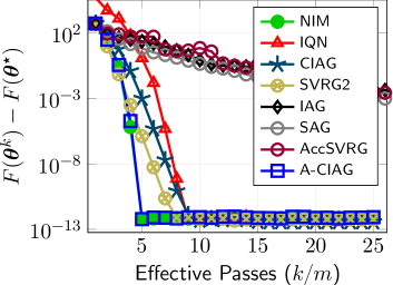
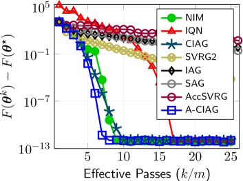
Figure 1: The $y$-axis denotes the optimality gap plotted in log-scale and the $x$-axis shows the number of effective passes (defined as $k/m$). (Left) for the case with $m=1000$, $d=51$. (Right) for the case with $m=2000$, $d=501$. Here, for NIM and SVRG2 we use the step sizes $\gamma=0.01$ and $\gamma=0.1/L$, respectively.

5.1 Synthetic Data

We adopt a simple random data model. First, we generate $\bm{\theta}_{\sf true}\sim{\cal U}[-1,1]^{d}$ and the feature vector as ${\bm{x}}_{i}=[\tilde{\bm{x}}_{i};~{}1]$ where $\tilde{\bm{x}}_{i}\sim{\cal U}[-1,1]^{d-1}$; then, the label is computed as $y_{i}={\rm sign}(\langle{\bm{x}}_{i},\bm{\theta}_{\sf true}\rangle)$.

To set up the benchmark, the step sizes for NIM and IQN are $\gamma=1$. For the IAG method, we set $\gamma=50/(mL)$. For the CIAG and A-CIAG methods, we set $\gamma=1/L$ and we set the extrapolation weight for A-CIAG as $\alpha=0.95$. The above methods are implemented with deterministic, cyclic component function selection, i.e., $i_{k}=(k~{}{\rm mod}~{}m)+1$. We also compare a few stochastic methods: for SAG and AccSVRG, we set $\gamma=50/(mL)$; and the batch size is $B=5$ for AccSVRG with an epoch length of $m$. For SVRG2, we set an epoch length of $0.1m$. The step sizes for NIM and SVRG2 will be specified later.

The evolution of the optimality gap against the number of effective passes through data are shown in Figure 1 for different problem sizes. We defined the number of effective passes as the number of iterations ($k$) divided by $m$. From Figure 1, we observe that both NIM and IQN methods have the fastest convergence, since both methods are shown to converge superlinearly. However, we note that the curvature aided methods, A-CIAG, CIAG and SVRG2, also demonstrate similar convergence speed in terms of the number of effective data passes used. Especially, the speed of the proposed A-CIAG almost matches that of the NIM method.

Dataset	A-CIAG	CIAG	NIM	SAG‡
mushrooms	$\bf 5.22$ pass	$43.5$ pass	$4.81$ ($4.92$) pass	$359.9$ pass
($m=8124,d=112$)	$\bf 0.299$ sec.	$2.509$ sec.	$1.01$ ($0.329$) sec.	$1.521$ sec.
a9a	$\bf 3.6$ pass	$52.2$ pass	$3.0$ ($3.2$) pass	$165.8$ pass
($m=32561,d=123$)	$\bf 1.067$ sec.	$15.26$ sec.	$3.38$ ($1.10$) sec.	$3.685$ sec.
SUSY	$\bf 7.1$ pass	$7.6$ pass	$6.2$ ($6.2$) pass	$52.3$ pass
($m=5\times 10^{6},d=18$)	$\bf 24.88$ sec.	$26.81$ sec.	$35.92$ ($29.82$) sec.	$99.00$ sec.
covtype	$\bf 4.5$ pass	$13.5$ pass	$4.0$ ($4.5$) pass	$101.9$ pass
($m=581012,d=54$)	$\bf 5.888$ sec.	$17.71$ sec.	$13.84$ ($7.06$) sec.	$32.33$ sec.
w8a	$\bf 5.5$ pass	$7.2$ pass	$5.3$ ($5.4$) pass	$251.01$ pass
($m=49749,d=300$)	$\bf 12.73$ sec.	$16.48$ sec.	$69.13$ ($13.82$) sec.	$23.20$ sec.
mnist	$4.3$ pass	$143.6$ pass	$3.8$ ($\bf 3.8$) pass	$\geq 10^{3}$ pass
($m=60000,d=784$)	$89.59$ sec.	$2801$ sec.	$755.2$ ($\bf 86.94$) sec.	$\geq 392$ sec.
alpha	$\bf 2.4$ pass	$7.6$ pass	$2.3$ ($2.5$) pass	$80.5$ pass
($m=5\times 10^{5},d=500$)	$\bf 149.5$ sec.	$475.6$ sec.	$1111.6$ ($176.4$) sec.	210.7 sec.

Table 2: Performance comparison. We show the number of effective passes (defined as $k/m$) and the wall clock time required to reach convergence with $\|{\nabla}F(\bm{\theta}^{k})\|\leq 10^{-10}$. For the NIM method, we tested both ‘exact’ and ‘inexact’ settings in Hessian inverse. Results inside the brackets $(\cdot)$ correspond to ‘inexact’ setting. (^‡Results for SAG are averaged over $10$ trials.)

	mushrooms	a9a	SUSY	covtype	w8a	mnist	alpha
A-CIAG	$\gamma=\frac{10^{-3}}{L}$	$\gamma=\frac{10^{-4}}{L}$	$\gamma=\frac{10^{-5}}{L}$	$\gamma=\frac{5\cdot 10^{-6}}{L}$	$\gamma=\frac{10^{-3}}{L}$	$\gamma=\frac{10^{-4}}{L}$	$\gamma=\frac{5\cdot 10^{-6}}{L}$
	$\alpha=0.99$	$\alpha=0.99$	$\alpha=0.99$	$\alpha=0.99$	$\alpha=0.99$	$\alpha=0.99$	$\alpha=0.99$
CIAG	$\gamma=\frac{10^{-3}}{L}$	$\gamma=\frac{2\cdot 10^{-4}}{L}$	$\gamma=\frac{10^{-5}}{L}$	$\gamma=\frac{5\cdot 10^{-6}}{L}$	$\gamma=\frac{10^{-3}}{L}$	$\gamma=\frac{10^{-4}}{L}$	$\gamma=\frac{10^{-5}}{L}$

Table 3: Parameters used for A-CIAG, CIAG methods in the numerical experiments.

5.2 Real Data

We empirically compare the algorithms on the datasets from LibSVM CC01a . For this example, the algorithms are implemented in C++ based on the source codes by rodomanov2016superlinearly (available: http://github.com/arodomanov/nim_icml16_code) to demonstrate the fastest possible practical performance. We only compare the proposed CIAG, A-CIAG to IAG, NIM and SAG, where the first four algorithms employ a deterministic, cyclic component function selection and the last algorithm employs random component function selection. For the NIM method, we tested both of its exact and inexact setting, where the inexact setting is a double-loop method which uses a conjugate gradient method to tackle the Hessian inverse involved. We have used a mini-batch setting for all the tested methods such that each $f_{i}(\bm{\theta})$ is composed of $B=5$ data tuples. The numerical experiments were conducted on a Laptop computer with an Intel Core i7 2.8Ghz quad-core processor and 16 gigabytes of memory.

An overview of the performance comparison can be found in Table 2, while Table 3 shows the algorithms’ parameter settings used for different dataset. As seen, the A-CIAG method outperformed the benchmarks for many of the considered datasets in terms of the wall clock convergence time, and the number of effective passes required is comparable to the best available method, NIM. An exception is the experiment on the mnist dataset. We suspect that this is due to the potentially poor condition number with the mnist dataset, as we observe that the unaccelerated methods SAG, IAG and CIAG exhibit significantly slower convergence than for the other datasets.

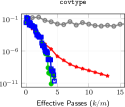
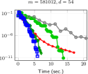
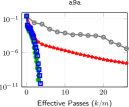
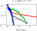
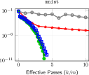
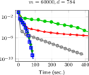
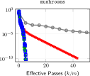
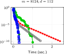
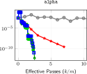
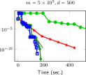
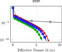
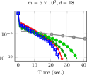
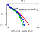
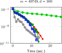
Figure 2: Evolution of $\|{\nabla}F(\bm{\theta}^{k})\|$ ($y$-axis) against number of effective passes and wall clock time on the datasets. The experiment settings are the same as in Table 2.

To investigate the behavior of the algorithms, Figure 2 shows the evolution of gradient’s norm $\|{\nabla}F(\bm{\theta}^{k})\|$ against the number of effective passes and wall clock time on the tested datasets. As seen, the convergence speed of A-CIAG matches that of the Newton-based NIM, yet the wall clock time required is faster as it does not involve computing the Hessians’ inverse. It is worthwhile pointing out that except for the datasets covtype and alpha, the SAG method achieves a solution accuracy of $\|{\nabla}F(\bm{\theta}^{k})\|\leq 10^{-6}$ in less wall clock time than the proposed methods. The benefits of our proposed methods are significant when the solution accuracy is high, as predicted by our theoretical results.

6 Conclusions

We proposed two new optimization methods utilizing curvature-aided gradient tracking for large-scale optimization via incremental data processing. The proposed methods, CIAG and A-CIAG, attain an $\epsilon$-optimal solution with only ${\cal O}({\kappa(F)}\log(1/\epsilon))$ and ${\cal O}(\sqrt{\kappa(F)}\log(1/\epsilon))$ iterations, respectively, for a small $\epsilon$, and provided that the initial point is close to the optimal solution. Numerical experiments on real and synthetic data demonstrate the benefit of our algorithms. Future work includes designing and analyzing an optimal ‘re-starting’ scheme to achieve the ideal convergence rate (37) when the initial point is not close to the optimal solution, and extending the methods to tackling non-smooth optimization problems.

Appendix A Proof of Proposition 3

Let us express the gradient error as ${\bm{e}}_{\sf CIAG}^{k}=\sum_{i=1}^{m}\big{(}{\nabla}f_{i}(\bm{\theta}^{\tau_{i}^{k}})+{\nabla}^{2}f_{i}(\bm{\theta}^{\tau_{i}^{k}})(\bm{\theta}^{k}-\bm{\theta}^{\tau_{i}^{k}})-{\nabla}f_{i}(\bm{\theta}^{k})\big{)}$. Applying Lemma 1:

$$\begin{split}&\|{\bm{e}}_{\sf CIAG}^{k}\|\leq\sum_{i=1}^{m}\frac{L_{H,i}}{2}\|\bm{\theta}^{\tau_{i}^{k}}-\bm{\theta}^{k}\|^{2}\leq\sum_{i=1}^{m}\frac{L_{H,i}}{2}\underbrace{(k-\tau_{i}^{k})}_{\leq K}\sum_{j=\tau_{i}^{k}}^{k-1}\|\bm{\theta}^{j+1}-\bm{\theta}^{j}\|^{2}\\ &\leq\frac{KL_{H}}{2}\sum_{j=(k-K)_{++}}^{k-1}\|\bm{\theta}^{j+1}-\bm{\theta}^{j}\|^{2}\leq\frac{KL_{H}}{2}\gamma^{2}\sum_{j=(k-K)_{++}}^{k-1}\|{\bm{e}}_{\sf CIAG}^{j}+{\nabla}F(\bm{\theta}^{j})\|^{2}\\ &\leq\gamma^{2}KL_{H}\sum_{j=(k-K)_{++}}^{k-1}\big{(}\|{\bm{e}}_{\sf CIAG}^{j}\|^{2}+\|{\nabla}F(\bm{\theta}^{j})\|^{2}\big{)}\;.\end{split}$$ (59)

Furthermore, we have

$$\|{\nabla}F(\bm{\theta}^{j})\|^{2}=\|{\nabla}F(\bm{\theta}^{j})-{\nabla}F(\bm{\theta}^{\star})\|^{2}\leq L^{2}V^{(j)},$$ (60)

$$\begin{split}\|{\bm{e}}_{\sf CIAG}^{j}\|&\overset{(a)}{\leq}\sum_{i=1}^{m}L_{H,i}\big{(}V^{(j)}+V^{(\tau_{i}^{j})}\big{)}\leq 2L_{H}\max_{\ell\in\{\tau_{i}^{j}\}_{i=1}^{m}\cup\{j\}}V^{(\ell)}\;,\end{split}$$ (61)

where (a) is due to $\|{\bm{a}}-{\bm{b}}\|^{2}\leq 2(\|{\bm{a}}\|^{2}+\|{\bm{b}}\|^{2})$. Plugging these back into (59) and using $\tau_{i}^{k-K}\geq k-2K$ gives:

$$\begin{split}\|{\bm{e}}_{\sf CIAG}^{k}\|&\leq\gamma^{2}KL_{H}\sum_{j=(k-K)_{++}}^{k-1}\Big{(}L^{2}V^{(j)}+\big{(}2L_{H}\max_{\ell\in\{\tau_{i}^{j}\}_{i=1}^{m}\cup\{j\}}V^{(\ell)}\big{)}^{2}\Big{)}\\ &\leq\gamma^{2}K^{2}L_{H}\Big{(}L^{2}\max_{(k-K)_{++}\leq\ell\leq k-1}V^{(\ell)}+4L_{H}^{2}\max_{(k-2K)_{++}\leq\ell\leq k-1}(V^{(\ell)})^{2}\Big{)}\;.\end{split}$$ (62)

Appendix B Step 3 in the Proof of Theorem 1

Combining Proposition 1 and 3 yields

$$\begin{split}V^{(k+1)}&\leq\Big{(}1-2\gamma\frac{\mu L}{\mu+L}\Big{)}V^{(k)}\\ &+2\gamma^{3}K^{2}L_{H}\Big{(}L^{2}\max_{(k-K)_{++}\leq\ell\leq k}(V^{(\ell)})^{\frac{3}{2}}+4L_{H}^{2}\max_{(k-2K)_{++}\leq\ell\leq k}(V^{(\ell)})^{\frac{5}{2}}\Big{)}\\ &+2\gamma^{6}K^{4}L_{H}^{2}\Big{(}L^{4}\max_{(k-K)_{++}\leq\ell\leq k-1}(V^{(\ell)})^{2}+16L_{H}^{4}\max_{(k-2K)_{++}\leq\ell\leq k-1}(V^{(\ell)})^{4}\Big{)},\end{split}$$ (63)

which is the exact form for Eq. (44). The right hand side in (63) can be decomposed into two terms — the first term is of the same order as $V^{(k)}$, and the other terms are delayed and higher-order terms of $V^{(\ell)}$.

Observe that (63) is a special case of (48) in Proposition 5 with $R^{(k)}=V^{(k)}$, $M=2K+1$, $p=1-2\gamma\mu L/(\mu+L)$ and

$$\begin{split}&q_{1}=2\gamma^{3}K^{2}L^{2}L_{H},~{}\eta_{1}=3/2,~{}q_{2}=8\gamma^{3}K^{2}L_{H}^{3},~{}\eta_{3}=5/2\;,\\ &q_{3}=2\gamma^{6}K^{4}L_{H}^{2}L^{4},~{}\eta_{3}=2,~{}q_{4}=32\gamma^{6}K^{4}L_{H}^{6},~{}\eta_{4}=4\;.\end{split}$$ (64)

The corresponding convergence condition in (49) can be satisfied if

$$\begin{split}&\gamma^{5}\!~{}2K^{4}L_{H}^{2}\Big{(}L^{4}V^{(1)}+16L_{H}^{4}(V^{(1)})^{3}\Big{)}<\frac{\mu L}{\mu+L}\\ &\text{and}~{}~{}\gamma^{2}\!~{}2K^{2}L_{H}\Big{(}L^{2}(V^{(1)})^{1/2}+4L_{H}^{2}(V^{(1)})^{3/2}\Big{)}<\frac{\mu L}{\mu+L}\;,\end{split}$$ (65)

which can be implied by (28). The proof is thus concluded.

Appendix C Proof of Proposition 5

The proof of the proposition is divided into two parts. We first show that under (49), the sequence $\{R^{(k)}\}_{k\geq 1}$ converges linearly as in part (a) of the proposition; then we show that the rate of convergence is asymptotically given by $p$ as in part (b) of the proposition [cf. (50)].

The first part of the proof is achieved using induction on all $\ell\geq 1$ with:

$$R^{(k)}\leq\delta^{\ell}\!~{}R^{(1)},~{}\forall~{}k=(\ell-1)M+2,...,\ell M+1\;.$$ (66)

The base case when $\ell=1$ can be straightforwardly established:

$$\begin{split}&\textstyle R^{(2)}\leq pR^{(1)}+\sum_{j=1}^{J}q_{j}(R^{(1)})^{\eta_{j}}\leq\delta R^{(1)}\;,\\ &\vdots\\ &\textstyle R^{(M+1)}\leq pR^{(M)}+\sum_{j=1}^{J}q_{j}(R^{(0)})^{\eta_{j}}\leq\delta R^{(1)}\;.\end{split}$$ (67)

Suppose that the statement (66) is true up to $\ell=c$, for $\ell=c+1$, we have:

$$\begin{split}R^{(cM+2)}&\leq pR^{(cM+1)}+\sum_{j=1}^{J}q_{j}\max_{k^{\prime}\in[(c-1)M+2,cM+1]}(R^{(k^{\prime})})^{\eta_{j}}\\ &\leq p\big{(}\delta^{c}R^{(1)}\big{)}+\sum_{j=1}^{J}q_{j}\big{(}\delta^{c}R^{(1)}\big{)}^{\eta_{j}}\leq\delta^{c}\!~{}\Big{(}pR^{(1)}+\sum_{j=1}^{J}q_{j}(R^{(1)})^{\eta_{j}}\Big{)}\leq\delta^{c+1}R^{(1)}\;.\end{split}$$

Similar statement also holds for $R^{(k)}$ with $k=cM+3,...,(c+1)M+1$. We thus conclude with:

$$R^{(k)}\leq\delta^{\lceil(k-1)/M\rceil}\!~{}R^{(1)},~{}\forall~{}k\geq 1\;,$$ (68)

which proves the first part of the proposition.

The second part of the proof establishes the asymptotic linear rate of convergence in (50). We consider the upper bound sequence $\{\bar{R}^{(k)}\}_{k\geq 1}$ such that $\bar{R}^{(1)}=R^{(1)}$ and the inequality (48) is tight for $\{\bar{R}^{(k)}\}_{k\geq 1}$. Obviously, it also holds that $\bar{R}^{(k)}\leq\delta^{\lceil(k-1)/M\rceil}\bar{R}^{(1)}$ for all $k\geq 1$. Now, observe that

$$\frac{\bar{R}^{(k+1)}}{\bar{R}^{(k)}}=p+\frac{\sum_{j=1}^{J}q_{j}\max_{k^{\prime}\in[(k-M+1)_{++},k]}(R^{(k^{\prime})})^{\eta_{j}}}{\bar{R}^{(k)}}\;.$$ (69)

For any $k^{\prime}\in[k-M+1,k]$ and any $\eta>1$, we have:

$$\begin{split}&\frac{(\bar{R}^{(k^{\prime})})^{\eta}}{\bar{R}^{(k)}}=\frac{\bar{R}^{(k^{\prime})}}{\bar{R}^{(k)}}\!~{}(\bar{R}^{(k^{\prime})})^{\eta-1}\leq\frac{\bar{R}^{(k^{\prime})}}{\bar{R}^{(k)}}(R^{(1)})^{\eta-1}\delta^{(\lceil\frac{k^{\prime}-1}{M}\rceil)(\eta-1)}\;.\end{split}$$ (70)

Note that as $\bar{R}^{(k+1)}/\bar{R}^{(k)}\geq p$, we have:

$$\frac{(\bar{R}^{(k^{\prime})})^{\eta}}{\bar{R}^{(k)}}\leq p^{-M}(R^{(1)})^{\eta-1}\delta^{(\lceil\frac{k^{\prime}-1}{M}\rceil)(\eta-1)}\;.$$ (71)

Taking $k\rightarrow\infty$ shows that the right hand side vanishes. As a result, we have $\lim_{k\rightarrow\infty}\bar{R}^{(k+1)}/\bar{R}^{(k)}=p$. This proves part (b) of the proposition.

Appendix D Proof of Proposition 2

The following proof is partially inspired by schmidt2011convergence ; bubeck2015convex ; nitanda2014stochastic . For simplicity, we drop the subscript ACIAG in ${\bm{g}}_{\sf ACIAG}^{k}$ and ${\bm{e}}_{\sf ACIAG}^{k}$. Define $\rho\mathrel{\mathop{:}}=1-\sqrt{\mu\gamma}$ and the estimation sequence as:

$$\begin{split}\Phi_{1}(\bm{\theta})&\mathrel{\mathop{:}}=F(\bm{\theta}_{ex}^{1})+\frac{\mu}{2}\|\bm{\theta}-\bm{\theta}_{ex}^{1}\|^{2}\\ \Phi_{k+1}(\bm{\theta})&\mathrel{\mathop{:}}=\rho\!~{}\Phi_{k}(\bm{\theta})+\sqrt{\mu\gamma}\Big{(}F(\bm{\theta}_{ex}^{k})+\langle{\bm{g}}^{k},\bm{\theta}-\bm{\theta}_{ex}^{k}\rangle+\frac{\mu}{2}\|\bm{\theta}-\bm{\theta}_{ex}^{k}\|^{2}\Big{)}\;,\end{split}$$ (72)

where ${\bm{g}}^{k}\mathrel{\mathop{:}}={\bm{b}}^{k}+{\bm{H}}^{k}\bm{\theta}_{ex}^{k}$ is the gradient surrogate used in (17). Recall that ${\bm{e}}^{k}\mathrel{\mathop{:}}={\bm{g}}^{k}-{\nabla}F(\bm{\theta}_{ex}^{k})$ is the gradient error. The following inequality, which holds for all $\bm{\theta}\in\mathbb{R}^{d}$, can be immediately obtained using (72) and the $\mu$-strong convexity of $F(\bm{\theta})$:

$$\begin{split}&\Phi_{k+1}(\bm{\theta})-F(\bm{\theta})=\rho\Phi_{k}(\bm{\theta})-F(\bm{\theta})\\ &\hskip 42.67912pt+\sqrt{\mu\gamma}\Big{(}F(\bm{\theta}_{ex}^{k})+\langle{\nabla}F(\bm{\theta}_{ex}^{k})+{\bm{e}}^{k},\bm{\theta}-\bm{\theta}_{ex}^{k}\rangle+\frac{\mu}{2}\|\bm{\theta}-\bm{\theta}_{ex}^{k}\|^{2}\Big{)}\\ &\leq\rho\big{(}\Phi_{k}(\bm{\theta})-F(\bm{\theta})\big{)}+\sqrt{\mu\gamma}\langle{\bm{e}}^{k},\bm{\theta}-\bm{\theta}_{ex}^{s}\rangle\\ &\leq\rho^{k}\big{(}\Phi_{1}(\bm{\theta})-F(\bm{\theta})\big{)}+\sum_{\ell=1}^{k}\rho^{k-\ell}\sqrt{\mu\gamma}\langle{\bm{e}}^{\ell},\bm{\theta}-\bm{\theta}_{ex}^{\ell}\rangle\;.\end{split}$$ (73)

To facilitate our development, let us denote:

$$\Phi_{k}^{\star}\mathrel{\mathop{:}}=\min_{\bm{\theta}}\Phi_{k}(\bm{\theta}),~{}~{}{\bm{v}}^{k}\mathrel{\mathop{:}}=\arg\min_{\bm{\theta}}\Phi_{k}(\bm{\theta})\;.$$ (74)

By setting $\bm{\theta}=\bm{\theta}^{\star}$ in (73), we have:

$$\begin{split}&\Phi_{k+1}^{\star}-F(\bm{\theta}^{\star})\leq\Phi_{k+1}(\bm{\theta}^{\star})-F(\bm{\theta}^{\star})\\ &\leq\rho^{k}\Big{(}\frac{\mu}{2}\|\bm{\theta}^{\star}-\bm{\theta}_{ex}^{1}\|^{2}+F(\bm{\theta}_{ex}^{1})-F(\bm{\theta}^{\star})\Big{)}+\sum_{\ell=1}^{k}\rho^{k-\ell}\sqrt{\mu\gamma}\langle{\bm{e}}^{\ell},\bm{\theta}^{\star}-\bm{\theta}_{ex}^{\ell}\rangle\\ &\leq 2\rho^{k}\Big{(}F(\bm{\theta}^{1})-F(\bm{\theta}^{\star})\Big{)}+\sum_{\ell=1}^{k}\rho^{k-\ell}\sqrt{\mu\gamma}\langle{\bm{e}}^{\ell},\bm{\theta}^{\star}-\bm{\theta}_{ex}^{\ell}\rangle\;.\end{split}$$ (75)

Now, if $F(\bm{\theta}^{k+1})\leq\Phi_{k+1}^{\star}$, then the inequality above shows the evolution of the optimality gap $h^{(k)}$. This motivates our next step, relating $F(\bm{\theta}^{k+1})$ to $\Phi_{k+1}^{\star}$.

Lower bounding $\Phi_{k+1}^{\star}$ in the presence of errors. Since ${\nabla}^{2}\Phi_{k}(\bm{\theta})=\mu{\bm{I}}$, the function $\Phi_{k}(\bm{\theta})$ is quadratic and we can represent $\Phi_{k}(\bm{\theta})$ alternatively as

$$\Phi_{k}(\bm{\theta})=\Phi_{k}^{\star}+\frac{\mu}{2}\|\bm{\theta}-{\bm{v}}^{k}\|^{2}\;.$$ (76)

By substituting (76) into the definition of $\Phi_{k+1}(\bm{\theta})$ in (72) and evaluating the first order optimality condition of the latter, we have:

$$\begin{split}&\sqrt{\mu\gamma}({\bm{g}}^{k}+\mu({\bm{v}}^{k+1}-\bm{\theta}_{ex}^{k}))+\rho\!~{}\mu({\bm{v}}^{k+1}-{\bm{v}}^{k})={\bm{0}}\;,\\ &\Longrightarrow{\bm{v}}^{k+1}=\rho{\bm{v}}^{k}+\sqrt{\mu\gamma}\bm{\theta}_{ex}^{k}-\sqrt{\frac{\gamma}{\mu}}{\bm{g}}^{k}\;.\end{split}$$ (77)

By setting $\bm{\theta}=\bm{\theta}_{ex}^{k}$ in (72) and using the recursive definition of $\Phi_{k+1}(\bm{\theta})$, we obtain

$$\begin{split}\Phi_{k+1}(\bm{\theta}_{ex}^{k})&=\rho\Phi_{k}(\bm{\theta}_{ex}^{k})+\sqrt{\mu\gamma}F(\bm{\theta}_{ex}^{k})=\rho\big{(}\Phi_{k}^{\star}+\frac{\mu}{2}\|\bm{\theta}_{ex}^{k}-{\bm{v}}^{k}\|^{2}\big{)}+\sqrt{\mu\gamma}F(\bm{\theta}_{ex}^{k})\;,\end{split}$$ (78)

while setting $\bm{\theta}=\bm{\theta}_{ex}^{k}$ in (76) and using (77) gives us:

$$\begin{split}\Phi_{k+1}(\bm{\theta}_{ex}^{k})&=\Phi_{k+1}^{\star}+\frac{\mu}{2}\Big{(}\rho^{2}\|\bm{\theta}_{ex}^{k}-{\bm{v}}^{k}\|^{2}+\frac{\gamma}{\mu}\|{\bm{g}}^{k}\|^{2}+2\rho\sqrt{\frac{\gamma}{\mu}}\langle{\bm{g}}^{k},\bm{\theta}_{ex}^{k}-{\bm{v}}^{k}\rangle\Big{)}\;.\end{split}$$ (79)

Comparing the right hand side of (78) and (79) shows:

$$\begin{split}\Phi_{k+1}^{\star}&=\rho\Big{(}\Phi_{k}^{\star}+\frac{\mu}{2}\|\bm{\theta}_{ex}^{k}-{\bm{v}}^{k}\|^{2}\Big{)}+\sqrt{\mu\gamma}F(\bm{\theta}_{ex}^{k})\\ &~{}~{}~{}-\frac{\mu}{2}\Big{(}\rho^{2}\|\bm{\theta}_{ex}^{k}-{\bm{v}}^{k}\|^{2}+\frac{\gamma}{\mu}\|{\bm{g}}^{k}\|^{2}+2\rho\sqrt{\frac{\gamma}{\mu}}\langle{\bm{g}}^{k},\bm{\theta}_{ex}^{k}-{\bm{v}}^{k}\rangle\Big{)}\\ &=\rho\Phi_{k}^{\star}+\sqrt{\mu\gamma}F(\bm{\theta}_{ex}^{k})+\frac{\mu}{2}\rho\sqrt{\mu\gamma}\|\bm{\theta}_{ex}^{k}-{\bm{v}}^{k}\|^{2}-\frac{\gamma}{2}\|{\bm{g}}^{k}\|^{2}-\rho\sqrt{\mu\gamma}\langle{\bm{g}}^{k},\bm{\theta}_{ex}^{k}-{\bm{v}}^{k}\rangle\;.\end{split}$$

Using the fact ${\bm{v}}^{k}-\bm{\theta}_{ex}^{k}=(\sqrt{\mu\gamma})^{-1}\big{(}\bm{\theta}_{ex}^{k}-\bm{\theta}^{k}\big{)}$ (proven in Section D.1), we have

$$\begin{split}\Phi_{k+1}^{\star}&=\rho\Phi_{k}^{\star}+\sqrt{\mu\gamma}F(\bm{\theta}_{ex}^{k})+\frac{\mu}{2}\frac{\rho}{\sqrt{\mu\gamma}}\|\bm{\theta}_{ex}^{k}-\bm{\theta}^{k}\|^{2}-\frac{\gamma}{2}\|{\bm{g}}^{k}\|^{2}-\rho\langle{\bm{g}}^{k},\bm{\theta}^{k}-\bm{\theta}_{ex}^{k}\rangle\;.\end{split}$$ (80)

We obtain the following chain:

$$\begin{split}&F(\bm{\theta}^{k+1})-\Phi_{k+1}^{\star}\overset{(a)}{\leq}F(\bm{\theta}_{ex}^{k})-\gamma\langle{\nabla}F(\bm{\theta}_{ex}^{k}),{\bm{g}}^{k}\rangle+\frac{L\gamma^{2}}{2}\|{\bm{g}}^{k}\|^{2}-\Phi_{k+1}^{\star}\\ &\overset{(b)}{=}\rho\!~{}\Big{(}F(\bm{\theta}_{ex}^{k})+\langle{\bm{g}}^{k},\bm{\theta}^{k}-\bm{\theta}_{ex}^{k}\rangle-\Phi_{k}^{\star}\Big{)}\\ &\hskip 14.22636pt-\gamma\langle{\nabla}F(\bm{\theta}_{ex}^{k}),{\bm{g}}^{k}\rangle+\frac{\gamma}{2}\Big{(}1+L\gamma\Big{)}\|{\bm{g}}^{k}\|^{2}-\frac{\mu}{2}\frac{\rho}{\sqrt{\mu\gamma}}\|\bm{\theta}_{ex}^{k}-\bm{\theta}^{k}\|^{2}\\ &\overset{(c)}{=}\rho\!~{}\big{(}F(\bm{\theta}_{ex}^{k})+\langle{\nabla}F(\bm{\theta}_{ex}^{k}),\bm{\theta}^{k}-\bm{\theta}_{ex}^{k}\rangle-\Phi_{k}^{\star}\big{)}-\gamma\langle{\nabla}F(\bm{\theta}_{ex}^{k}),{\bm{g}}^{k}\rangle\\ &\hskip 14.22636pt+\rho\langle{\bm{e}}^{k},\bm{\theta}^{k}-\bm{\theta}_{ex}^{k}\rangle+\frac{\gamma}{2}\Big{(}1+L\gamma\Big{)}\|{\bm{g}}^{k}\|^{2}-\frac{\mu}{2}\frac{\rho}{\sqrt{\mu\gamma}}\|\bm{\theta}_{ex}^{k}-\bm{\theta}^{k}\|^{2}\\ &\overset{(d)}{\leq}\rho\!~{}\big{(}F(\bm{\theta}^{k})-\Phi_{k}^{\star}+\langle{\bm{e}}^{k},\bm{\theta}^{k}-\bm{\theta}_{ex}^{k}\rangle\big{)}-\frac{\mu}{2}\frac{1-\mu\gamma}{\sqrt{\mu\gamma}}\|\bm{\theta}_{ex}^{k}-\bm{\theta}^{k}\|^{2}\\ &\hskip 14.22636pt+\frac{\gamma}{2}\Big{(}1+L\gamma\Big{)}\|{\bm{g}}^{k}\|^{2}-\gamma\langle{\nabla}F(\bm{\theta}_{ex}^{k}),{\bm{g}}^{k}\rangle\\ &\overset{(e)}{\leq}\rho\!~{}\big{(}F(\bm{\theta}^{k})-\Phi_{k}^{\star}+\langle{\bm{e}}^{k},\bm{\theta}^{k}-\bm{\theta}_{ex}^{k}\rangle\big{)}-\frac{\mu}{2}\frac{1-\mu\gamma}{\sqrt{\mu\gamma}}\|\bm{\theta}_{ex}^{k}-\bm{\theta}^{k}\|^{2}+\gamma\|{\bm{e}}^{k}\|^{2}\;,\end{split}$$ (81)

where (a) is due to the $L$-smoothness of $F$; (b) is due to (80); (c) is obtained by expanding ${\bm{g}}^{k}$ as ${\nabla}F(\bm{\theta}_{ex}^{k})+{\bm{e}}^{k}$; (d) is obtained by adding and subtracting $(\mu/2)\|\bm{\theta}^{k}-\bm{\theta}_{ex}^{k}\|^{2}$ inside the first bracket, applying the identity $\rho+\rho/\sqrt{\mu\gamma}=(1-\mu\gamma)/\sqrt{\mu\gamma}$, and using the $\mu$-strong convexity of $F$; and (e) is due to the following chain of inequalities:

$$\begin{split}&\frac{\gamma}{2}\Big{(}1+L\gamma\Big{)}\|{\bm{g}}^{k}\|^{2}-\gamma\langle{\nabla}F(\bm{\theta}_{ex}^{k}),{\bm{g}}^{s}\rangle\\ &\leq\frac{\gamma}{2}\Big{(}1+L\gamma\Big{)}\Big{(}\|{\bm{e}}^{k}\|^{2}+\|{\nabla}F(\bm{\theta}_{ex}^{k})\|^{2}\Big{)}+\frac{L\gamma^{2}}{2}\Big{(}\|{\nabla}F(\bm{\theta}_{ex}^{k})\|^{2}+\|{\bm{e}}^{k}\|^{2}\Big{)}-\gamma\|{\nabla}F(\bm{\theta}_{ex}^{k})\|^{2}\\ &=\Big{(}\frac{\gamma}{2}+L\gamma^{2}\Big{)}\|{\bm{e}}^{k}\|^{2}+\Big{(}-\frac{\gamma}{2}+L\gamma^{2}\Big{)}\|{\nabla}F(\bm{\theta}_{ex}^{k})\|^{2}\leq\gamma\|{\bm{e}}^{k}\|^{2}\;.\end{split}$$

As $\Phi_{1}(\bm{\theta}^{1})=F(\bm{\theta}^{1})=\Phi_{1}^{\star}$, applying the inequality (81) recursively shows:

$$\begin{split}&F(\bm{\theta}^{k+1})-\Phi_{k+1}^{\star}\leq\\ &\sum_{\ell=1}^{k}\rho^{k-\ell}\Big{(}(1-\sqrt{\mu\gamma})\langle{\bm{e}}^{\ell},\bm{\theta}^{\ell}-\bm{\theta}_{ex}^{\ell}\rangle+\gamma\|{\bm{e}}^{\ell}\|^{2}-\frac{\mu}{2}\frac{1-\mu\gamma}{\sqrt{\mu\gamma}}\|\bm{\theta}_{ex}^{\ell}-\bm{\theta}^{\ell}\|^{2}\Big{)}\;.\end{split}$$ (82)

Importantly, (82) establishes a lower bound on $\Phi_{k+1}^{\star}$ in terms of $F(\bm{\theta}^{k+1})$ and ${\bm{e}}^{k}$.

Proving Proposition 2. Finally, summing up (82) and (75) gives:

$$\begin{split}h^{(k+1)}&\leq 2\rho^{k}h^{(1)}+\sum_{\ell=1}^{k}\rho^{k-\ell}\Big{(}\sqrt{\mu\gamma}\langle{\bm{e}}^{\ell},\bm{\theta}^{\star}-\bm{\theta}_{ex}^{\ell}\rangle\\ &\hskip 42.67912pt+\rho\langle{\bm{e}}^{\ell},\bm{\theta}^{\ell}-\bm{\theta}_{ex}^{\ell}\rangle+\gamma\|{\bm{e}}^{\ell}\|^{2}-\frac{\mu}{2}\frac{1-\mu\gamma}{\sqrt{\mu\gamma}}\|\bm{\theta}_{ex}^{\ell}-\bm{\theta}^{\ell}\|^{2}\Big{)}\\ &=2\rho^{k}h^{(1)}+\sum_{\ell=1}^{k}\rho^{k-\ell}\Big{(}\sqrt{\mu\gamma}\langle{\bm{e}}^{\ell},\bm{\theta}^{\star}-\bm{\theta}^{\ell}\rangle\\ &\hskip 42.67912pt+\langle{\bm{e}}^{\ell},\bm{\theta}^{\ell}-\bm{\theta}_{ex}^{\ell}\rangle+\gamma\|{\bm{e}}^{\ell}\|^{2}-\frac{\mu}{2}\frac{1-\mu\gamma}{\sqrt{\mu\gamma}}\|\bm{\theta}_{ex}^{\ell}-\bm{\theta}^{\ell}\|^{2}\Big{)}\;.\end{split}$$ (83)

Let us take a look at the last summands in the above inequality: for any $\ell\geq 1$,

$$\begin{split}&\sqrt{\mu\gamma}\langle{\bm{e}}^{\ell},\bm{\theta}^{\star}-\bm{\theta}^{\ell}\rangle+\langle{\bm{e}}^{\ell},\bm{\theta}^{\ell}-\bm{\theta}_{ex}^{\ell}\rangle+\gamma\|{\bm{e}}^{\ell}\|^{2}-\frac{\mu}{2}\frac{1-\mu\gamma}{\sqrt{\mu\gamma}}\|\bm{\theta}_{ex}^{\ell}-\bm{\theta}^{\ell}\|^{2}\\ &\overset{(a)}{\leq}\sqrt{\mu\gamma}\|{\bm{e}}^{\ell}\|\|\bm{\theta}^{\star}-\bm{\theta}^{\ell}\|+\Big{(}\gamma+\frac{\sqrt{\gamma/\mu}}{1-\mu\gamma}\Big{)}\|{\bm{e}}^{\ell}\|^{2}-\frac{\mu}{4}\frac{1-\mu\gamma}{\sqrt{\mu\gamma}}\|\bm{\theta}_{ex}^{\ell}-\bm{\theta}^{\ell}\|^{2}\\ &\overset{(b)}{\leq}\sqrt{2\gamma h^{(\ell)}}\|{\bm{e}}^{\ell}\|+\Big{(}\gamma+\frac{\sqrt{\gamma/\mu}}{1-\mu\gamma}\Big{)}\|{\bm{e}}^{\ell}\|^{2}-\frac{\mu}{4}\frac{1-\mu\gamma}{\sqrt{\mu\gamma}}\|\bm{\theta}_{ex}^{\ell}-\bm{\theta}^{\ell}\|^{2}\\ &\overset{(c)}{\leq}\sqrt{2\gamma h^{(\ell)}}\|{\bm{e}}^{\ell}\|+\sqrt{\frac{9\gamma}{\mu}}\|{\bm{e}}^{\ell}\|^{2}-\frac{\mu}{4}\frac{1-\mu\gamma}{\sqrt{\mu\gamma}}\|\bm{\theta}_{ex}^{\ell}-\bm{\theta}^{\ell}\|^{2}\;,\end{split}$$ (84)

where (a) is resulted from the fact $\langle{\bm{e}}^{\ell},\bm{\theta}^{\ell}-\bm{\theta}_{ex}^{\ell}\rangle\leq(1/2)(\|{\bm{e}}^{\ell}\|^{2}/c+c\|\bm{\theta}^{\ell}-\bm{\theta}_{ex}^{\ell}\|^{2})$ for any $c>0$ and we have set $c=\frac{\mu}{2}\frac{1-\mu\gamma}{\sqrt{\mu\gamma}}$ therein; (b) is due to the relation $\|\bm{\theta}^{\ell}-\bm{\theta}^{\star}\|\leq\sqrt{2h^{(\ell)}/\mu}$; (c) is due to $\gamma+\frac{\sqrt{\gamma/\mu}}{1-\mu\gamma}\leq 3\sqrt{\gamma/\mu}$, which can be verified through replacing $\gamma$ by its upper bound $1/(2L)$ in the denominator of the fraction on the left-hand-side. Combining the two equations above yields the desired result of Proposition.

D.1 Proof of the Equality

We prove ${\bm{v}}^{k}-\bm{\theta}_{ex}^{k}=(\sqrt{\mu\gamma})^{-1}\big{(}\bm{\theta}_{ex}^{k}-\bm{\theta}^{k}\big{)}$ using induction on $k$. Clearly, the said equality holds for $k=1$ since ${\bm{v}}^{1}=\bm{\theta}^{1}=\bm{\theta}_{ex}^{1}$, and we assume that it holds up to $k$. Consider:

$$\begin{split}&{\bm{v}}^{k+1}-\bm{\theta}_{ex}^{k+1}=\rho{\bm{v}}^{k}+\sqrt{\mu\gamma}\bm{\theta}_{ex}^{k}-\sqrt{\frac{\gamma}{\mu}}{\bm{g}}^{k}-\bm{\theta}_{ex}^{k+1}\\ &=\rho({\bm{v}}^{k}-\bm{\theta}_{ex}^{k})+\bm{\theta}_{ex}^{k}-\sqrt{\frac{\gamma}{\mu}}{\bm{g}}^{k}-\bm{\theta}_{ex}^{k+1}=\frac{\rho}{\sqrt{\mu\gamma}}(\bm{\theta}_{ex}^{k}-\bm{\theta}^{k})+\bm{\theta}_{ex}^{k}-\sqrt{\frac{\gamma}{\mu}}{\bm{g}}^{k}-\bm{\theta}_{ex}^{k+1}\;,\end{split}$$

where we have used the induction hypothesis. Furthermore, using $\bm{\theta}^{k+1}=\bm{\theta}_{ex}^{k}-\gamma{\bm{g}}^{k}$,

$$\begin{split}&{\bm{v}}^{k+1}-\bm{\theta}_{ex}^{k+1}=\sqrt{\mu\gamma}^{-1}\Big{(}\rho(\bm{\theta}_{ex}^{k}-\bm{\theta}^{k})+\sqrt{\mu\gamma}(\bm{\theta}_{ex}^{k}-\bm{\theta}_{ex}^{k+1})-\gamma{\bm{g}}^{k}\Big{)}\\ &\overset{(a)}{=}\sqrt{\mu\gamma}^{-1}\Big{(}\sqrt{\mu\gamma}(\bm{\theta}^{k+1}-\bm{\theta}_{ex}^{k+1})+\rho(\bm{\theta}^{k+1}-\bm{\theta}^{k})\Big{)}=\sqrt{\mu\gamma}^{-1}\big{(}\bm{\theta}_{ex}^{k+1}-\bm{\theta}^{k+1}\big{)}\;,\end{split}$$ (85)

where (a) is due to $\rho(\bm{\theta}^{k+1}-\bm{\theta}^{k})=(1+\sqrt{\mu\gamma})(\bm{\theta}_{ex}^{k+1}-\bm{\theta}^{k+1})$.

Appendix E Proof of Proposition 4

We begin by observing that due to the $L_{H,i}$-Lipschitz continuity of the Hessian of $f_{i}$ and using Lemma 1, we have:

$$\begin{split}&\|{\bm{e}}_{\sf ACIAG}^{\ell}\|=\|{\bm{g}}_{\sf ACIAG}^{\ell}-{\nabla}F(\bm{\theta}_{ex}^{\ell})\|\leq\sum_{i=1}^{m}\frac{L_{H,i}}{2}\|\bm{\theta}_{ex}^{\ell}-\bm{\theta}_{ex}^{\tau_{i}^{\ell}}\|^{2}\;.\end{split}$$ (86)

Now, expanding the right hand side of (86) gives:

$$\begin{split}\|{\bm{e}}_{\sf ACIAG}^{\ell}\|&\leq\sum_{i=1}^{m}\frac{L_{H,i}}{2}\Big{\|}\bm{\theta}_{ex}^{\ell}-\bm{\theta}_{ex}^{\tau_{i}^{\ell}}\Big{\|}^{2}\leq\sum_{i=1}^{m}\frac{L_{H,i}}{2}\!~{}\underbrace{(\ell-\tau_{i}^{\ell})}_{\leq K}\sum_{j=\ell-\tau_{i}^{\ell}}^{\ell-1}\|\bm{\theta}_{ex}^{j+1}-\bm{\theta}_{ex}^{j}\|^{2}\\ &\leq\frac{KL_{H}}{2}\sum_{j=(\ell-K)_{++}}^{\ell-1}\|\bm{\theta}_{ex}^{j+1}-\bm{\theta}_{ex}^{j}\|^{2}=\frac{KL_{H}}{2}\sum_{j=(\ell-K)_{++}}^{\ell-1}\|\gamma{\bm{g}}_{\sf ACIAG}^{j}+\underbrace{\alpha(\bm{\theta}^{j+1}-\bm{\theta}^{j})}_{=\bm{\theta}_{ex}^{j+1}-\bm{\theta}^{j+1}}\|^{2}\\ &\leq\frac{3KL_{H}}{2}\sum_{j=(\ell-K)_{++}}^{\ell-1}\Big{(}\gamma^{2}\big{(}\|{\bm{e}}^{j}\|^{2}+\|{\nabla}F(\bm{\theta}_{ex}^{j})\|^{2}\big{)}+\|\bm{\theta}_{ex}^{j+1}-\bm{\theta}^{j+1}\|^{2}\Big{)}\;.\end{split}$$ (87)

Remarkably, the above bound resembles that of Proposition 3 with the exception of the last term that depends on $\bm{\theta}_{ex}^{j+1}-\bm{\theta}^{j+1}$. This is included to account for the extrapolated iterates used in the A-CIAG method.

To find an upper bound of $\|{\bm{e}}_{\sf ACIAG}^{\ell}\|$ to corroborate Proposition 4, in what follows, we will upper bound $\|{\bm{e}}_{\sf ACIAG}^{j}\|^{2}$ and $\|{\nabla}F(\bm{\theta}_{ex}^{j})\|^{2}$, respectively. Firstly,

$$\begin{split}\|{\bm{e}}_{\sf ACIAG}^{j}\|&\leq\sum_{i=1}^{m}\frac{L_{H,i}}{2}\Big{\|}\bm{\theta}_{ex}^{j}-\bm{\theta}_{ex}^{\tau_{i}^{j}}\Big{\|}^{2}\\ &\leq\sum_{i=1}^{m}L_{H,i}\Big{(}(1+\alpha)^{2}\|\bm{\theta}^{j}-\bm{\theta}^{\tau_{i}^{j}}\|^{2}+\alpha^{2}\|\bm{\theta}^{j-1}-\bm{\theta}^{\tau_{i}^{j}-1}\|^{2}\Big{)}\;.\end{split}$$ (88)

Noticing that as $\|\bm{\theta}^{j}-\bm{\theta}^{\tau_{i}^{j}}\|^{2}\leq 2(\|\bm{\theta}^{j}-\bm{\theta}^{\star}\|^{2}+\|\bm{\theta}^{\tau_{i}^{j}}-\bm{\theta}^{\star}\|^{2})\leq(4/\mu)(h^{(j)}+h^{(\tau_{i}^{j})})$, it follows from (88) that

$$\begin{split}\|{\bm{e}}_{\sf ACIAG}^{j}\|&\leq\frac{4}{\mu}\sum_{i=1}^{m}L_{H,i}\Big{(}(1+\alpha)^{2}(h^{(j)}+h^{(\tau_{i}^{j})})+\alpha^{2}(h^{(j-1)}+h^{(\tau_{i}^{j}-1)})\Big{)}\\ &\leq\frac{8L_{H}}{\mu}\big{(}(1+\alpha)^{2}+\alpha^{2}\big{)}\max_{(j-K-1)_{++}\leq q\leq j}h^{(q)}\leq\frac{40L_{H}}{\mu}\max_{(j-K-1)_{++}\leq q\leq j}h^{(q)}\;,\end{split}$$ (89)

which implies

$$\begin{split}\sum_{j=(\ell-K)_{++}}^{\ell-1}\|{\bm{e}}_{\sf ACIAG}^{j}\|^{2}&\leq K\Big{(}\frac{40L_{H}}{\mu}\Big{)}^{2}\max_{(\ell-2K-1)_{++}\leq q\leq\ell}(h^{(q)})^{2}\;.\end{split}$$ (90)

Secondly,

$$\begin{split}\|{\nabla}F(\bm{\theta}_{ex}^{j})\|^{2}&\leq 2L^{2}\big{(}\|\bm{\theta}^{j}-\bm{\theta}^{\star}\|^{2}+\|\bm{\theta}^{j}-\bm{\theta}^{j-1}\|^{2}\big{)}\leq\frac{4L^{2}}{\mu}\Big{(}3h^{(j)}+2h^{(j-1)})\Big{)}\;,\end{split}$$ (91)

thus

$$\begin{split}\sum_{j=(\ell-K)_{++}}^{\ell-1}\|{\nabla}F(\bm{\theta}_{ex}^{j})\|^{2}&\leq\frac{20L^{2}K}{\mu}\max_{(\ell-K-1)_{++}\leq q\leq\ell-1}h^{(q)}\;.\end{split}$$ (92)

Substituting (90) and (92) into the right hand side of (87) verifies Proposition 4.

Appendix F Step 3 in the Proof of Theorem 2

To proceed with the proof, let us define the following quantity:

$$\begin{split}&\tilde{E}^{(\ell)}\mathrel{\mathop{:}}=\gamma^{\frac{5}{2}}\sqrt{\frac{9}{2}}K^{2}L_{H}\Big{(}\big{(}\frac{40L_{H}}{\mu}\big{)}^{2}\max_{(\ell-2K-1)_{++}\leq q\leq\ell}(h^{(q)})^{2}+\frac{20L^{2}}{\mu}\max_{(\ell-K-1)_{++}\leq q\leq\ell}h^{(q)}\Big{)}\\ &+\gamma^{\frac{9}{2}}\frac{81K^{4}L_{H}^{2}}{4\sqrt{\mu}}\Big{(}\big{(}\frac{40L_{H}}{\mu}\big{)}^{4}\max_{(\ell-2K-1)_{++}\leq q\leq\ell}(h^{(q)})^{4}+\big{(}\frac{20L^{2}}{\mu}\big{)}^{2}\max_{(\ell-K-1)_{++}\leq q\leq\ell}(h^{(q)})^{2}\Big{)}\;.\end{split}$$

Using Proposition 4, we obtain:

$$\begin{split}&\sqrt{2\gamma h^{(\ell)}}\|{\bm{e}}_{\sf ACIAG}^{\ell}\|+\sqrt{\frac{9\gamma}{\mu}}\|{\bm{e}}_{\sf ACIAG}^{\ell}\|^{2}\\ &\leq\tilde{E}^{(\ell)}+\sum_{j=(\ell-K+1)_{++}}^{\ell}\Big{(}\sqrt{\frac{9\gamma h^{(\ell)}K^{2}L_{H}^{2}}{2}}\|\bm{\theta}^{j}-\bm{\theta}_{ex}^{j}\|^{2}+\frac{27K^{3}L_{H}^{2}}{4}\sqrt{\frac{9\gamma}{\mu}}\|\bm{\theta}^{j}-\bm{\theta}_{ex}^{j}\|^{4}\Big{)}\;.\end{split}$$ (93)

We need to further bound $h^{(k)}$ [recall for (41) in Proposition 2] in terms of itself to create a ‘recursion’ for $h^{(k)}$. To upper bound the right hand side of (41), let us start from (93). It follows that

$$\begin{split}&\sum_{\ell=1}^{k}\rho^{k-\ell}\Big{(}\sqrt{2\gamma h^{(\ell)}}\|{\bm{e}}^{\ell}\|+\sqrt{\frac{9\gamma}{\mu}}\|{\bm{e}}^{\ell}\|^{2}-\frac{\mu}{4}\frac{1-\mu\gamma}{\sqrt{\mu\gamma}}\|\bm{\theta}_{ex}^{\ell}-\bm{\theta}^{\ell}\|^{2}\Big{)}\leq\sum_{\ell=1}^{k}\rho^{k-\ell}\bigg{(}\tilde{E}^{(\ell)}+\\ &\Big{(}\sum_{j=\ell}^{\min\{k,\ell+K-1\}}\Big{(}\sqrt{\frac{9\gamma K^{2}L_{H}^{2}h^{(j)}}{2}}+\frac{81K^{3}L_{H}^{2}}{4}\sqrt{\frac{\gamma}{\mu}}\|\bm{\theta}^{\ell}-\bm{\theta}_{ex}^{\ell}\|^{2}\Big{)}-\frac{\mu}{4}\frac{1-\mu\gamma}{\sqrt{\mu\gamma}}\Big{)}\|\bm{\theta}^{\ell}-\bm{\theta}_{ex}^{\ell}\|^{2}\bigg{)}.\end{split}$$

Moreover, we observe for $\ell\geq 2$:

$$\|\bm{\theta}^{\ell}-\bm{\theta}_{ex}^{\ell}\|^{2}\leq 2(\|\bm{\theta}^{\ell}-\bm{\theta}^{\star}\|^{2}+\|\bm{\theta}^{\ell-1}-\bm{\theta}^{\star}\|^{2})\leq\frac{4}{\mu}\big{(}h^{(\ell)}+h^{(\ell-1)}\big{)}\;,$$ (94)

The coefficient in front of the last $\|\bm{\theta}^{\ell}-\bm{\theta}_{ex}^{\ell}\|^{2}$ term can be upper bounded as:

$$\tilde{C}^{(\ell,k)}\mathrel{\mathop{:}}=\gamma K^{2}L_{H}\sqrt{\frac{9}{2}}\max_{\ell\leq q\leq\min\{\ell+K-1,k\}}(h^{(q)})^{\frac{1}{2}}+{\gamma}\frac{81K^{4}L_{H}^{2}}{\mu^{\frac{3}{2}}}\big{(}h^{(\ell)}+h^{(\ell-1)}\big{)}-\frac{\mu}{4}\frac{1-\mu\gamma}{\sqrt{\mu}}.$$

If we define

$$\begin{split}&E^{(\ell,k)}\mathrel{\mathop{:}}=\tilde{E}^{(\ell)}+\tilde{C}^{(\ell,k)}\frac{\|\bm{\theta}^{\ell}-\bm{\theta}_{ex}^{\ell}\|^{2}}{\sqrt{\gamma}}\;,\end{split}$$ (95)

where $E^{(\ell,k)}=E^{(\ell,k-1)}$ for all $k\geq\ell+m$. Applying Proposition 2 readily shows

$$h^{(k+1)}\leq 2(1-\sqrt{\mu\gamma})^{k}h^{(1)}+\sum_{\ell=1}^{k}(1-\sqrt{\mu\gamma})^{k-\ell}E^{(\ell,k)}\;.$$ (96)

Concluding the Proof of Theorem 2. Our goal is to analyze (96) using Proposition 6. Let us recognize that:

$$R^{(k)}=\bar{h}^{(k)},~{}p=(1-\sqrt{\mu\gamma}),~{}b=2,~{}M=2K+1,~{}\eta_{1}=\frac{3}{2},~{}\eta_{2}=\frac{5}{2},\eta_{3}=2,~{}\eta_{4}=4$$

$$\begin{split}&s_{1}=\gamma^{\frac{5}{2}}\sqrt{\frac{9}{2}}K^{2}L_{H}\frac{20L^{2}}{\mu},~{}s_{2}=\gamma^{\frac{5}{2}}\sqrt{\frac{9}{2}}K^{2}L_{H}\big{(}\frac{40L_{H}}{\mu}\big{)}^{2},\\ &s_{3}=\gamma^{\frac{9}{2}}\frac{81K^{4}L_{H}^{2}}{4\sqrt{\mu}}\big{(}\frac{20L^{2}}{\mu}\big{)}^{2},~{}s_{4}=\gamma^{\frac{9}{2}}\frac{81K^{4}L_{H}^{2}}{4\sqrt{\mu}}\big{(}\frac{40L_{H}}{\mu}\big{)}^{4}\;,\end{split}$$

$$c=\frac{\mu}{4}\frac{1-\mu\gamma}{\sqrt{\mu}},~{}D^{(\ell)}=\frac{\|\bm{\theta}^{\ell}-\bm{\theta}_{ex}^{\ell}\|^{2}}{\sqrt{\gamma}},~{}f(\bar{h}^{(q)})=\gamma\Big{(}K^{2}L_{H}\sqrt{\frac{9}{2}}(\bar{h}^{(q)})^{\frac{1}{2}}+\frac{162K^{4}L_{H}^{2}}{\mu^{\frac{3}{2}}}\bar{h}^{(q)}\Big{)}\;.$$

The conditions in (55) are satisfied when

$$\begin{split}&\frac{\sqrt{\mu}}{4}-\gamma\Big{(}K^{2}L_{H}\sqrt{9}(\bar{h}^{(1)})^{\frac{1}{2}}+\frac{324K^{4}L_{H}^{2}}{\mu^{\frac{3}{2}}}\bar{h}^{(1)}+\frac{\mu^{\frac{3}{2}}}{4}\Big{)}\geq 0\\ &\Longleftrightarrow\gamma\leq\frac{\sqrt{\mu}}{4}\Big{(}K^{2}L_{H}\sqrt{9}(\bar{h}^{(1)})^{\frac{1}{2}}+\frac{324K^{4}L_{H}^{2}}{\mu^{\frac{3}{2}}}\bar{h}^{(1)}+\frac{\mu^{\frac{3}{2}}}{4}\Big{)}^{-1}\mathrel{\mathop{:}}=\frac{\bar{c}_{3}}{L}\;,\end{split}$$ (97)

and

$$\begin{split}1>(1-\sqrt{\mu\gamma})&+\gamma^{\frac{5}{2}}\sqrt{\frac{9}{2}}K^{2}L_{H}\Big{(}\frac{20L^{2}}{\mu}(2\bar{h}^{(1)})^{\frac{1}{2}}+\big{(}\frac{40L_{H}}{\mu}\big{)}^{2}(2\bar{h}^{(1)})^{\frac{3}{2}}\Big{)}\\ &+\gamma^{\frac{9}{2}}\frac{81K^{4}L_{H}^{2}}{4\sqrt{\mu}}\Big{(}\big{(}\frac{20L^{2}}{\mu}\big{)}^{2}(2\bar{h}^{(1)})+\big{(}\frac{40L_{H}}{\mu}\big{)}^{4}(2\bar{h}^{(1)})^{3}\Big{)}\;,\end{split}$$ (98)

that can be implied by

$$\begin{split}&\gamma<\left(\frac{\sqrt{\mu}}{\sqrt{18}K^{2}L_{H}}\Big{(}\frac{20L^{2}}{\mu}(2\bar{h}^{(1)})^{\frac{1}{2}}+\big{(}\frac{40L_{H}}{\mu}\big{)}^{2}(2\bar{h}^{(1)})^{\frac{3}{2}}\Big{)}^{-1}\right)^{\frac{1}{2}}\mathrel{\mathop{:}}=\frac{\bar{c}_{1}}{L}~{}~{}~{}~{}\text{and}\\ &\gamma<\left(\frac{2{\mu}}{81K^{4}L_{H}^{2}}\Big{(}\big{(}\frac{20L^{2}}{\mu}\big{)}^{2}(2\bar{h}^{(1)})+\big{(}\frac{40L_{H}}{\mu}\big{)}^{4}(2\bar{h}^{(1)})^{3}\Big{)}^{-1}\right)^{\frac{1}{4}}\mathrel{\mathop{:}}=\frac{\bar{c}_{2}}{L}\;.\end{split}$$ (99)

Substituting these constants into Proposition 6 proves the claims in Theorem 2.

Appendix G Proof of Proposition 6

Define $\{\bar{R}^{(k)}\}_{k\geq 1}$ that satisfies:

$$\bar{R}^{(k+1)}=p^{k}b\bar{R}^{(1)}+\sum_{\ell=1}^{k}p^{k-\ell}\Big{(}\sum_{j=1}^{J}s_{j}\max_{(\ell-M)_{++}\leq q\leq\ell}(\bar{R}^{(q)})^{\eta_{j}}\Big{)},~{}~{}\bar{R}^{(1)}=R^{(1)}\;,$$ (100)

By subtracting $p\bar{R}^{(k)}$ from $\bar{R}^{(k+1)}$, (100) can be alternatively expressed as:

$$\bar{R}^{(k+1)}-p\bar{R}^{(k)}=\sum_{j=1}^{J}s_{j}\max_{(k-M)_{++}\leq q\leq k}(\bar{R}^{(q)})^{\eta_{j}}\;.$$ (101)

Now, consider the statements (i) and (ii) in (56) as the following event:

$$\begin{split}{\cal E}_{z}=\big{\{}&\!~{}\bar{R}^{((z-1)M+k+1)}\geq R^{((z-1)M+k+1)},~{}\bar{R}^{((z-1)M+k+1)}\leq\delta^{z}(b\bar{R}^{(1)}),~{}k=1,...,M\big{\}}\;,\end{split}$$

for all $z\geq 1$. We shall prove that ${\cal E}_{z}$ is true for $z=1,2,...$ using induction.

Base case with $z=1$. To prove ${\cal E}_{1}$, let us apply another induction on $k$ inside the event. For the base case of $k=1$,

$$\begin{split}\bar{R}^{(2)}&\geq p(bR^{(1)})+\sum_{j=1}^{J}s_{j}(R^{(1)})^{\eta_{j}}-(\bar{f}-f(R^{(1)}))D^{(1)}=R^{(2)}\;,\end{split}$$ (102)

where we used the fact $\bar{f}\geq f(bR^{(1)})\geq f(R^{(1)})$. Furthermore, the base case holds as:

$$\textstyle\bar{R}^{(2)}=(b\bar{R}^{(1)})\Big{(}p+(1/b)\sum_{j=1}^{J}s_{j}(\bar{R}^{(1)})^{\eta_{j}-1}\Big{)}\leq\delta(b\bar{R}^{(1)})\;.$$ (103)

For the induction step, suppose that the statements in (G) are also true up to $k=k^{\prime}-1$ with $z=1$ such that $\bar{R}^{(k^{\prime})}\geq R^{(k^{\prime})}$ and $\bar{R}^{(k^{\prime})}\leq\delta(b\bar{R}^{(1)})$. Consider the case of $k=k^{\prime}$, we observe that $\bar{f}\geq f(bR^{(1)})\geq f(\delta bR^{(1)})\geq f(\bar{R}^{(q)})\geq f(R^{(q)})$ for all $q=1,...,k^{\prime}$. Therefore, we can lower bound $\bar{R}^{(k^{\prime}+1)}$ as:

$$\begin{split}&\bar{R}^{(k^{\prime}+1)}=p^{k^{\prime}}(b\bar{R}^{(1)})+\sum_{\ell=1}^{k^{\prime}}p^{k^{\prime}-\ell}\Big{(}\sum_{j=1}^{J}s_{j}\max_{(\ell-M)_{++}\leq q\leq\ell}(\bar{R}^{(q)})^{\eta_{j}}\Big{)}\\ &\geq p^{k^{\prime}}(bR^{(1)})+\sum_{\ell=1}^{k^{\prime}}p^{k^{\prime}-\ell}\Big{(}\sum_{j=1}^{J}s_{j}\max_{(\ell-M)_{++}\leq q\leq\ell}(R^{(q)})^{\eta_{j}}-\big{(}\bar{f}-\max_{\ell\leq q\leq k^{\prime}}f(R^{(q)})\big{)}V^{(\ell)}\Big{)},\end{split}$$

where the right hand side is exactly $R^{(k^{\prime}+1)}$; also, using (101), we can show:

$$\begin{split}\bar{R}^{(k^{\prime}+1)}&\leq(b\bar{R}^{(1)})\Big{(}\delta p+\sum_{j=1}^{J}s_{j}(b\bar{R}^{(1)})^{\eta_{j}-1}\Big{)}\leq\delta(b\bar{R}^{(1)})\;.\end{split}$$ (104)

Induction Case. For the induction case, suppose that ${\cal E}_{z}$ is true for all $z$ up to $z^{\prime}$. We consider the case when $z=z^{\prime}+1$. Once again, we apply another induction on $k$. In the base case of $k=1$ and $z=z^{\prime}+1$, we have

$$\begin{split}&\bar{R}^{(z^{\prime}M+2)}=p^{z^{\prime}M+1}(b\bar{R}^{(1)})+\sum_{\ell=1}^{z^{\prime}M+1}p^{z^{\prime}M+1-\ell}\Big{(}\sum_{j=1}^{J}s_{j}\max_{(\ell-M)_{++}\leq q\leq\ell}(\bar{R}^{(q)})^{\eta_{j}}\Big{)}\\ &\geq p^{z^{\prime}M+1}(bR^{(1)})+\sum_{\ell=1}^{z^{\prime}M+1}p^{z^{\prime}M+1-\ell}\Big{(}\sum_{j=1}^{J}s_{j}\max_{(\ell-M)_{++}\leq q\leq\ell}(R^{(q)})^{\eta_{j}}\\ &\hskip 142.26378pt-\big{(}\bar{f}-\max_{\ell\leq q\leq z^{\prime}M+1}f(R^{(q)})\big{)}V^{(\ell)}\Big{)}=R^{(z^{\prime}M+2)}\;,\end{split}$$

where we used $\bar{f}\geq f(bR^{(1)})\geq f(\bar{R}^{(q)})\geq f(R^{(q)})$ for all $q$ up to $q=z^{\prime}M+1$ (by the induction hypothesis). Furthermore, the base case holds since:

$$\begin{split}\bar{R}^{(z^{\prime}M+2)}&=p\bar{R}^{(z^{\prime}M+1)}+\sum_{j=1}^{J}s_{j}\max_{(z^{\prime}M+1-M)_{++}\leq q\leq z^{\prime}M+1}(\bar{R}^{(q)})^{\eta_{j}}\\ &\leq\delta^{z^{\prime}}(b\bar{R}^{(1)})\Big{(}p+\sum_{j=1}^{J}s_{j}(\delta^{z^{\prime}})^{\eta_{j}-1}(b\bar{R}^{(1)})^{\eta_{j}-1}\Big{)}\leq\delta^{z^{\prime}+1}(b\bar{R}^{(1)})\;.\end{split}$$ (105)

Let the statements in ${\cal E}_{z}$ be true up to $k=k^{\prime}-1$, $z=z^{\prime}+1$. With $k=k^{\prime}$,

$$\begin{split}\bar{R}^{(z^{\prime}M+k^{\prime}+1)}&\geq p^{z^{\prime}M+k^{\prime}}(bR^{(1)})+\sum_{\ell=1}^{z^{\prime}M+k^{\prime}}p^{z^{\prime}M+k^{\prime}-\ell}\Big{(}\sum_{j=1}^{J}s_{j}\max_{(\ell-M)_{++}\leq q\leq\ell}(R^{(q)})^{\eta_{j}}\\ &\hskip 85.35826pt-\big{(}\bar{f}-\max_{\ell\leq q\leq z^{\prime}M+k^{\prime}}f(R^{(q)})\big{)}V^{(\ell)}\Big{)}=R^{(z^{\prime}M+k^{\prime}+1)}\;,\end{split}$$

$$\begin{split}\bar{R}^{(z^{\prime}M+k^{\prime}+1)}&\leq\delta^{z^{\prime}}(b\bar{R}^{(1)})\Big{(}\delta p+\sum_{j=1}^{J}s_{j}(\delta^{z^{\prime}})^{\eta_{j}-1}(b\bar{R}^{(1)})^{\eta_{j}-1}\Big{)}\leq\delta^{z^{\prime}+1}(b\bar{R}^{(1)})\;.\end{split}$$ (106)

The induction case is thus proven. This shows that the event ${\cal E}_{z}$ is true for all $z\geq 1$.

Proving Statement (iii). We apply statement (ii) to prove (iii). From (101),

$$\begin{split}\frac{\bar{R}^{(k+1)}}{\bar{R}^{(k)}}&=p+\frac{1}{\bar{R}^{(k)}}\sum_{j=1}^{J}s_{j}\max_{(k-M)_{++}\leq q\leq k}(\bar{R}^{(q)})^{\eta_{j}}\;.\end{split}$$ (107)

For any $q\in[(k-M)_{++},k]$, we have

$$\frac{(\bar{R}^{(q)})^{\eta_{j}}}{\bar{R}^{(k)}}=\frac{\bar{R}^{(q)}}{\bar{R}^{(k)}}(\bar{R}^{(q)})^{\eta_{j}-1}\leq\frac{\bar{R}^{(q)}}{\bar{R}^{(k)}}\Big{(}\delta^{\lceil(q-1)/M\rceil}(bR^{(1)})\Big{)}^{\eta_{j}-1}\;.$$ (108)

Since $\eta_{j}>1$ and $|q-k|\leq M$, we have $\delta^{\lceil(q-1)/M\rceil(\eta_{j}-1)}\rightarrow 0$ as $k\rightarrow\infty$, moreover as $\bar{R}^{(k+1)}/\bar{R}^{(k)}\geq p$ for all $k\geq 1$, $\bar{R}^{(q)}/\bar{R}^{(k)}\leq p^{-M}$ for all $q$. Therefore, we get

$$\lim_{k\rightarrow\infty}\frac{\max_{(k-M)_{++}\leq q\leq k}(\bar{R}^{(q)})^{\eta_{j}}}{\bar{R}^{(k)}}=0,~{}\forall~{}j\Longrightarrow\lim_{k\rightarrow\infty}\frac{\bar{R}^{(k+1)}}{\bar{R}^{(k)}}=p\;.$$ (109)

References

• (1) Agarwal, A., Bottou, L.: A lower bound for the optimization of finite sums. In: International Conference on Machine Learning, pp. 78–86 (2015)
• (2) Arjevani, Y., Shamir, O.: Dimension-free iteration complexity of finite sum optimization problems. In: Advances in Neural Information Processing Systems, pp. 3540–3548 (2016)
• (3) Bertsekas, D.P.: Nonlinear programming. Athena scientific Belmont (1999)
• (4) Bertsekas, D.P.: Incremental gradient, subgradient, and proximal methods for convex optimization: A survey. Optimization for Machine Learning 2010(1– 38), 3 (2011)
• (5) Blatt, D., Hero, A.O., Gauchman, H.: A convergent incremental gradient method with a constant step size. SIAM Journal on Optimization 18(1), 29–51 (2007)
• (6) Bottou, L., Curtis, F.E., Nocedal, J.: Optimization methods for large-scale machine learning. SIAM Review 60(2), 223–311 (2018)
• (7) Bubeck, S., et al.: Convex optimization: Algorithms and complexity. Foundations and Trends® in Machine Learning 8(3-4), 231–357 (2015)
• (8) Chang, C.C., Lin, C.J.: LIBSVM: A library for support vector machines. ACM Transactions on Intelligent Systems and Technology 2, 27:1–27:27 (2011). Software available at http://www.csie.ntu.edu.tw/~cjlin/libsvm
• (9) Defazio, A., Bach, F., Lacoste-Julien, S.: Saga: A fast incremental gradient method with support for non-strongly convex composite objectives. In: NIPS, pp. 1646–1654 (2014)
• (10) Feyzmahdavian, H.R., Aytekin, A., Johansson, M.: A delayed proximal gradient method with linear convergence rate. In: Machine Learning for Signal Processing (MLSP), 2014 IEEE International Workshop on, pp. 1–6. IEEE (2014)
• (11) Gower, R.M., Roux, N.L., Bach, F.: Tracking the gradients using the hessian: A new look at variance reducing stochastic methods. In: AISTATS (2018)
• (12) Gürbüzbalaban, M., Ozdaglar, A., Parrilo, P.: A globally convergent incremental newton method. Mathematical Programming 151(1), 283–313 (2015)
• (13) Gürbüzbalaban, M., Ozdaglar, A., Parrilo, P.: Why random reshuffling beats stochastic gradient descent. arXiv preprint arXiv:1510.08560 (2015)
• (14) Gürbüzbalaban, M., Ozdaglar, A., Parrilo, P.: On the convergence rate of incremental aggregated gradient algorithms. SIAM Journal on Optimization 27(2), 1035–1048 (2017)
• (15) Lan, G., Zhou, Y.: An optimal randomized incremental gradient method. Mathematical programming pp. 1–49 (2017)
• (16) Mairal, J.: Incremental majorization-minimization optimization with application to large-scale machine learning. SIAM Journal on Optimization 25(2), 829–855 (2015)
• (17) Mokhtari, A., Eisen, M., Ribeiro, A.: Iqn: An incremental quasi-newton method with local superlinear convergence rate. arXiv preprint arXiv:1702.00709 (2017)
• (18) Nedić, A., Bertsekas, D.: Convergence rate of incremental subgradient algorithms. In: Stochastic optimization: algorithms and applications, pp. 223–264. Springer (2001)
• (19) Nedic, A., Bertsekas, D.P.: Incremental subgradient methods for nondifferentiable optimization. SIAM Journal on Optimization 12(1), 109–138 (2001)
• (20) Nesterov, Y.: Introductory lectures on convex optimization: A basic course, vol. 87. Springer Science & Business Media (2013)
• (21) Nitanda, A.: Stochastic proximal gradient descent with acceleration techniques. In: Advances in Neural Information Processing Systems, pp. 1574–1582 (2014)
• (22) Robbins, H., Monro, S.: A stochastic approximation method. The annals of mathematical statistics pp. 400–407 (1951)
• (23) Rodomanov, A., Kropotov, D.: A superlinearly-convergent proximal newton-type method for the optimization of finite sums. In: International Conference on Machine Learning, pp. 2597–2605 (2016)
• (24) Schmidt, M., Le Roux, N., Bach, F.: Minimizing finite sums with the stochastic average gradient. Mathematical Programming 162(1-2), 83–112 (2017)
• (25) Schmidt, M., Roux, N.L., Bach, F.R.: Convergence rates of inexact proximal-gradient methods for convex optimization. In: Advances in neural information processing systems, pp. 1458–1466 (2011)
• (26) So, A.M.C., Zhou, Z.: Non-asymptotic convergence analysis of inexact gradient methods for machine learning without strong convexity. Optimization Methods and Software 32(4), 963–992 (2017)
• (27) Vanli, N.D., Gürbüzbalaban, M., Ozdaglar, A.: A stronger convergence result on the proximal incremental aggregated gradient method. arXiv preprint arXiv:1611.08022 (2016)
• (28) Vapnik, V.N.: An overview of statistical learning theory. IEEE transactions on neural networks 10(5), 988–999 (1999)
• (29) Wai, H.T., Shi, W., Nedić, A., Scaglione, A.: Curvature-aided incremental aggregated gradient method. In: Proc. Allerton (2017)
• (30) Xiao, L., Zhang, T.: A proximal stochastic gradient method with progressive variance reduction. SIAM Journal on Optimization 24(4), 2057–2075 (2014)
• (31) Zheng, S., Meng, Q., Wang, T., Chen, W., Yu, N., Ma, Z.M., Liu, T.Y.: Asynchronous stochastic gradient descent with delay compensation. In: Proceedings of the 34th International Conference on Machine Learning-Volume 70, pp. 4120–4129. JMLR. org (2017)