Auxiliary-field quantum Monte Carlo calculations of the structural properties of nickel oxide

Abstract

Auxiliary-field quantum Monte Carlo (AFQMC) has repeatedly demonstrated itself as one of the most accurate quantum many-body methods, capable of simulating both real and model systems. In this article we investigate the application of AFQMC to realistic strongly correlated materials in periodic Gaussian basis sets. Using nickel oxide (NiO) as an example, we investigate the importance of finite size effects and basis set errors on the structural properties of the correlated solid. We provide benchmark calculations for NiO and compare our results to both experiment measurements and existing theoretical methods. (LLNL-JRNL-752156)

I Introduction

Understanding and predicting the properties of strongly correlated materials is one of the grand challenges of modern electronic structure theory. Such materials exhibit a wealth of exotic phenomena, including magnetism Sachdev (2008), metal insulator transitions Imada, Fujimori, and Tokura (1998), heavy fermion physics hea ; Si and Steglich (2010) and high $T_{c}$ superconductivity Lee, Nagaosa, and Wen (2006); Keimer et al. (2013). Historically, low energy effective theories were developed in an effort to simplify the understanding of these phenomena(Hubbard, 1963). However, with the advent of modern supercomputers, there has been a renewed effort to instead describe these materials directly from first principles.

The first-principles description of strongly correlated materials is complicated due to the strong interactions between localized and itinerant electrons. Moreover, magnetism and superconductivity are inherently many-body effects which are generally poorly described by mean-field approaches. For example, results from density functional theory (DFT) Hohenberg and Kohn (1964); Kohn and Sham (1965) often depend sensitively on the choice of exchange correlation functional. Although hybrid functionals Heyd, Scuseria, and Ernzerhof (2006); Perdew, Ernzerhof, and Burke (1996); Adamo and Barone (1999); Lee, Yang, and Parr (1988); Becke (1993) and adaptations for strong correlation Dudarev et al. (1998) often yield better results, they rely on additional unknown parameters in the form of the percentage of exact exchange or value of Hubbard $U$. Motivated by this, there has been significant progress in the development of beyond-DFT methods, such as the GW and Bethe-Salpeter approach Onida, Reining, and Rubio (2002), as well as the dynamical mean field theory (DMFT) Georges et al. (1996); Kotliar et al. (2006); Anisimov et al. (1997); Ren et al. (2006); Leonov et al. (2016). However, these approaches are mainly used to compute band gaps and optical properties and also introduce additional uncontrolled approximationsCarter (2008).

In recent years, there has been a growth in the interest of applying wave-function-based quantum chemistry methods to problems in solid state physics. This hierarchy of approaches, beginning with Hartree-Fock theory and ending with full configuration interaction (FCI), offer a systematic route to solving the many-electron Schrödinger equation directly. Unfortunately, they come with a cost which is often prohibitively large. For example, conventional coupled cluster singles and doubles scales like the sixth power of the system size while FCI scales exponentially. Given that resolving, for example, magnetic correlations requires large simulation cells, it is unclear how useful these methods will be in overcoming the shortcomings of DFT.

Quantum Monte Carlo (QMC) methods offer another route to directly solving the many-electron Schrödinger equation with often much more favorable scaling. Auxiliary field QMC (AFQMC) is one such QMC method that has shown great promise in the simulation of many-body systems(Zhang, Carlson, and Gubernatis, 1997; Zhang and Krakauer, 2003). Much like conventional quantum chemistry methods, AFQMC works in a second-quantized orbital-based basis which has a number of advantages. For example, the evaluation of ground state properties other than the total energy are greatly simplified, including dipole moments, reduced density matrices(Motta and Zhang, 2017a), excited states(Ma, Zhang, and Krakauer, 2013; Motta et al., 2014; Vitali et al., 2016) and forces (Motta and Zhang, 2018). Additionally, electron-core interactions can be treated straightforwardly using either pseudo-potentials (Suewattana et al., 2007; Ma, Zhang, and Krakauer, 2017) or frozen cores(Ma, Zhang, and Krakauer, 2017; Purwanto, Zhang, and Krakauer, 2013), while spin-orbit coupling can also be naturally incorporated. Unfortunately, like most QMC methods, AFQMC is plagued by the fermion sign problem which has no known solution in general. In order to overcome this, a constraint(Zhang, Carlson, and Gubernatis, 1997; Zhang and Krakauer, 2003) is usually applied using a trial wave-function which introduces an uncontrolled approximation in the simulations. However, recent developments using multi-determinants(Purwanto, Zhang, and Krakauer, 2009; Borda, Gomez, and Morales, 2018), generalized Hartree-Fock(Qin, Shi, and Zhang, 2016a; Chang and Morales, 2017), and self-consistently determined trial wave-functions(Qin, Shi, and Zhang, 2016b; Zheng et al., 2017) have been found to dramatically improve this bias while only modestly increasing the computational effort. With these advances, AFQMC has demonstrated itself as one of the most accurate methods for simulating strongly correlated model systems(LeBlanc et al., 2015; Motta et al., 2017; Zheng et al., 2017). However, its performance for more realistic strongly correlated materials is less well understood and so far the applications have been limited to a handful of calculations, including the cold curve of copper Ma, Zhang, and Krakauer (2017) and the spin gap of NiO Ma et al. (2015). Here, we apply the phaseless AFQMC method to study the static properties of nickel oxide (NiO), an archetypical, strongly correlated, transition metal oxide.

We note that an alternative approach to AFQMC is the diffusion Monte Carlo(Foulkes et al., 2001) (DMC) method. DMC is formulated in real space which removes the basis set overhead from which AFQMC suffers. This allows typically larger simulations to be tackled more straightforwardly. However, DMC also suffers from a number of issues associated with improving trial wave-functions and the use of non-local pseudo-potentials Nazarov et al. (2016). Nonetheless, it remains a promising and complementary approach to AFQMC in the study of strongly correlated realistic materials(Schiller, Wagner, and Ertekin, 2015; Mitra et al., 2015; Wagner and Ceperley, 2016; Shin et al., 2017).

This paper is organized as follows. In Section II we outline the basics of the phaseless AFQMC algorithm and discuss some specific implementation details relevant to efficiently applying it using periodic Gaussian basis sets. In Section III we present benchmark AFQMC results for a four-atom cell of NiO and investigate finite size and basis set errors. Finally, in Section IV, we discuss the future prospects of AFQMC as a predictive tool for studying strongly correlated materials.

II Methodology

In this section we briefly outline the phaseless AFQMC algorithm(Zhang and Krakauer, 2003; Motta and Zhang, 2017b). Although AFQMC is applicable to a wide variety of real and model systems, here we focus on its application to periodic solids in Gaussian basis sets.

II.1 Overview of AFQMC

We are interested in solving for the ground state of a generic many-electron Hamiltonian, which can be written in second-quantized form as

$$\hat{H} =\sum_{ij\sigma}^{M}h_{ij}\hat{c}^{\dagger}_{i\sigma}\hat{c}_{j\sigma}+\frac{1}{2}\sum_{ijkl\sigma\sigma^{\prime}}^{M}v_{ijkl}\hat{c}^{\dagger}_{i\sigma}\hat{c}^{\dagger}_{j\sigma^{\prime}}\hat{c}_{l\sigma^{\prime}}\hat{c}_{k\sigma}+E_{II},$$ (1)

$$=\hat{H}_{1}+\hat{H}_{2}+E_{II}$$ (2)

where $M$ is the number of single-particle states in our basis, $E_{II}$ is the energetic contribution from the static ionic configuration, and $\hat{c}^{\dagger}_{i\sigma}$ and $\hat{c}_{i\sigma}$ create and annihilate an electron in some single-particle state $|i\sigma\rangle$, where $\sigma$ is the electron’s spin. The one- and two-body matrix elements are given by

$$h_{ij}=\int d\mathbf{r}\ \varphi_{i}^{*}(\mathbf{r})\left(-\frac{1}{2}\hat{\nabla}_{\mathbf{r}}^{2}-\sum_{I}\frac{Z_{I}}{|\mathbf{r}-\mathbf{R}_{I}|}\right)\varphi_{j}(\mathbf{r}),$$ (3)

where $\langle\mathbf{r}|i\rangle=\varphi_{i}(\mathbf{r})$, $Z_{I}$ and $\mathbf{R}_{I}$ are the ionic charge and position of the atom $I$ respectively, and

$$v_{ijkl}=\int\int d\mathbf{r}\ d\mathbf{r}^{\prime}\ \varphi^{*}_{i}(\mathbf{r})\varphi^{*}_{j}(\mathbf{r}^{\prime})\frac{1}{|\mathbf{r}-\mathbf{r}^{\prime}|}\varphi_{k}(\mathbf{r})\varphi_{l}(\mathbf{r}^{\prime}),$$ (4)

are the two-electron repulsion integrals. For calculations with core electrons, the electron-ion Coulomb interaction in Eq. 3 can be replaced by any desired approximation (e.g. pseudo-potential, effective core potential, frozen core, etc)(Suewattana et al., 2007; Ma, Zhang, and Krakauer, 2017, 2017; Purwanto, Zhang, and Krakauer, 2013). Hartree atomic units are used throughout.

One way to find the ground state, $|\Psi_{0}\rangle$, of $\hat{H}$ is to use the projection method:

$$|\Psi_{0}\rangle\propto\lim_{\tau\rightarrow\infty}e^{-\tau\hat{H}}|\phi\rangle,$$ (5)

where $|\phi\rangle$ is some initial state (here a Slater determinant) satisfying $\langle\phi|\Psi_{0}\rangle\neq 0$. In practice, the long time limit of Eq. 5 can be found iteratively using

$$|\Psi^{(n+1)}\rangle=e^{-\Delta\tau\hat{H}}|\Psi^{(n)}\rangle,$$ (6)

where $\Delta\tau$ is the time step. In order to proceed, we need to find an efficient way to apply the imaginary time propagator in Eq. 6. There are many different ways to achieve this, each generally leading to a different QMC algorithm(Foulkes et al., 2001; Booth, Thom, and Alavi, 2009). We first split up the one- and two-body Hamiltonian in the exponential in Eq. 6 and use the second-order Suzuki-Trotter decomposition

$$e^{-\Delta\tau\hat{H}}=e^{-\frac{\Delta\tau}{2}\hat{H}_{1}}e^{-\Delta\tau\hat{H}_{2}}e^{-\frac{\Delta\tau}{2}\hat{H}_{1}}+\mathcal{O}(\Delta\tau^{2}).$$ (7)

In AFQMC we represent the many-electron wave-function in a basis of non-orthogonal Slater determinants. The action of the exponential of a one-body operator on a Slater determinant yields yet another Slater determinant by Thouless’ theorem(Thouless, 1960). However, no simple relationship exists in general for the exponential of a two-body operator. To overcome this, we can write the two-body Hamiltonian in Eq. 1 as

$$\hat{H}_{2}=-\frac{1}{2}\sum_{\gamma}\hat{v}_{\gamma}^{2}+\hat{v}_{0},$$ (8)

where $\hat{v}_{\gamma}$ is a one-body operator, and use the Hubbard-Stratonovich transformationHubbard (1959) to write

$$e^{\frac{\Delta\tau}{2}\sum_{\gamma}\hat{v}_{\gamma}^{2}}=\prod_{\gamma}\int dx_{\gamma}e^{-\frac{x_{\gamma}^{2}}{2}}e^{\sqrt{\Delta\tau}x_{\gamma}\hat{v}_{\gamma}}.$$ (9)

Inserting Eq. 9 into Eq. 7, we have

$$|\Psi^{(n+1)}\rangle=\int d\mathbf{x}p(\mathbf{x})\hat{B}(\mathbf{x})|\Psi^{(n)}\rangle,$$ (10)

where $\hat{B}(\mathbf{x})$ now contains exponentials of one-body operators only. The multi-dimensional integral in Eq. 10 can be evaluated using Monte Carlo integration over normally distributed auxiliary fields $\mathbf{x}$. In practice, we instead express our wave-function as a sum over weighted random walkers

$$|\Psi^{(n)}\rangle=\sum_{\alpha}^{N_{w}}w^{(n)}_{\alpha}|\phi^{(n)}_{\alpha}\rangle,$$ (11)

where $w^{(n)}_{\alpha}$ is the walker’s weight at time step $n$ and $|\phi^{(n)}_{\alpha}\rangle$ is the walker’s Slater determinant. Solving Eq. 6 then amounts to repeatedly propagating the walker’s Slater determinant by $\hat{B}(\mathbf{x})$ and updating the walker’s weights appropriately.

Unfortunately, this “free-projection” algorithm suffers from a serious phase problem. In the long imaginary time limit of the propagation, one finds that the walker’s weights are uniformly distributed in the complex plane, thus rendering the accumulation of statistics essentially impossible. This is a manifestation of the notorious fermion sign problem which has no known solution in general. To overcome this, Zhang et al.Zhang and Krakauer (2003) introduced the phaseless approximation to control the walker’s phase and render the walker’s weights positive, leading to a stable numerical algorithm at the cost of introducing a systematic bias.

In the phaseless AFQMC approach we rewrite the propagation as

$$|\Psi^{(n+1)}\rangle=\int d\mathbf{x}p(\mathbf{x})I(\mathbf{x},\bar{\mathbf{x}},|\phi\rangle)\hat{B}(\mathbf{x}-\bar{\mathbf{x}})|\Psi^{(n)}\rangle,$$ (12)

where

$$I(\mathbf{x},\bar{\mathbf{x}},|\phi\rangle)=\frac{\langle\psi_{T}|\hat{B}(\mathbf{x}-\bar{\mathbf{x}})|\phi\rangle}{\langle\psi_{T}|\phi\rangle}e^{\mathbf{x}\cdot\bar{\mathbf{x}}-\frac{\bar{\mathbf{x}}\cdot\bar{\mathbf{x}}}{2}}$$ (13)

is the importance function, $\bar{\mathbf{x}}$ is the “force-bias” shift and $|\psi_{T}\rangle$ is a trial wave-function. The optimal force-bias term, which cancels fluctuations in the importance function to $\mathcal{O}(\sqrt{\Delta\tau})$, can be shown to beZhang and Krakauer (2003)

$$\bar{x}_{\gamma}=-\sqrt{\Delta\tau}\frac{\langle\Psi_{T}|\hat{v}_{\gamma}|\phi\rangle}{\langle\Psi_{T}|\phi\rangle}.$$ (14)

At this point Eq. 12 is still exact. The importance function encourages walkers to areas of the Hilbert space with a larger overlap with the trial wave-function. However, the reformulation is only useful in order to eventually impose a constraint. As before, a given walker’s Slater determinants is propagated by $\hat{B}(\mathbf{x}-\bar{\mathbf{x}})$, but now its weight is modified:

$$w_{\alpha}^{(n+1)}=|I(\mathbf{x},\bar{\mathbf{x}},|\phi^{(n)}_{\alpha}\rangle)|\times\max\left(0,\cos\Delta\theta\right)w_{\alpha}^{(n)},$$ (15)

where the phase is defined as

$$\Delta\theta=\arg\left(\frac{\langle\psi_{T}|\hat{B}(\mathbf{x}-\bar{\mathbf{x}})|\phi_{\alpha}^{(n)}\rangle}{\langle\psi_{T}|\phi_{\alpha}^{(n)}\rangle}\right).$$ (16)

Thus, the walker’s weights remain positive and those walkers with rapidly changing phases are killed and removed from the simulation. The trial wave-function now takes a central position in the algorithm by imposing the constraint. The constraint can be systematically improved by using better trial wave-functions but often a single Slater determinant of Hartree-Fock or DFT orbitals is found to yield highly accurate energies.

II.2 Implementation Details

The above formulation of AFQMC has been applied to a wide variety of problems in quantum chemistry and solid state physics(Motta and Zhang, 2017a; Al-Saidi, Krakauer, and Zhang, 2006a; Al-Saidi, Zhang, and Krakauer, 2006; Al-Saidi, Krakauer, and Zhang, 2006b, 2007; Purwanto, Zhang, and Krakauer, 2009; Purwanto, Krakauer, and Zhang, 2009; Ma, Zhang, and Krakauer, 2013; Motta and Zhang, 2018). Previous application of AFQMC in solids have mainly employed plane wave basis sets which have the primary advantage of simplifying both the Hubbard-Stratonovich transformation and the evaluation of matrix elements of the Hamiltonian(Suewattana et al., 2007). Additionally, plane waves and pseudo-potentials form the bedrock of most electronic structure methods, so decades of experience can be built upon(Ma, Zhang, and Krakauer, 2017). Despite these advantages, often prohibitively large plane wave expansions are required to converge the total energy. Therefore, we seek a more compact basis set which can better represent the localized $d$ and $f$ orbitals which play such an important role in the physics of strong correlation. Note that the downfolding approach of Ref.41 can also reduce the size of basis sets required.

Fortunately, there has been a resurgence in interest in the application of wave-function based quantum chemistry methods to solids in recent years(Gillan et al., 2008; Nolan et al., 2009; Booth et al., 2013; McClain et al., 2017; Sun et al., 2017). This, in turn, has lead to the development of robust periodic Gaussian basis sets which we adapt for use in AFQMC in this work. Explicitly, we use a basis of periodic atomic orbitals

$$\varphi_{n\mathbf{k}}(\mathbf{r})=\sum_{\mathbf{T}}e^{i\mathbf{k}\cdot{\mathbf{T}}}\chi_{n}(\mathbf{r}-\mathbf{T}),$$ (17)

where $\chi_{n}(\mathbf{r})$ is an atomic orbital, $\mathbf{k}$ is the crystal momentum and the sum is over translation vectors $\mathbf{T}$ up to a cutoff. We use the PySCF quantum chemistry package(Sun et al., 2018) to compute the one- and two-electron integrals and the trial wave-function. To avoid the $\mathcal{O}(M^{4})$ cost of storing $v_{ijkl}$ we use the modified Cholesky decomposition (F. and Jan, 1977; Koch, de Merás, and Pedersen, 2003; Francesco et al., 2009; Purwanto et al., 2011) to write

$$V_{(ik),(lj)}=v_{ijkl}\approx\sum_{\gamma}^{N_{\gamma}}L_{ik}^{\gamma}L_{lj}^{*\gamma},$$ (18)

where the number of Cholesky vectors $N_{\gamma}=c_{\gamma}M$ is an additional convergence parameter. Typically we find that $c_{\gamma}\approx 10$ is sufficient for an maximum error of $10^{-5}$ Ha in the integrals. A similar value of $c_{\gamma}$ is found for the case of molecular calculations(Purwanto et al., 2011; Motta and Zhang, 2017a) where the two-electron repulsion integrals are real. Note the order of the $jl$ indices are flipped in Eq. 18 which is required to ensure that the matrix $V$ is Hermitian and can be Cholesky decomposed. To perform the Hubbard-Stratonovich transformation we define the Hermitian operators

$$\hat{v}_{\gamma+} =\sum_{ik\sigma}\left(\frac{L^{\gamma}_{ik}+L^{\gamma*}_{ki}}{2}\right)\hat{c}^{\dagger}_{i\sigma}\hat{c}_{k\sigma}$$ (19)

$$=\sum_{ik\sigma}\left[L_{+}\right]_{ik}^{\gamma}\hat{c}^{\dagger}_{i\sigma}\hat{c}_{k\sigma}$$ (20)

$$\hat{v}_{\gamma-} =i\sum_{ik\sigma}\left(\frac{L^{\gamma}_{ik}-L^{\gamma*}_{ki}}{2}\right)\hat{c}^{\dagger}_{i\sigma}\hat{c}_{k\sigma}$$ (21)

$$=\sum_{ik\sigma}\left[L_{-}\right]_{ik}^{\gamma}\hat{c}^{\dagger}_{i\sigma}\hat{c}_{k\sigma},$$ (22)

so that we can write

$$\hat{H}_{2} =\frac{1}{2}\sum_{\gamma}\left(\hat{v}^{2}_{\gamma+}+\hat{v}^{2}_{\gamma-}\right)+\hat{v}_{0},$$ (23)

which will lead to $2c_{\gamma}M$ auxiliary fields.

The force bias term can now be evaluated as

$$\bar{x}^{\alpha}_{\gamma\pm}=-\sqrt{\Delta\tau}\sum_{ik\sigma}\left[L_{\pm}\right]^{\gamma}_{ik}G^{\alpha}_{i\sigma k\sigma},$$ (24)

where the walker’s Green’s function is

$$G^{\alpha}_{i\sigma j\sigma^{\prime}} =\frac{\langle\psi_{T}|\hat{c}^{\dagger}_{i\sigma}\hat{c}_{j\sigma^{\prime}}|\phi_{\alpha}\rangle}{\langle\psi_{T}|\phi_{\alpha}\rangle}$$ (25)

$$=\left[U_{\sigma^{\prime}}(V_{\sigma}^{\dagger}U_{\sigma^{\prime}})^{-1}V_{\sigma}^{\dagger}\right]_{ji}$$ (26)

$$=\left[V_{\sigma}^{*}(U_{\sigma^{\prime}}^{T}V_{\sigma}^{*})^{-1}U^{T}_{\sigma^{\prime}}\right]_{ij},$$ (27)

and $U_{\sigma}$ and $V_{\sigma}$ are the Slater matrices of the walker and the trial wave-function respectively. The cost of evaluating the force-bias potential can be reduced by precomputing some tensors(Motta and Zhang, 2017b). If we write the Green’s function in Eq. 27 as

$$G_{i\sigma j\sigma^{\prime}}^{\alpha} =\left[V^{*}_{\sigma}\mathcal{G_{\sigma\sigma^{\prime}}}\right]_{ij}$$ (28)

and define the partially contracted Cholesky vector

$$\left[\mathcal{L}_{\pm}\right]^{\gamma}_{ak\sigma}=\sum_{i}\left[V^{*}_{\sigma}\right]_{ia}\left[L_{\pm}\right]^{\gamma}_{ik},$$ (29)

then we can writeMotta and Zhang (2017b)

$$\bar{x}_{\gamma\pm}=-\sqrt{\Delta\tau}\sum_{ak\sigma}\left[\mathcal{L}_{\pm}\right]^{\gamma}_{ak\sigma}\mathcal{G}_{a\sigma k\sigma}.$$ (30)

This brings the cost of computing the force-bias down from $\mathcal{O}(N_{\gamma}M^{2})$ to $\mathcal{O}(N_{\gamma}NM)$ since $\mathcal{L}_{\pm}^{\gamma}$ can be computed once at the start of the simulation at the cost of $\mathcal{O}(N_{\gamma}M)$ operations.

Once the system has equilibrated we will have a statistical representation of the approximate ground state wave-function

$$|\Psi^{n}_{0}\rangle=\sum_{\alpha}w^{n}_{\alpha}\frac{|\phi^{n}_{\alpha}\rangle}{\langle\Psi_{T}|\phi^{n}_{\alpha}\rangle},$$ (31)

from which we can compute estimates of observables. For example, the ground state total energy can be computed from the mixed estimator

$$E_{\mathrm{mixed}} =\frac{\langle\psi_{T}|\hat{H}|\Psi_{0}\rangle}{\langle\Psi_{T}|\Psi_{0}\rangle}$$ (32)

$$=\frac{\sum_{\alpha}w_{\alpha}E_{L}[\phi_{\alpha}]}{\sum_{\alpha}w_{\alpha}},$$ (33)

where the local energy is defined as

$$\begin{split}E_{L}[\phi_{\alpha}]&=\sum_{ij\sigma}h_{ij}G^{\alpha}_{i\sigma j\sigma}+\\ &\sum_{ijkl\gamma\sigma\sigma^{\prime}}L_{ik}^{\gamma}L_{lj}^{*\gamma}\left(G^{\alpha}_{i\sigma k\sigma}G^{\alpha}_{j\sigma^{\prime}l\sigma^{\prime}}-G^{\alpha}_{i\sigma l\sigma^{\prime}}G^{\alpha}_{j\sigma^{\prime}k\sigma}\right).\end{split}$$ (34)

To avoid an $\mathcal{O}(M^{4})$ evaluation cost of the two-body part of the local energy we again first pre-contract the trial wave-function with the integrals to construct

$$\begin{split}\mathcal{V}_{(ak),(lb)}^{\sigma\sigma^{\prime}}=\sum_{\gamma}\sum_{ij}L_{ik}^{\gamma}L_{lj}^{\gamma*}\Big{(}&\left[V^{*}_{\sigma}\right]_{ia}\left[V^{*}_{\sigma^{\prime}}\right]_{jb}-\\ &\delta_{\sigma\sigma^{\prime}}\left[V^{*}_{\sigma}\right]_{ib}\left[V^{*}_{\sigma^{\prime}}\right]_{ja}\Big{)}.\end{split}$$ (35)

$\mathcal{V}$ requires the storage of at most $2N^{2}M^{2}$ elements and is constructed once at the start of a simulation. However, $\mathcal{V}$ is usually a very sparse matrix, so that this storage requirement can be brought down to $\mathcal{O}(sN^{2}M^{2})$. Note that for by making use of Blöch’s theorm, the sparsity is guaranteed to be at least $N_{k}^{-1}$ where $N_{k}$ is the number of $k$-points. We can then calculate the two-body energy as

$$E_{2B}=\sum_{abkl\sigma\sigma^{\prime}}\mathcal{V}^{\sigma\sigma^{\prime}}_{(ak),(bl)}\mathcal{G}^{\alpha}_{a\sigma k\sigma}\mathcal{G}^{\alpha}_{b\sigma^{\prime}l\sigma^{\prime}}$$ (36)

at the cost of $\mathcal{O}(sN^{2}M^{2})$ operations. Expectation values of operators which do not commute with the Hamiltonian can be computed using back propagationZhang, Carlson, and Gubernatis (1997); Purwanto and Zhang (2004); Motta and Zhang (2017a).

III Results

In this section we apply the phaseless AFQMC method to NiO, a prototypical strongly correlated materials. This system has been of great interest both theoretically Tran et al. (2006); Feng and Harrison (2004); Mitra et al. (2015); Cohen, Mazin, and Isaak (1997); Leonov et al. (2016); Kobayashi et al. (2008); Eder (2015) and experimentally Shull, Strauser, and Wollan (1951); Roth (1958a, b); Roth and Slack (1960); Eto et al. (2000); Noguchi et al. (1999); Shen et al. (1991). Under ambient conditions, the type-II anti-ferromagnitic (AFM II) phase of NiO in the rock-salt (B1) structure is found experimentally to be most stable Shull, Strauser, and Wollan (1951); Roth (1958a, b); Roth and Slack (1960). In this phase, each atom is in an octohedral crystal field with Ni having opposite spins in adjacent atomic planes along the [111] direction. Previous studies suggest the system to be an insulator with mixed Mott-Hubbard and charge-transfer characteristics Tran et al. (2006); Schuler et al. (2005); Olalde-Velasco et al. (2011). Theoretical calculations in different levels (DFT Cohen, Mazin, and Isaak (1997) and DMFT Leonov et al. (2016)) uniformly predict a gradual magnetic collapse and metallization under large enough compression. However, the critical compression ratio associated with the magnetic and metal-insulator transition vary depending on the specific simulation method used Feng and Harrison (2004).

Here we focus on the insulating phase. We simulate a four-atom cell, the smallest unit cell capable of exhibiting AFM II order, but still challenging to simulate using existing quantum chemistry or many-body methods. Our goal is to investigate how well AFQMC performs when applied to real strongly-correlated materials, and to investigate the importance of finite size effects and basis set errors.

III.1 Computational Setup

We use the PySCF software package(Sun et al., 2018) to calculate all the input to the AFQMC calculations, including the 1-body hamiltonian, the Cholesky factorized 2-electron integrals and the trial wave-function, which was constructed using the unrestricted Hartree-Fock solution for the AFM II state. All simulations were performed using Goedecker-Teter-Hutter (GTH) Goedecker, Teter, and Hutter (1996) type pseudo-potentials constructed with the Perdew-Burke-Ernzerhof (PBE) Perdew, Burke, and Ernzerhof (1996) exchange-correlation functional, as supplied by the CP2K(VandeVondele and Hutter, 2007; Hutter et al., 2014) software package. The Ni pseudo-potential treats semi-core states explicitly as the valence electrons, leading to an 18-electron pseudo-potential.. We used the accompanying MOLOPT-GTH DZVP, TZVP, and TZV2P Gaussian basis sets, also from the CP2K distribution. . All AFQMC calculations were performed using the open-source QMCPACK software package(Kim et al., 2018). We used $\sim$1000 walkers and a timestep of 0.005 which we found sufficient to control any potential population control and finite timestep biases respectively.

III.2 Finite Size Effects

All many-body simulations of finite periodic systems suffer from finite size errors(Drummond et al., 2008; Holzmann et al., 2016). Typically these are split into one-body and two-body size effects. One-body errors are related to the underlying single-particle energies and can be removed using twist averaging(Lin, Zong, and Ceperley, 2001). Two-body errors have no analogue with mean field theories and contain all size effects which remain after one-body errors have been corrected. In the past 20 years, numerous approaches have been developed to alleviate these two-body finite size errors(Fraser et al., 1996; Chiesa et al., 2006). Here we investigate the performance of the corrections developed by Kwee, Zhang and Krakauer(Kwee, Zhang, and Krakauer, 2008) (KZK) and their generalization for magnetic systems(Ma, Zhang, and Krakauer, 2011).

The KZK correction is found by computing the difference between the DFT energy in the infinite supercell size limit ($E_{\text{DFT}}(\infty)$) and that obtained using the supercell size-dependent exchange-correlation functional ($E_{\text{DFT}}^{\text{FS}}(L)$). The difference $\Delta E^{\text{DFT}}=E_{\text{DFT}}(\infty)-E_{\text{DFT}}^{\text{FS}}(L)$ is applied to the QMC energies to obtain results which should be closer to the true thermodynamic limit value. The KZK approach has the advantage that shell effects in the KZK energies at different twist vectors are usually correlated with those in the QMC simulations. They can therefore be used as a control variate to accelerate the convergence of twist averaging procedure(Spink, Needs, and Drummond, 2013; Azadi and Foulkes, 2015).

In Fig. 1 we compare the AFQMC, KZK and Hartree-Fock energy as a function of the twist vector at the experimental equilibrium lattice constant (4.171 Å). We note that while the Hartree-Fock energies exhibits a similar behavior to AFQMC, the KZK energies follow the QMC energies more closely. Thus, the KZK-corrected AFQMC energy is much smoother allowing for a faster convergence of the twist averaging procedure. This result suggests that the use of the KZK corrections is justified even in this strongly correlated material, at least when both DFT and AFQMC predict the system to be in the same phase.

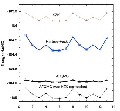
Figure 1: Comparison of the DFT, Hartree-Fock and AFQMC energy as a function of symmetrically inequivalent twist vector index for the four-atom NiO cell at the ambient volume. The twist vectors are chosen from a $\Gamma$-centered $4\times 4\times 4$ Monkhorst-Pack Monkhorst and Pack (1976); Pack and Monkhorst (1977) grid. The DFT simulations were performed using the KZK functional Giannozzi et al. (2009, 2017); Ma, Zhang, and Krakauer (2011) in a plane wave basis set while the Hartree-Fock and AFQMC simulations used the TZV2P basis. The KZK data have been shifted by -125.2 Ha/NiO for clarity.

In Fig. 2 we investigate the convergence of the AFQMC energy with respect to twist averaging as a function of volume. We see that a finer grid of twist vectors is required at higher densities (lower volumes). This can be understood as the system becomes more metallic and thus shell effects become more important.

In Fig. 3 we compare the raw and size-corrected AFQMC and KZK cold curves. We see that the KZK corrections generally shift the minimum of the AFQMC cold curve towards the experimental volume. However, the KZK corrections for this small supercell are still quite large. Larger simulations are required before the accuracy of AFQMC relative to experiment can be safely determined. Also plotted is the subplot of Fig. 3 is the correlation energy for the finite supercell.

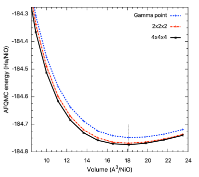
Figure 2: Comparison of the AFQMC cold curve for AFM-NiO obtained using different densities of twist vectors in the TZV2P basis. Curves are guides to the eyes. The dotted vertical line denotes the experimental value for the equilibrium volume. Bartel and Morosin (1971)

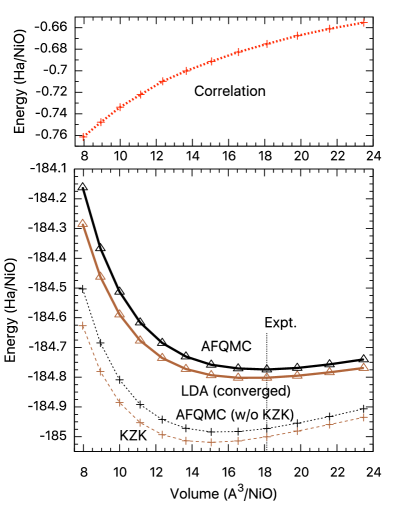
Figure 3: Comparison of cold curves calculated within DFT [using the KZK and local density approximation (LDA) functionals] and AFQMC for the 4-atom cell of NiO in the AFM-II state. The AFQMC simulations were performed using the TZV2P basis(Hutter et al., 2014). The KZK and AFQMC energies have been twist-averaged using a $\Gamma$-centered 4$\times$4$\times$4 $k$ Monkhorst-Pack grid. The converged LDA+U energies were calculated using a $\Gamma$-centered 8$\times$8$\times$8 Monkhorst-Pack grid. The dotted vertical line denotes the experimental value for the equilibrium volume. Bartel and Morosin (1971) For clarity, LDA and KZK data have been shifted by -126.3 Ha/NiO. The curves joining the points are meant as guides to the eye.

III.3 Basis Set Convergence

We next investigate the dependence of the AFQMC energy on basis set and the corresponding convergence rate of structural properties. Fig. 4 shows a comparison of the NiO cold curve, as calculated by AFQMC, for the various basis sets considered in this work; KZK size corrections have been applied and twist averaging was employed using a 4x4x4 twist grid. As expected, there is a systematic reduction in total energy as the basis set increases in size. From the figure it is clear that larger basis sets increase the equilibrium volume of the material, bringing results in closer agreement to experimental measurements. The change in equilibrium volume is large when moving from the DZVP to the TZVP basis, with results of 17.49 and 17.92 ų/NiO respectively. The change from TZVP to TZV2P is much smaller, TZV2P also having a volume of 17.92 ų/NiO. While the latter basis set is fairly close to convergence with respect to the complete basis set (CBS) limit, it is possible to obtain a reasonably accurate estimate of the bulk properties at the CBS limit by employing a standard basis set extrapolation scheme, very common in the quantum chemistry community when Gaussian basis sets are employed. In particular, we use the following formula to extrapolate the correlation energy contribution of the energy,

$$E_{c}(l_{\text{max}})=E_{c}^{\text{CBS}}+Al_{\text{max}}^{-3},$$ (37)

where $l_{\text{max}}$ denotes the highest angular momentum included in the basis set. The AFQMC energies obtained from the extrapolated values of the correlation energy, $E_{c}^{\text{CBS}}$, are shown in Fig. 4 with a solid red curve. Several things must be mentioned at this point regarding the extrapolated energies. First, the TZV2P basis lacks a basis function with angular momentum $l=4$, which is typically included in a triple-zeta quality basis set in calculations of finite molecular systems. This would somewhat affect the accuracy of the resulting energy extrapolation. In addition, typical extrapolation schemes in molecular calculations are based on three or more basis sets, in order to obtain highly accurate extrapolations to the CBS limit. Unfortunately, the lack of available basis sets beyond TZV2P prevents us from obtaining more accurate extrapolations at this time. Nonetheless, given the small magnitude of the correction and the fact that we are mainly interested in the volume dependence only (not in the total magnitude), we believe that the current extrapolation serves as a reliable estimate of the converged cold curve obtained from AFQMC for the current 4-atom cell studied in this work.

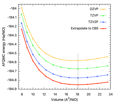
Figure 4: Comparison of AFQMC cold curve for AFM-NiO obtained using different basis sets. Results have been twist-averaged over a $\Gamma$-centered 4$\times$4$\times$4 $k$ grid and size-corrected with the KZK method. Curves are guides to the eyes. The dotted vertical line denotes the experimental value for the equilibrium volume. Bartel and Morosin (1971)

III.4 Comparison to other methods

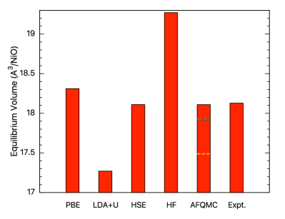
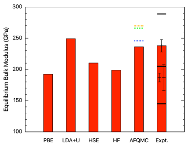
Figure 5: Comparison of the equilibrium volume and bulk modulus by fitting the cold curve from various methods to Murnaghan equation of state Murnaghan (1944). The scattered bars and data points in experimental bulk modulus denote different measurements Dudarev et al. (1998); Hua ; Huang (1995). AFQMC values shown with the red rectangles are the CBS limits obtained by extrapolating the DZVP and TZVP values using Eq. 37. The yellow dash-dotted, green dashed, and blue dotted bars denote corresponding AFQMC values using the DZVP, TZVP, and TZV2P basis, respectively.

Table 1: AFQMC values (CBS limits obtained by extrapolating the DZVP and TZVP values using Eq. 37) for the equilibrium volume $V_{0}$ and bulk modulus $B_{0}$ of NiO in rock-salt structure and anti-ferromagnetic state in comparison with experimental measurements and those from Hartree-Fock (HF) and DFT calculations, including PBE, localized density approximation plus Hubbard $U$ (LDA+$U$), PBE+$U$, and Heyd-Scuseria-Ernzerhof (HSE06) hybrid functional. Diffusion Monte Carlo (DMC) and selected DFT or HF simulations from literature Mitra et al. (2015) are also shown for comparison.

	$V_{0}$ (Å3/NiO)	$B_{0}$ (GPa)
AFQMC	18.11	236
DMC Mitra et al. (2015)	17.96$\pm$0.04	196$\pm$4
PBE	18.31	192
PBE Tran et al. (2006)	18.52	197
PBE Feng and Harrison (2004)	18.30	201
PBE Feng and Harrison (2004)	18.28	217
LDA Mitra et al. (2015)	16.73	232
LDA Tran et al. (2006)	16.85	257
PBE+U	18.74	214
LDA+U	17.27	249
LDA+U Mitra et al. (2015)	17.23	236
LDA+U Tran et al. (2006)	17.48	234
HSE06	18.11	210
HSE06 Mitra et al. (2015)	17.98	198
PBE0 Tran et al. (2006)	19.06	187
B3LYP Feng and Harrison (2004)	18.76	209
B3LYP Feng and Harrison (2004)	18.85	198
B3PW91 Tran et al. (2006)	18.65	203
Fock-0.35 Tran et al. (2006)	17.87	227
Fock-0.5 Tran et al. (2006)	18.26	218
HF	19.27	200
HF Dudarev et al. (1998)	19.33	–
Experiment	18.13Bartel and Morosin (1971)	166-208 Hua ,145,205,289 Dudarev et al. (1998)
	(0 K, $a_{0}$=4.171 Å)	187$\pm$7 Huang (1995),238$\pm$10 Huang (1995)

We obtained the NiO equilibrium volume ($V_{0}$) and bulk modulus ($B_{0}$) using a Murnaghan fit to the size-corrected AFQMC data(Murnaghan, 1944), and used Eq. 37 to extrapolate the resulting energies to the CBS limits using the corresponding DZVP and TZV2P calculations. The results are summarized in Table 1 and Fig. 5. We compare our results to UHF and spin-polarized DFT simulations for the same four-atom cell calculated using VASPKresse and Furthmüller (1996); Blöchl, Jepsen, and Andersen (1994); dft . To investigate the importance of the exchange correlation functional we tested the PBE Perdew, Burke, and Ernzerhof (1996) and Heyd-Scuseria-Ernzerhof (HSE06) Heyd, Scuseria, and Ernzerhof (2006) functionals as well as the LDA+$U$ Ceperley and Alder (1980); Perdew and Zunger (1981); Dudarev et al. (1998) and PBE+$U$ approaches. Our DFT and UHF results agree well with those from previous publications Dudarev et al. (1998); Tran et al. (2006); Feng and Harrison (2004).

We see from Fig. 5 that, in the CBS limit, AFQMC provides remarkably consistent results for both the equilibrium volume and bulk modulus, despite the possible remaining errors due to the use of KZK and basis set corrections. In contrast, the PBE, LDA$+U$ and HF results give significantly varied results. Overall, and as expected, DFT results exhibit a strong dependence on the choice of the exchange correlation functional. Of the functionals tested, the HSE06 functional performs best when compared with both the DMC results of Ref. Mitra et al., 2015 and the experimental equilibrium volume. The experimental data for the bulk modules is quite scattered so no real comparison can be made here.

IV Conclusion

In summary, we presented the application of the phaseless AFQMC method to a real, strongly correlated solid using periodic Gaussian basis sets. We investigated the importance of size corrections on AFQMC energies and on structural properties. We found that existing techniques to correct finite size errors in QMC work well even in strongly correlated materials and can be used in future studies on larger simulation cells. We present a detailed analysis of the influence of basis set on the structural properties of NiO in the AFM II state, obtaining results that are reasonably converged with respect to basis set size. We employ basis set extrapolation to obtain a correction for the energy missing when using our largest basis set, which we believe provides a meaningful estimate to the converged cold curve of NiO. We obtain excellent agreement with experimental measurements on the equilibrium volume. While these results are quite encouraging, this represent only the first step in a long journey whose final goal is the positioning of AFQMC as a method of choice in the study of strongly correlated materials. Ongoing work on NiO includes the study of larger basis sets and correlation-consistent effective-core potentials(ncs, ), the use of larger unit cells to eliminate the need for size correction schemes, and the study of other properties including spin gaps, excitation energies and the interplay of magnetism and bang-gap closure. Nonetheless, we believe that these preliminary calculations serve as a stepping stone in this direction.

Acknowledgement. We would like to thank Shiwei Zhang and Mario Motta for helpful discussions and Qiming Sun for assistance in running PySCF. S.Z. is in debt to Edgar Landinez for helpful discussions. This work was performed under the auspices of the U.S. Department of Energy (DOE) by LLNL under Contract No. DE-AC52-07NA27344. Funding support was from the U.S. DOE, Office of Science, Basic Energy Sciences, Materials Sciences and Engineering Division, as part of the Computational Materials Sciences Program and Center for Predictive Simulation of Functional Materials (CPSFM). Computer time was provided by the Argonne Leadership Computing and Livermore Computing Facilities.

References

- Sachdev (2008) S. Sachdev, Nature Physics 4, 173 (2008).
- Imada, Fujimori, and Tokura (1998) M. Imada, A. Fujimori, and Y. Tokura, Rev. Mod. Phys. 70, 1039 (1998).
- (3) P. Coleman, in Handbook of Magnetism and Advanced Magnetic Materials, Vol 1: Fundamentals and Theory, edited by H. Kronmuller and S. Parkin (John Wiley and Sons, 2007) Chap. 5, pp. 95–148.
- Si and Steglich (2010) Q. Si and F. Steglich, Science 329, 1161 (2010).
- Lee, Nagaosa, and Wen (2006) P. A. Lee, N. Nagaosa, and X.-G. Wen, Rev. Mod. Phys. 78, 17 (2006).
- Keimer et al. (2013) B. Keimer, S. A. Kivelson, M. R. Norman, S. Uchida, and J. Zaanen, Nature 518, 179 (2013).
- Hubbard (1963) J. Hubbard, Proc. Royal Soc. Lond, Ser. A 276, 238 (1963).
- Hohenberg and Kohn (1964) P. Hohenberg and W. Kohn, Phys. Rev. 136, B864 (1964).
- Kohn and Sham (1965) W. Kohn and L. J. Sham, Phys. Rev. 140, A1133 (1965).
- Heyd, Scuseria, and Ernzerhof (2006) J. Heyd, G. E. Scuseria, and M. Ernzerhof, The Journal of Chemical Physics 124, 219906 (2006).
- Perdew, Ernzerhof, and Burke (1996) J. P. Perdew, M. Ernzerhof, and K. Burke, The Journal of Chemical Physics 105, 9982 (1996).
- Adamo and Barone (1999) C. Adamo and V. Barone, The Journal of Chemical Physics 110, 6158 (1999).
- Lee, Yang, and Parr (1988) C. Lee, W. Yang, and R. G. Parr, Phys. Rev. B 37, 785 (1988).
- Becke (1993) A. D. Becke, J. Chem. Phys. 98, 5648 (1993).
- Dudarev et al. (1998) S. L. Dudarev, G. A. Botton, S. Y. Savrasov, C. J. Humphreys, and A. P. Sutton, Phys. Rev. B 57, 1505 (1998).
- Onida, Reining, and Rubio (2002) G. Onida, L. Reining, and A. Rubio, Rev. Mod. Phys. 74, 601 (2002).
- Georges et al. (1996) A. Georges, G. Kotliar, W. Krauth, and M. J. Rozenberg, Rev. Mod. Phys. 68, 13 (1996).
- Kotliar et al. (2006) G. Kotliar, S. Y. Savrasov, K. Haule, V. S. Oudovenko, O. Parcollet, and C. A. Marianetti, Rev. Mod. Phys. 78, 865 (2006).
- Anisimov et al. (1997) V. I. Anisimov, A. I. Poteryaev, M. A. Korotin, A. O. Anokhin, and G. Kotliar, Journal of Physics: Condensed Matter 9, 7359 (1997).
- Ren et al. (2006) X. Ren, I. Leonov, G. Keller, M. Kollar, I. Nekrasov, and D. Vollhardt, Phys. Rev. B 74, 195114 (2006).
- Leonov et al. (2016) I. Leonov, L. Pourovskii, A. Georges, and I. A. Abrikosov, Phys. Rev. B 94, 155135 (2016).
- Carter (2008) E. A. Carter, Science 321, 800 (2008).
- Zhang, Carlson, and Gubernatis (1997) S. Zhang, J. Carlson, and J. E. Gubernatis, Phys. Rev. B 55, 7464 (1997).
- Zhang and Krakauer (2003) S. Zhang and H. Krakauer, Phys. Rev. Lett. 90, 136401 (2003).
- Motta and Zhang (2017a) M. Motta and S. Zhang, J. Chem. Theory Comput. 13, 5367 (2017a).
- Ma, Zhang, and Krakauer (2013) F. Ma, S. Zhang, and H. Krakauer, New J. Phys. 15, 093017 (2013).
- Motta et al. (2014) M. Motta, D. E. Galli, S. Moroni, and E. Vitali, J. Chem. Phys. 140, 024107 (2014).
- Vitali et al. (2016) E. Vitali, H. Shi, M. Qin, and S. Zhang, Phys. Rev. B 94, 085140 (2016).
- Motta and Zhang (2018) M. Motta and S. Zhang, J. Chem. Phys. 148, 181101 (2018).
- Suewattana et al. (2007) M. Suewattana, W. Purwanto, S. Zhang, H. Krakauer, and E. J. Walter, Phys. Rev. B 75, 245123 (2007).
- Ma, Zhang, and Krakauer (2017) F. Ma, S. Zhang, and H. Krakauer, Phys. Rev. B 95, 165103 (2017).
- Purwanto, Zhang, and Krakauer (2013) W. Purwanto, S. Zhang, and H. Krakauer, J. Chem. Theory Comput. 9, 4825 (2013), pMID: 26583401, https://doi.org/10.1021/ct4006486 .
- Purwanto, Zhang, and Krakauer (2009) W. Purwanto, S. Zhang, and H. Krakauer, J. Chem. Phys. 130, 094107 (2009).
- Borda, Gomez, and Morales (2018) E. J. L. Borda, J. A. Gomez, and M. A. Morales, arXiv preprint arXiv:1801.10307 (2018).
- Qin, Shi, and Zhang (2016a) M. Qin, H. Shi, and S. Zhang, Phys. Rev. B 94, 085103 (2016a).
- Chang and Morales (2017) C.-C. Chang and M. A. Morales, arXiv preprint arXiv:1711.02154 (2017).
- Qin, Shi, and Zhang (2016b) M. Qin, H. Shi, and S. Zhang, Phys. Rev. B 94, 235119 (2016b).
- Zheng et al. (2017) B.-X. Zheng, C.-M. Chung, P. Corboz, G. Ehlers, M.-P. Qin, R. M. Noack, H. Shi, S. R. White, S. Zhang, and G. K.-L. Chan, Science 358, 1155 (2017).
- LeBlanc et al. (2015) J. P. F. LeBlanc, A. E. Antipov, F. Becca, I. W. Bulik, G. K.-L. Chan, C.-M. Chung, Y. Deng, M. Ferrero, T. M. Henderson, C. A. Jiménez-Hoyos, E. Kozik, X.-W. Liu, A. J. Millis, N. V. Prokof’ev, M. Qin, G. E. Scuseria, H. Shi, B. V. Svistunov, L. F. Tocchio, I. S. Tupitsyn, S. R. White, S. Zhang, B.-X. Zheng, Z. Zhu, and E. Gull (Simons Collaboration on the Many-Electron Problem), Phys. Rev. X 5, 041041 (2015).
- Motta et al. (2017) M. Motta, D. M. Ceperley, G. K.-L. Chan, J. A. Gomez, E. Gull, S. Guo, C. A. Jiménez-Hoyos, T. N. Lan, J. Li, F. Ma, A. J. Millis, N. V. Prokof’ev, U. Ray, G. E. Scuseria, S. Sorella, E. M. Stoudenmire, Q. Sun, I. S. Tupitsyn, S. R. White, D. Zgid, and S. Zhang (Simons Collaboration on the Many-Electron Problem), Phys. Rev. X 7, 031059 (2017).
- Ma et al. (2015) F. Ma, W. Purwanto, S. Zhang, and H. Krakauer, Phys. Rev. Lett. 114, 226401 (2015).
- Foulkes et al. (2001) W. M. C. Foulkes, L. Mitas, R. J. Needs, and G. Rajagopal, Rev. Mod. Phys. 73, 33 (2001).
- Nazarov et al. (2016) R. Nazarov, L. Shulenburger, M. Morales, and R. Q. Hood, Phys. Rev. B 93, 094111 (2016).
- Schiller, Wagner, and Ertekin (2015) J. A. Schiller, L. K. Wagner, and E. Ertekin, Phys. Rev. B 92, 235209 (2015).
- Mitra et al. (2015) C. Mitra, J. T. Krogel, J. A. Santana, and F. A. Reboredo, The Journal of Chemical Physics 143, 164710 (2015).
- Wagner and Ceperley (2016) L. K. Wagner and D. M. Ceperley, Rep. Prog. Phys. 79, 094501 (2016).
- Shin et al. (2017) H. Shin, Y. Luo, P. Ganesh, J. Balachandran, J. T. Krogel, P. R. C. Kent, A. Benali, and O. Heinonen, Phys. Rev. Materials 1, 073603 (2017).
- Motta and Zhang (2017b) M. Motta and S. Zhang, arXiv preprint arXiv:1711.02242 (2017b).
- Booth, Thom, and Alavi (2009) G. H. Booth, A. J. W. Thom, and A. Alavi, The Journal of Chemical Physics 131, 054106 (2009).
- Thouless (1960) D. J. Thouless, Nuc. Phys. 21, 225 (1960).
- Hubbard (1959) J. Hubbard, Phys. Rev. Lett. 3, 77 (1959).
- Al-Saidi, Krakauer, and Zhang (2006a) W. A. Al-Saidi, H. Krakauer, and S. Zhang, Phys. Rev. B 73, 075103 (2006a).
- Al-Saidi, Zhang, and Krakauer (2006) W. A. Al-Saidi, S. Zhang, and H. Krakauer, J. Chem. Phys. 124, 224101 (2006).
- Al-Saidi, Krakauer, and Zhang (2006b) W. A. Al-Saidi, H. Krakauer, and S. Zhang, J. Chem. Phys. 125, 154110 (2006b).
- Al-Saidi, Krakauer, and Zhang (2007) W. A. Al-Saidi, H. Krakauer, and S. Zhang, J. Chem. Phys. 126, 194105 (2007).
- Purwanto, Krakauer, and Zhang (2009) W. Purwanto, H. Krakauer, and S. Zhang, Phys. Rev. B 80, 214116 (2009).
- Gillan et al. (2008) M. J. Gillan, D. Alfè, S. d. Gironcoli, and F. R. Manby, J. Comp. Chem. 29, 2098 (2008).
- Nolan et al. (2009) S. J. Nolan, M. J. Gillan, D. Alfè, N. L. Allan, and F. R. Manby, Phys. Rev. B 80 (2009).
- Booth et al. (2013) G. H. Booth, A. Grüneis, G. Kresse, and A. Alavi, Nature 493, 365 (2013).
- McClain et al. (2017) J. McClain, Q. Sun, G. K.-L. Chan, and T. C. Berkelbach, J. Chem. Theory Comput. 13, 1209 (2017).
- Sun et al. (2017) Q. Sun, T. C. Berkelbach, J. D. McClain, and G. K.-L. Chan, J. Chem. Phys. 147, 164119 (2017).
- Sun et al. (2018) Q. Sun, T. C. Berkelbach, N. S. Blunt, G. H. Booth, S. Guo, Z. Li, J. Liu, J. D. McClain, E. R. Sayfutyarova, S. Sharma, S. Wouters, and G. K. Chan, Wiley Interdisciplinary Reviews: Computational Molecular Science 8, e1340 (2018).
- F. and Jan (1977) B. N. H. F. and L. Jan, Int. J. Quantum Chem. 12, 683 (1977).
- Koch, de Merás, and Pedersen (2003) H. Koch, A. S. de Merás, and T. B. Pedersen, J. Chem. Phys. 118, 9481 (2003).
- Francesco et al. (2009) A. Francesco, D. V. Luca, F. Nicolas, G. Giovanni, M. Per‐åke, N. Pavel, P. T. Bondo, P. Michal, R. Markus, R. B. O., S. Luis, U. Miroslav, V. Valera, and L. Roland, J. Comput. Chem. 31, 224 (2009).
- Purwanto et al. (2011) W. Purwanto, H. Krakauer, Y. Virgus, and S. Zhang, J. Chem. Phys. 135, 164105 (2011).
- Purwanto and Zhang (2004) W. Purwanto and S. Zhang, Phys. Rev. E 70, 056702 (2004).
- Tran et al. (2006) F. Tran, P. Blaha, K. Schwarz, and P. Novák, Phys. Rev. B 74, 155108 (2006).
- Feng and Harrison (2004) X.-B. Feng and N. M. Harrison, Phys. Rev. B 69, 035114 (2004).
- Cohen, Mazin, and Isaak (1997) R. E. Cohen, I. I. Mazin, and D. G. Isaak, Science 275, 654 (1997).
- Kobayashi et al. (2008) S. Kobayashi, Y. Nohara, S. Yamamoto, and T. Fujiwara, Phys. Rev. B 78, 155112 (2008).
- Eder (2015) R. Eder, Phys. Rev. B 91, 245146 (2015).
- Shull, Strauser, and Wollan (1951) C. G. Shull, W. A. Strauser, and E. O. Wollan, Phys. Rev. 83, 333 (1951).
- Roth (1958a) W. L. Roth, Phys. Rev. 110, 1333 (1958a).
- Roth (1958b) W. L. Roth, Phys. Rev. 111, 772 (1958b).
- Roth and Slack (1960) W. L. Roth and G. A. Slack, Journal of Applied Physics 31, S352 (1960).
- Eto et al. (2000) T. Eto, S. Endo, M. Imai, Y. Katayama, and T. Kikegawa, Phys. Rev. B 61, 14984 (2000).
- Noguchi et al. (1999) Y. Noguchi, M. Uchino, H. Hikosaka, T. Atou, K. Kusaba, K. Fukuoka, T. Mashimo, and Y. Syono, Journal of Physics and Chemistry of Solids 60, 509 (1999).
- Shen et al. (1991) Z.-X. Shen, R. S. List, D. S. Dessau, B. O. Wells, O. Jepsen, A. J. Arko, R. Barttlet, C. K. Shih, F. Parmigiani, J. C. Huang, and P. A. P. Lindberg, Phys. Rev. B 44, 3604 (1991).
- Schuler et al. (2005) T. M. Schuler, D. L. Ederer, S. Itza-Ortiz, G. T. Woods, T. A. Callcott, and J. C. Woicik, Phys. Rev. B 71, 115113 (2005).
- Olalde-Velasco et al. (2011) P. Olalde-Velasco, J. Jiménez-Mier, J. D. Denlinger, Z. Hussain, and W. L. Yang, Phys. Rev. B 83, 241102 (2011).
- Goedecker, Teter, and Hutter (1996) S. Goedecker, M. Teter, and J. Hutter, Phys. Rev. B 54, 1703 (1996).
- Perdew, Burke, and Ernzerhof (1996) J. P. Perdew, K. Burke, and M. Ernzerhof, Phys. Rev. Lett. 77, 3865 (1996).
- VandeVondele and Hutter (2007) J. VandeVondele and J. Hutter, J. Chem. Phys. 127, 114105 (2007).
- Hutter et al. (2014) J. Hutter, M. Iannuzzi, F. Schiffmann, and J. VandeVondele, Wiley Interdisciplinary Reviews: Computational Molecular Science 4, 15 (2014).
- Note (1) For Ni, we use are short-range basis sets, MOLOPT-SR-GTH, which are more appropriate for solid state calculations. For O, the short-range basis is available only for DZVP, therefore we use the regular basis set (non-SR ones) for TZVP and TZV2P calculations. Our -point calculations show that the difference in the cold curve when switching from DZVP-MOLOPT-SR-GTH to DZVP-MOLOPT-GTH basis for O is negligible and leads to changes in and by only 0.4% and 3 GPa, respectively.
- Kim et al. (2018) J. Kim, A. T. Baczewski, T. D. Beaudet, A. Benali, M. C. Bennett, M. A. Berrill, N. S. Blunt, E. J. L. Borda, M. Casula, D. M. Ceperley, S. Chiesa, B. K. Clark, R. C. C. III, K. T. Delaney, M. Dewing, K. P. Esler, H. Hao, O. Heinonen, P. R. C. Kent, J. T. Krogel, I. Kylänpää, Y. W. Li, M. G. Lopez, Y. Luo, F. D. Malone, R. M. Martin, A. Mathuriya, J. McMinis, C. A. Melton, L. Mitas, M. A. Morales, E. Neuscamman, W. D. Parker, S. D. P. Flores, N. A. Romero, B. M. Rubenstein, J. A. R. Shea, H. Shin, L. Shulenburger, A. F. Tillack, J. P. Townsend, N. M. Tubman, B. V. D. Goetz, J. E. Vincent, D. C. Yang, Y. Yang, S. Zhang, and L. Zhao, Journal of Physics: Condensed Matter 30, 195901 (2018).
- Drummond et al. (2008) N. D. Drummond, R. J. Needs, A. Sorouri, and W. M. C. Foulkes, Phys. Rev. B 78, 125106 (2008).
- Holzmann et al. (2016) M. Holzmann, R. C. Clay, M. A. Morales, N. M. Tubman, D. M. Ceperley, and C. Pierleoni, Phys. Rev. B 94, 035126 (2016).
- Lin, Zong, and Ceperley (2001) C. Lin, F. H. Zong, and D. M. Ceperley, Phys. Rev. E 64, 016702 (2001).
- Fraser et al. (1996) L. M. Fraser, W. M. C. Foulkes, G. Rajagopal, R. J. Needs, S. D. Kenny, and A. J. Williamson, Phys. Rev. B 53, 1814 (1996).
- Chiesa et al. (2006) S. Chiesa, D. M. Ceperley, R. M. Martin, and M. Holzmann, Phys. Rev. Lett. 97, 076404 (2006).
- Kwee, Zhang, and Krakauer (2008) H. Kwee, S. Zhang, and H. Krakauer, Phys. Rev. Lett. 100, 126404 (2008).
- Ma, Zhang, and Krakauer (2011) F. Ma, S. Zhang, and H. Krakauer, Phys. Rev. B 84, 155130 (2011).
- Spink, Needs, and Drummond (2013) G. G. Spink, R. J. Needs, and N. D. Drummond, Phys. Rev. B 88, 085121 (2013).
- Azadi and Foulkes (2015) S. Azadi and W. M. C. Foulkes, J. Chem. Phys. 143, 102807 (2015).
- Monkhorst and Pack (1976) H. J. Monkhorst and J. D. Pack, Phys. Rev. B 13, 5188 (1976).
- Pack and Monkhorst (1977) J. D. Pack and H. J. Monkhorst, Phys. Rev. B 16, 1748 (1977).
- Giannozzi et al. (2009) P. Giannozzi, S. Baroni, N. Bonini, M. Calandra, R. Car, C. Cavazzoni, D. Ceresoli, G. L. Chiarotti, M. Cococcioni, I. Dabo, A. D. Corso, S. de Gironcoli, S. Fabris, G. Fratesi, R. Gebauer, U. Gerstmann, C. Gougoussis, A. Kokalj, M. Lazzeri, L. Martin-Samos, N. Marzari, F. Mauri, R. Mazzarello, S. Paolini, A. Pasquarello, L. Paulatto, C. Sbraccia, S. Scandolo, G. Sclauzero, A. P. Seitsonen, A. Smogunov, P. Umari, and R. M. Wentzcovitch, Journal of Physics: Condensed Matter 21, 395502 (2009).
- Giannozzi et al. (2017) P. Giannozzi, O. Andreussi, T. Brumme, O. Bunau, M. Buongiorno Nardelli, M. Calandra, R. Car, C. Cavazzoni, D. Ceresoli, M. Cococcioni, N. Colonna, I. Carnimeo, A. Dal Corso, S. de Gironcoli, P. Delugas, R. A. DiStasio, Jr., A. Ferretti, A. Floris, G. Fratesi, G. Fugallo, R. Gebauer, U. Gerstmann, F. Giustino, T. Gorni, J. Jia, M. Kawamura, H.-Y. Ko, A. Kokalj, E. Küçükbenli, M. Lazzeri, M. Marsili, N. Marzari, F. Mauri, N. L. Nguyen, H.-V. Nguyen, A. Otero-de-la-Roza, L. Paulatto, S. Poncé, D. Rocca, R. Sabatini, B. Santra, M. Schlipf, A. P. Seitsonen, A. Smogunov, I. Timrov, T. Thonhauser, P. Umari, N. Vast, X. Wu, and S. Baroni, Journal of Physics Condensed Matter 29, 465901 (2017).
- Bartel and Morosin (1971) L. C. Bartel and B. Morosin, Phys. Rev. B 3, 1039 (1971).
- Murnaghan (1944) F. D. Murnaghan, Proceedings of the National Academy of Sciences 30, 244 (1944).
- (103) E. Huang, K. Jy, S.-C. Yu, J. Geophys. Soc. China 37, 7 (1994).
- Huang (1995) E. Huang, High Pressure Research 13, 307 (1995).
- Kresse and Furthmüller (1996) G. Kresse and J. Furthmüller, Phys. Rev. B 54, 11169 (1996).
- Blöchl, Jepsen, and Andersen (1994) P. E. Blöchl, O. Jepsen, and O. K. Andersen, Phys. Rev. B 49, 16223 (1994).
- (107) In our VASP simulations, we use a 4-atom unit cell, -centered 888 Monkhorst-Pack mesh, a plane-wave basis with cutoff of 1200 eV, and a SCF convergence criteria of eV/cell. The PBE, HSE06, and HF simulations use the PAW pseudopotentials labeled with GW, and core radii equalling 2.3 and 1.6 Bohr for Ni and O, respectively. In the LDA+ calculations, we use PAW pseudopotentials with core radii equalling 2.0 and 1.1 Bohr for Ni and O, respectively. In the PBE+ calculations, we use hard PAW pseudopotentials with core radii equalling 2.0 and 1.1 Bohr for Ni and O, respectively. Except for the PBE+ case where take as valence electrons for Ni, we have taken and as valence electrons for Ni and O, respectively. In LDA+ calculations, we choose the method by Dudarev et al. Dudarev et al. (1998) with =5 eV for Ni.
- Ceperley and Alder (1980) D. M. Ceperley and B. J. Alder, Phys. Rev. Lett. 45, 566 (1980).
- Perdew and Zunger (1981) J. P. Perdew and A. Zunger, Phys. Rev. B 23, 5048 (1981).
- (110) Https://pseudopotentiallibrary.org.