Stellar models with calibrated convection and temperature stratification from 3D hydrodynamics simulations

Abstract

Stellar evolution codes play a major role in present-day astrophysics, yet they share common simplifications related to the outer layers of stars. We seek to improve on this by the use of results from realistic and highly detailed 3D hydrodynamics simulations of stellar convection. We implement a temperature stratification extracted directly from the 3D simulations into two stellar evolution codes to replace the simplified atmosphere normally used. Our implementation also contains a non-constant mixing-length parameter, which varies as a function of the stellar surface gravity and temperature – also derived from the 3D simulations. We give a detailed account of our fully consistent implementation and compare to earlier works, and also provide a freely available mesa-module. The evolution of low-mass stars with different masses is investigated, and we present for the first time an asteroseismic analysis of a standard solar model utilising calibrated convection and temperature stratification from 3D simulations. We show that the inclusion of 3D results have an almost insignificant impact on the evolution and structure of stellar models – the largest effect are changes in effective temperature of order $30\,\text{K}$ seen in the pre-main sequence and in the red-giant branch. However, this work provides the first step for producing self-consistent evolutionary calculations using fully incorporated 3D atmospheres from on-the-fly interpolation in grids of simulations.

1 Introduction

Understanding stellar structure and evolution is one of the key ingredients in astrophysics. One of the primary tools for doing so is comparing numerical calculations of stellar structure with observations and analysing changes in time using a stellar evolution code. These are one-dimensional (1D) numerical models, which have been tested and developed through the years; as a result they are very efficient and highly optimised. However, in several aspects they are also simplified and can be improved.

The first problem we address in this paper is related to the outer boundary conditions of the models, which are required to solve the stellar equations. Traditionally they are established by integration of a simplified temperature stratification as a function of optical depth – a so-called $T(\tau)$ relation– which combined with hydrostatic equilibrium provides the pressure for the outermost point in the model. The most commonly used is the analytical grey Eddington atmosphere (e.g. Kippenhahn et al., 2012); other popular choices are semi-empirical relations derived from the Sun (Krishna Swamy, 1966; Vernazza et al., 1981). The $T(\tau)$ relation (also commonly known as the atmosphere) employed in the model has a non-negligible impact on the structure and evolution (see, e.g. Salaris et al., 2002; Tanner et al., 2014).

Secondly we address one of the most fundamental problems in stellar physics: the treatment of stellar convection. The most adopted method for parametrising this process in stellar evolution calculations is the formalism from Böhm-Vitense (1958) known as the mixing-length theory (MLT). The basic idea in MLT is to model convection as rising and falling elements, which move in a background medium. The background is the mean stratification where pressure equilibrium is assumed as well as symmetry between the up- and downflows. A convective element moves a certain distance $\Lambda$ before dissolving/mixing instantaneously into the ambient medium. This distance (called the mixing length) is assumed proportional to the local pressure scale height $H_{\textup{p}}$ as $\Lambda=\alpha_{\textup{\tiny MLT}}H_{\textup{p}}$, where $\alpha_{\textup{\tiny MLT}}$ is the central free parameter of the theory: the mixing-length parameter.

Usually the value of $\alpha_{\textup{\tiny MLT}}$ is constrained by the Sun. However, in several recent studies on the detailed modelling of red-giant stars, $\alpha_{\textup{\tiny MLT}}$ has been highlighted as a focus point. For instance Li et al. (2018) reported the need of modifying $\alpha_{\textup{\tiny MLT}}$ in the RGB by using eclipsing binaries from Kepler as calibrators. Tayar et al. (2017) found similar problems based on several thousand red giants – although this claim has been disputed in the very recent work by Salaris et al. (2018). Hjørringgaard et al. (2017) have reported on discrepancies between constraints from different independent methods when determining the parameters of the very well-studied red giant HD 185351. Moreover, the problem of an unconstrained $\alpha_{\textup{\tiny MLT}}$ is not unique to red giants: White et al. (2017) showed that their parameter determinations using mesa changed significantly when $\alpha_{\textup{\tiny MLT}}$ was free to vary compared to a fixed solar value.

Another very different approach to superadiabatic convection in the outer layers of stars is to make a full three-dimensional (3D) simulation using radiation-coupled hydrodynamics (RHD). These simulations cover both the radiative outer atmosphere as well as the superadiabatic convective sub-photospheric layers, reaching the quasi-adiabatic deeper convective layers. No parametric theory is needed to generate the convection; only fundamental physics. These simulations are inherently more realistic, and have become very popular in recent years. The 3D simulations have produced impressive results – e.g. being able to reproduce the observed solar granulation from first principles (Stein & Nordlund, 1998) – and have altered our understanding of stellar convection (e.g. Stein & Nordlund, 1989; Nordlund et al., 2009). A major drawback of this kind of simulations is that they are computationally very expensive. Moreover, the simulations are designed to study the stellar granulation, which operates on very short timescales compared to nuclear processes in the star. Thus, these simulations cannot be directly utilised to calculate stellar evolution models, as they are not able to follow the timescales required.

In this work, we seek to remedy some of the issues in stellar evolution models by the use of results from the realistic and highly detailed 3D RHD simulations of stellar convection. The ultimate goal is to employ full structures from the 3D simulations on-the-fly in stellar evolutionary calculations, thus producing the next generation of stellar models. This paper – which continues the work of Mosumgaard et al. (2017) – is a major step in the pursuit of this.

The paper is organised as follows. In the next section, a description of the 3D simulations and the data used is given. We present our implementation in some detail in Section 3 and the impact of using it in evolutionary and asteroseismic calculations in Section 4. In Section 5 we present a discussion, where we also compare our implementation with the previous work by Salaris & Cassisi (2015) – also elaborated in Appendix B – and finally a conclusion in Section 6. In Appendix A we review the technical details of our mesa-module, which we make freely available.

2 3D simulations of stellar atmospheres

We have used data from the grid of 37 atmospheric 3D simulations of stellar convection by Trampedach et al. (2013, 2014a, 2014b). All of the simulations are computed with solar metallicity and the coverage in a Kiel diagram (effective temperature $T_{\textup{eff}}$ and surface gravity $\log g$) is shown in Fig. 1. It should be noted that the simulations were calculated using a non-standard solar composition based on Anders & Grevesse (1989, AG89); the exact composition – which is actually very close to Grevesse & Noels (1993, GN93) – is given in Trampedach et al. (2013, Table 1).

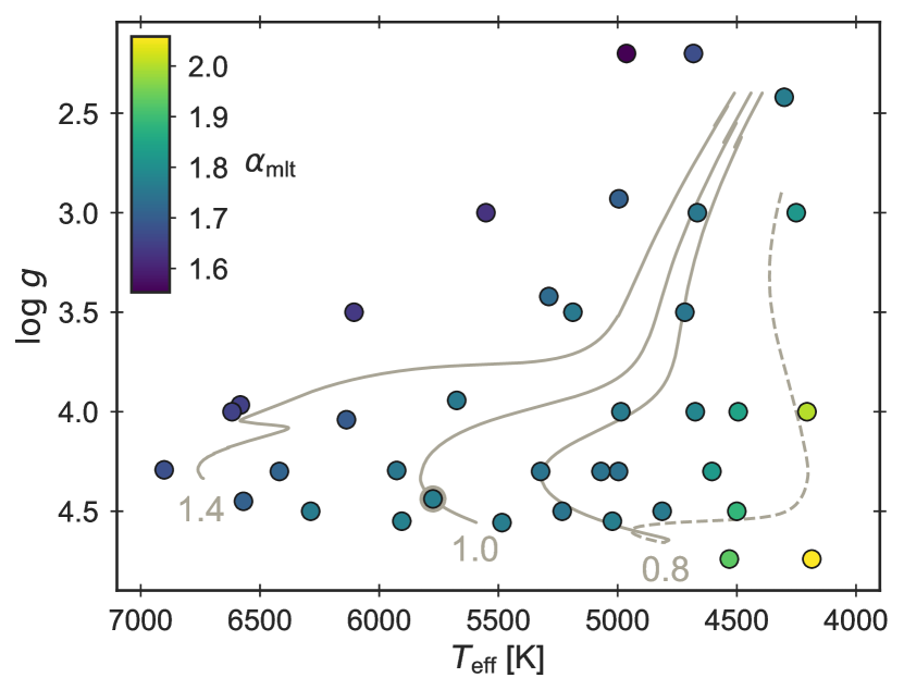
Figure 1: A Kiel diagram, in terms of effective temperature $T_{\textup{eff}}$ and logarithm of surface gravity $g$, showing the grid of 3D simulations at solar metallicity coloured to show the corresponding value of the calibrated mixing-length parameter $\alpha_{\textup{\tiny MLT}}$ from Trampedach et al. (2014b). Evolutionary tracks from garstec for stars of different masses (in units of the mass of the Sun) are shown for reference – the pre-main sequence for one of the tracks are shown with dashes.

2.1 Patched models

The most common synergy between 3D convection simulations and typical stellar evolution models are the so-called patched models. The principle in producing a patched model is to peel off the surface layers of a stellar structure model and replace it with data from a 3D simulation averaged over time and the horizontal directions. Great care must be taken in ensuring a correct and compatible patching between the two different parts – e.g. by using similar microphysics and boundary conditions (Trampedach et al., 2014a). Several authors have utilised this technique and it has primarily been applied in helio- and asteroseismology to investigate the so-called asteroseismic surface effect (Brown, 1984; Christensen-Dalsgaard et al., 1988), as the procedure naturally alters the outer regions in the models.

The technique was originally applied to the Sun by Rosenthal et al. (1999), and later by Piau et al. (2014) and Magic & Weiss (2016). It has also been used in analyses across different stellar parameters by e.g. Sonoi et al. (2015), Ball et al. (2016), and Trampedach et al. (2017). The advantage of this method is that the poorly modelled surface layers of the stellar model are fully replaced by the sophisticated 3D structure, which significantly diminishes the surface effect. However, the method comes with two primary disadvantages.

A first clear issue is that the simulations only sample discrete points in the HR diagram. Thus, in order to patch, the interior model must correspond to a specific 3D simulation, making it impractical when modelling “real” stars. This part of the problem has been treated by Jørgensen et al. (2017), who developed a technique for interpolating between the 3D simulations in a grid. The work utilized the interpolation scheme for producing the patched models with arbitrary physical parameters, and applied the method to several stars observed by the Kepler space mission (Borucki et al., 2010). In fact Jørgensen et al. (2017) calculated their pre-patching evolution using the garstec-implementation described in this paper, before patching with the corresponding 3D simulations, to ensure the highest level of consistency.

Secondly, it is not possible to do time evolution with the patched models. It is a purely static approach: The 1D model is evolved using a regular boundary condition until a certain point, where it is then patched to a corresponding 3D simulation. Stellar evolution is the main focus of the dynamic implementation we present in the following.

2.2 Condensed simulations

As a first step to overcoming some of the problems, Trampedach et al. (2014a, b) developed a method for extracting information from the 3D simulations targeted at the two issues mentioned above.

Firstly, they have used 1D envelope models to calibrate the mixing-length parameter, $\alpha_{\textup{\tiny MLT}}$, for each simulation. The basic principle behind the calibration is similar to the patching procedure described before, but using envelope models instead of full structure models – and of course varying $\alpha_{\textup{\tiny MLT}}$ as a part of the process. The authors went to great length to ensure compatible (micro)physics between their 1D and 3D models. The exact procedure is described by Trampedach et al. (2014b) and the resulting values are visualised in Fig. 1. Stellar evolution tracks of different masses are also shown in the figure to display the coverage of the grid. A similar work was done using 2D simulations by Ludwig et al. (1999), who found similar trends with stellar parameters.

Secondly, the authors devised a way of distilling the averaged temperature stratification from the full 3D simulations. They have taken great care in the treatment of convective effects and enforcing radiative equilibrium; a detailed description is given by Trampedach et al. (2014a). The output is given in the form of a generalised Hopf function $q(\tau)$ given as

$$\frac{4}{3}\left(\frac{T}{T_{\textup{eff}}}\right)^{4}=q(\tau)+\tau\;,$$ (1)

where $\tau$ is a Rosseland mean optical depth (Trampedach et al., 2014a, eq. 9). It is important to note that these extracted $T(\tau)$ relations were also used in Trampedach et al. (2014b) to perform the $\alpha_{\textup{\tiny MLT}}$-calibration mentioned above in order to ensure maximum consistency.

The results provided by Trampedach et al. (2014a, b) – i.e $q(\tau)$ and calibrated $\alpha_{\textup{\tiny MLT}}$ for all simulations – are stored as a function of $T_{\textup{eff}}$ and $\log g$. The main advantage of the described approach is that the extracted quantities behave smoothly with varying $T_{\textup{eff}}$ and $\log g$, making it feasible to directly interpolate between the simulations. Thus, it is possible to include the 3D effects during the evolution of stars within the full range of the grid of simulations.

3 Implementation

We have consistently implemented the use of information from 3D atmospheric simulations from Trampedach et al. (2014a, b) into the Garching Stellar Evolution Code (garstec, Weiss & Schlattl, 2008) and Modules for Experiments in Stellar Astrophysics (mesa, Paxton et al., 2011; Paxton et al., 2013, 2015). The basic principle of our implementation is that in each iteration of the stellar evolution code, the current $T_{\textup{eff}}$ and $\log g$ of the model are used to obtain corresponding information from the 3D simulations. More specifically we extract the $\alpha_{\textup{\tiny MLT}}$ and corresponding $q(\tau)$ – which can be transformed to a $T(\tau)$ relation (see below) – from a table as a function of $T_{\textup{eff}}$ and $\log g$. To interpolate in the irregular grid of simulations, we use the routine supplied by Trampedach et al. (2014a, b), which is based on linear interpolation between the nodes in a Thiessen triangulation (Cline & Renka, 1984).

3.1 Mixing-length parameter

The first change to the stellar structure model involves the mixing-length parameter, which is vital for the treatment of convection. Instead of a constant value we use the variable 3D-calibrated mixing-length parameter, $\alpha_{\textup{\tiny MLT}}(T_{\textup{eff}},\log g)$, throughout the model.

We are not taking the value directly as provided by the interpolation in the table, but introduce a scaling factor as recommended by Ludwig et al. (1999) and Trampedach et al. (2014b). The actual $\alpha_{\textup{\tiny MLT}}$ used in the code is given by

$$\alpha_{\textup{\tiny MLT}}(T_{\textup{eff}},\log g)=K_{\textup{\tiny MLT}}\cdot\alpha_{\textup{{\tiny MLT}, grid}}(T_{\textup{eff}},\log g)\;,$$ (2)

where $K_{\textup{\tiny MLT}}$ is the scaling factor and $\alpha_{\textup{{\tiny MLT}, grid}}$ is the value returned from the interpolation routine.

The scaling factor must be determined from a solar calibration with the 3D $T(\tau)$ relation (see below) and variable mixing-length parameter activated. This scaling ensures that the solar model is calibrated to the correct radius with the variable $\alpha_{\textup{\tiny MLT}}$.

3.2 $T(\tau)$ relation

The other aspect of our implementation is related to the use of a realistic $T(\tau)$ relation derived from the 3D simulations. As mentioned above, the interpolation routine supplies the current stratification (updated in each iteration) as a function of optical depth, $\tau$, in terms of the generalised Hopf function, $q(\tau)$.

The changes made in garstec and mesa are nearly identical. We provide a detailed account of the garstec implementation and at the end highlight how the modifications in the two codes differ. We will split the description in two (one for each part of a garstec structure model): atmosphere and interior.

3.2.1 Atmospheric part

The atmospheric part of the model is used to provide the outer boundary conditions for the equations of stellar structure and evolution. In the standard setting, the code uses an Eddington grey atmosphere, which is anchored to the interior model at an optical depth of $\tau=2/3$.

In our implementations, we have altered the atmospheric module to obtain the temperature stratification from the generalised Hopf function $q(\tau)$ extracted from the 3D simulations. The new temperature structure at a given optical depth can be obtained from eq. (1) as

$$T(\tau)=\left(\frac{3}{4}\right)^{1/4}\left[q(\tau)+\tau\right]^{1/4}T_{\textup{eff}}\;,$$ (3)

under the assumption of radiative equilibrium.

In garstec, the stratification is integrated inwards from $\tau_{\textup{surf}}=10^{-4}$ to obtain the pressure at the bottom of the atmosphere. This point is the fitting point or transition point to the interior model – commonly referred to as the photosphere – which is defined to have the temperature $T=T_{\textup{eff}}$. As opposed to the Eddington grey case, the 3D $T(\tau)$ relation from the generalised Hopf function is not anchored at $\tau_{\textup{fit}}=2/3$, or any other constant value of $\tau$. Instead, we require that the temperature of the outermost point in the interior model matches that of the bottom point in the atmosphere. Thus the fitting point $\tau_{\textup{fit}}=\tau_{\textup{eff}}$ is defined at the value of $\tau$ where $T=T_{\textup{eff}}$, or

$$q(\tau_{\textup{eff}})+\tau_{\textup{eff}}=4/3\;.$$ (4)

This value is not constant, which means that in each iteration of the code before the actual integration, the point $\tau_{\textup{eff}}$ is determined from the current 3D $T(\tau)$ relation with interpolation. Usually $\tau_{\textup{eff}}\simeq 0.5$ is obtained.

It is very important to choose the correct optical depth of the photosphere of the stellar structure model; otherwise $T_{\textup{eff}}$ and $\log g$ of the model will not actually correspond to the output from the 3D interpolation. In other words, selecting a constant optical depth (e.g. $\tau=2/3$) for the photosphere of the model – hence defining $T_{\textup{eff}}$ at this point – will clearly lead to small inconsistencies if used with a $T(\tau)$ relation where $T_{\textup{eff}}$ corresponds to a different optical depth.

3.2.2 Interior part

Besides the above-mentioned change to a variable mixing-length parameter, our implementation directly modifies the interior part of the model as well.

As explained earlier, the $q(\tau)$ is extracted from the 3D simulations under the assumption of radiative equilibrium, which is also assumed when using eq. (3) for the temperature structure. Nonetheless, we want to properly take convection into account below $\tau_{\textup{eff}}$ to recover the correct stratification from the 3D simulations. According to Trampedach et al. (2014a, eq. 35), the radiative temperature gradient, $\nabla_{\textup{rad}}\equiv(\partial\ln T/\partial\ln p)_{\textup{rad}}$, therefore needs to be altered. The corrected gradient is calculated as

$$\nabla_{\textup{rad}}=\widetilde{\nabla}_{\textup{rad}}\cdot[1+q\;\!^{\prime}\,\!(\tau)]\;,$$ (5)

where $\widetilde{\nabla}_{\textup{rad}}$ is the usual expression for the radiative gradient based on the diffusion approximation and $q^{\prime}(\tau)$ is the derivative of the Hopf function with respect to $\tau$ (which in garstec is determined directly from an Akima spline interpolation (Akima, 1970, 1991) of $q(\tau)$ on a fine mesh).

The radiative gradient is corrected before performing the actual MLT calculation. Hence, the modified $\nabla_{\textup{rad}}$ is used as input instead of the usual $\widetilde{\nabla}_{\textup{rad}}$, such that the resulting temperature gradient $\nabla$ is properly corrected for 3D effects and does not need to be modified further.

The altered radiative gradient is used until an optical depth of $\tau=10$ is reached, since the correction factor goes to $0$; $q^{\prime}(\tau)$ is always below $10^{-4}$ (and usually below $10^{-5}$) from this point inwards. Our implementation is fully flexible with respect to this lower point and the effect of changing it to a higher value (the table extends down to $\tau=100$) is completely negligible as the corrections in this region are minute.

A full schematic overview and summary of how our implementation changes a stellar model (both atmospheric and interior part) can be seen in Fig. 2.

3.2.3 MESA

The mesa implementation incorporates the stellar atmosphere as part of the interior model by placing the outermost meshpoint at an optical depth $\tau_{\textup{surf}}=2\times 10^{-4}\tau_{\textup{eff}}\approx 10^{-4}$. However, all photospheric quantities are determined at $\tau_{\textup{eff}}$ by interpolation. The correct temperature stratification for the 3D $T(\tau)$ relation is obtained by the same method that garstec uses in the interior below the photosphere (eq. (5)). The only distinction is the interpolation in $\tau$, which is performed using the one-dimensional monotone cubic piecewise interpolation routines distributed with mesa (Huynh, 1993; Suresh & Huynh, 1997). The radiative gradient is modified using the so-called ‘porosity factor’ (see Appendix A.1).

The new outermost meshpoint requires a new boundary conditions, which we choose to be equivalent to an Eddington grey atmosphere evaluated at the optical depth of the point (details given in the Appendix A). In effect, these are the same as the boundary conditions mesa uses when integrating an atmosphere down to the photosphere.

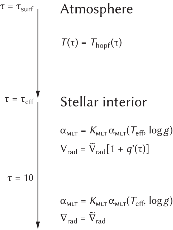
Figure 2: The changes to a garstec stellar structure model as a result of our implementation. In the radiative atmosphere, a different temperature stratification, given by eq. (3), is used and the transition point is altered. In the outer, convective parts of the interior model, the radiative gradient is modified according to eq. (5). Everywhere in the interior of the star, the calibrated $\alpha_{\textup{\tiny MLT}}(T_{\textup{eff}},\log g)$ from eq. (2) is used. In mesa, the stellar interior extends all the way to $\tau_{\textup{surf}}$, but the photospheric quantities are determined at $\tau=\tau_{\textup{eff}}$.

4 Stellar Evolution with 3D results

We have taken much care to adopt as similar as possible microphysics in the stellar evolution code as in the 3D simulations in order to produce a consistent model.

The envelope models which Trampedach et al. (2014b) utilised to perform the 3D $\alpha_{\textup{\tiny MLT}}$-calibration were calculated with the MLT treatment from Böhm-Vitense (1958). To include the calibrated $\alpha_{\textup{\tiny MLT}}$ values, we also use a standard mixing-length theory of convection in our stellar evolution calculations. Strictly speaking, the $\alpha_{\textup{\tiny MLT}}$ calibration is only valid for precisely the same MLT implementation. But it is important to note, that even different MLT-flavors will yield the same temperature evolution, if $\alpha_{\textup{\tiny MLT}}$ is properly calibrated to the Sun (Gough & Weiss, 1976; Pedersen et al., 1990; Salaris & Cassisi, 2008). In mesa the formulation from Cox & Giuli (1968) is employed, while garstec relies on the prescription from Kippenhahn et al. (2012).

As mentioned earlier, the simulations use a non-standard solar mixture. This mixture will be used in garstec, while we for the mesa models settle for the almost identical GN93.

The atmospheric simulations use the Mihalas-Hummer-Däppen (MHD) equation of state (EoS) (Hummer & Mihalas, 1988; Mihalas et al., 1988; Däppen et al., 1988), which we have readily available in garstec, but not in mesa. To span the temperature range necessary for a full structure model, we complement the MHD-EoS with the OPAL-EoS (Rogers & Nayfonov, 2002) in garstec. In mesa we only use OPAL-EoS.

Trampedach et al. (2014a) calculated their own low-temperature opacities for the 3D simulations. In the envelope model used for the $\alpha_{\textup{\tiny MLT}}$-calibration, these were merged with interior opacities from the Opacity Project (OP, Badnell et al., 2005). We have used the available OP data to calculate opacity tables for the quite specific mixture used in the 3D simulations and merged them with the atmospheric opacities from Trampedach et al. (2014a) provided by R. Trampedach (priv. comm.). These custom opacities are used in garstec. In MESA, we instead combine the low-temperature Trampedach-opacities with tables from OPAL (Iglesias & Rogers, 1996). For completeness it should be added that we use the Potekhin conductive opacities (Cassisi et al., 2007).

4.1 Solar calibration

The first step is to calculate a standard solar model (SSM) using our new implementation. This is done by performing a solar calibration, which determines the initial chemical composition and the $\alpha_{\textup{\tiny MLT}}$ scaling factor from eq. (2). Microscopic diffusion – which is required to perform the procedure – is included in all of our models.

A solar calibration with the 3D results activated yields a scaling factor of $K_{\textup{\tiny MLT}}=1.024$ for garstec and $K_{\textup{\tiny MLT}}=1.034$ for mesa. The value of $\alpha_{\textup{\tiny MLT}}$ for the solar simulation in the grid of 3D simulations is $\alpha_{\textup{{\tiny MLT}, grid},\odot}=1.764$; thus, the corresponding values are $\alpha_{\textup{\tiny MLT, }\odot}=1.807$ for garstec and $\alpha_{\textup{\tiny MLT, }\odot}=1.828$ for mesa.

In the following we will compare the models with our new 3D implementation to standard reference models, i.e., evolution with a constant, solar-calibrated $\alpha_{\textup{\tiny MLT}}$ and Eddington grey atmosphere, but otherwise using the same microphysics. When performing these standard Eddington solar calibrations we obtain virtually the same initial abundances as with our 3D implementations. For reference, we get $\alpha_{\textup{\tiny MLT, }\odot}=1.702$ for garstec and $\alpha_{\textup{\tiny MLT, }\odot}=1.672$ for mesa, which is already a clear indication that the outermost structure has changed compared to the 3D case.

4.2 Evolution

After the solar calibration, the first natural test of our new implementation is to calculate evolutionary tracks and compare to reference tracks. This is shown in Fig. 3 and Fig. 4.

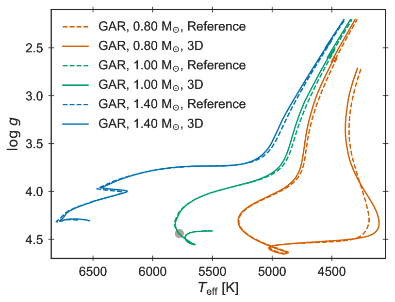
Figure 3: Stellar evolutionary tracks from garstec. The reference-tracks are computed using a constant, solar calibrated $\alpha_{\textup{\tiny MLT}}$ and an Eddington atmosphere. The 3D-tracks use our implementation of variable $\alpha_{\textup{\tiny MLT}}$ and a $T(\tau)$ relation from 3D simulations. To not clutter the plot, the full pre-main sequence phase is only shown for the $0.80\,\text{M}_{\odot}$ track. The present-day Sun is marked in grey.

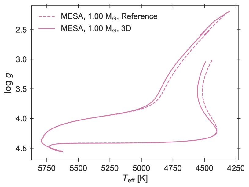
Figure 4: As Figure 3, but calculated with mesa and showing only the $1.00\,\text{M}_{\odot}$ track including the PMS phase. The extrapolation in the RGB is treated differently (details in the text).

From the plots it is clear that the main sequence of the $1.00\,\text{M}_{\odot}$ evolution is nearly identical for the two tracks. This is just as expected, as the solar calibration ensures that both of them go through the same point at the Sun’s age (highlighted in grey in the figure). The turn-off is almost identical as well, with a temperature difference of less than $7\,\text{K}$. The same is the case for the turn-off of the $0.80\,\text{M}_{\odot}$ track, where the tracks differ by $5\,\text{K}$. For the $1.40\,\text{M}_{\odot}$ evolution, the tracks are separated by $35\,\text{K}$ at the leftmost point in the hook.

The two sets of tracks are more clearly distinguished from each other on the pre-main sequence (PMS) and on the red-giant branch (RGB), where convection, and in particular its super-adiabatic parts, are most extended. For the garstec tracks, the temperature difference in the RGB at $\log g=3.2$ between 3D and reference is $25\,\text{K}$ for the $0.80\,\text{M}_{\odot}$ track, $28\,\text{K}$ for $1.00\,\text{M}_{\odot}$, and $29\,\text{K}$ for $1.40\,\text{M}_{\odot}$. At the RGB-bump, the difference is unchanged in the case of $0.80\,\text{M}_{\odot}$, roughly halved for $1.00\,\text{M}_{\odot}$, and reduced to $11\,\text{K}$ for the $1.40\,\text{M}_{\odot}$ track. The RGB-bump for the $1.00\,\text{M}_{\odot}$ mesa tracks differ by $32\,\text{K}$.

As expected, the evolutionary pace of the models is also almost unchanged by our new implementation. At the exhaustion of hydrogen in the core (defined as a central hydrogen content of less than $10^{-5}$), the age difference between the two sets of tracks is less than $0.1\%$ for all of the masses. The maximum age difference for the $1.00\,\text{M}_{\odot}$ evolution is obtained, if we instead define the turn-off in a more observational sense – i.e., where $T_{\textup{eff}}$ reaches its highest value – which yields a change in age of around $2\%$ (or $150\,\text{Myr}$).

From the work by Salaris & Cassisi (2015), the $T(\tau)$ relation is expected to play the largest role in the temperature change (see also Section 5). We find that the variable $\alpha_{\textup{\tiny MLT}}$ plays an important role as well – especially in the RGB. A fixed $\alpha_{\textup{\tiny MLT}}$ makes the two tracks move up the RGB in parallel, i.e., with a constant separation. However, with the 3D implementation, the variations in $\alpha_{\textup{\tiny MLT}}$ as the star evolves will give rise to changes in the slope of the ascent. This is visible from the varying temperature differences along the RGB evolution.

4.2.1 Limitations in the RGB

One clear limitation of the method is the coverage of the grid, and therefore the treatment of the borders is important. If the 3D-implementation is fully switched off when the star leaves the valid grid range, the track will suddenly experience a jump in $\alpha_{\textup{\tiny MLT}}$ as well as a different outer boundary condition, and changes temperature accordingly. To avoid this, we rely on extrapolation just outside the boundaries of the grid, which is especially important in the fully convective PMS phase, where the lower mass tracks will leave the grid very briefly. We have tested this near the boundaries at high $\log g$ for both the hot and cold edge – i.e. for stars with higher/lower mass than the $0.80$-$1.40\,\text{M}_{\odot}$ range – where the transition occurs smoothly.

On the RGB – where extrapolation is required to continue the evolution towards lower $\log g$– the situation is a bit more complicated. From the top right corner of Fig. 4 it can be seen that the 3D-track suddenly cools and crosses the reference track. What is happening is that the track leaves the grid resulting in a fast drop in the value of $\alpha_{\textup{\tiny MLT}}$, which effectively makes the track change to a different adiabat and continue its ascent. Clearly, simple extrapolation from the triangulation does not work properly in this region. What is done instead in garstec is to use the last valid values from the grid – i.e. keeping $\alpha_{\textup{\tiny MLT}}$ and the $T(\tau)$ relation fixed during RGB evolution. This produces a smooth evolution as can be seen from Fig. 3 , but is not to be trusted going high up the RGB.

4.3 Model structure

We now compare the structure of the calibrated solar models with the 3D $\alpha_{\textup{\tiny MLT}}$ and $T(\tau)$ relation, to the reference standard solar models with an Eddington $T(\tau)$ relation and constant solar calibrated $\alpha_{\textup{\tiny MLT}}$. As the implementation only affects the layers above and just below the photosphere, this is where we mainly expect to see changes in the models.

In Fig. 5, the temperature structure in the form of $T(\tau)$ is displayed for the solar models with 3D effects activated from both mesa and garstec. They are compared to the $T(\tau)$ relation from the solar entry in the table from Trampedach et al. (2014a, b). The transition point at $\log\tau\simeq-0.3$ (corresponding to $\tau\simeq 0.5$) is marked for clarity. For reference, the Eddington grey $T(\tau)$ relation– which is anchored at $\tau=2/3$ and therefore differs at the marked photosphere – is also displayed in the figure. The figure clearly shows that both models trace the 3D $T(\tau)$ relation used in the calculation closely in the atmosphere.

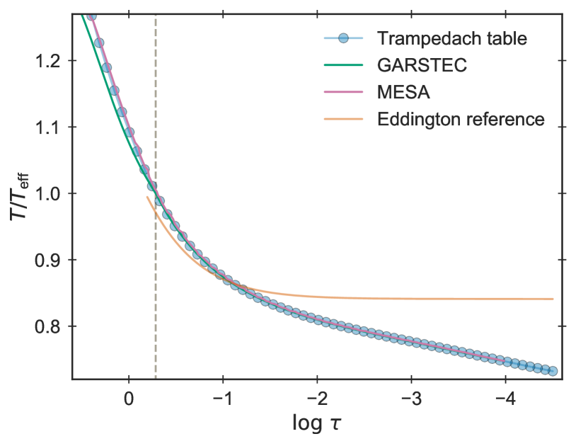
Figure 5: Temperature (normalised to the value at the photosphere) as a function of optical depth in the outermost parts of the garstec and mesa 3D solar models. The grey dashed line marks the photosphere of the stellar structure models. The curve Trampedach table shows the 3D $T(\tau)$ relation of the solar simulation from the table. Finally, the result using an Eddington grey $T(\tau)$ relation is added for reference.

We show the temperature stratification as $T(r)$ for the same solar models in Fig. 6. In this figure, they are compared to the actual structure extracted directly from the 3D simulation of the Sun (provided by R. Trampedach, priv. comm.). It is evident that the models very accurately reproduce the full underlying averaged 3D simulation. Thus, the stellar models are able to recover the actual temperature stratification from the atmosphere simulation. Below the photosphere the models naturally deviate as convection starts to influence the structure, which is also the case in Fig. 5.

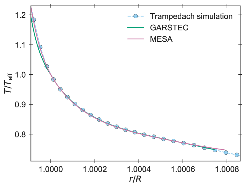
Figure 6: As Fig. 5 but shown as a function of radius (normalised to the photospheric value). The Trampedach simulation is the temperature stratification from the averaged 3D simulation of the Sun from the grid.

4.3.1 Stellar interior

Turning to the interior of the stellar models, we see that the implementation of the 3D results has an insignificant impact on the structure. In general the models are indistinguishable – e.g. with respect to the hydrogen profile. Specifically, the depth of the outer convection zone is left virtually unchanged; the relative difference between 3D and reference is below $0.01\%$ for both mesa and garstec.

4.3.2 Oscillation frequencies

Asteroseismology is an excellent tool for probing the interior of stars, by observing the imprint of the stellar oscillations in the emitted light. The term solar-like oscillations governs stochastically excited waves in stars with an outer convection zone – i.e. stars on the lower main sequence and red giants. The advent of very high quality space-based photometry (from e.g. Kepler) has made it possible to detect such oscillations in distant stars allowing us to gain detailed knowledge of their internal structure (e.g. the review by Chaplin & Miglio, 2013). For stars showing solar-like oscillations, it has revolutionised how well we can determine stellar properties (Lund et al., 2017; Silva Aguirre et al., 2017).

In the present case, we can compare the structure of the calibrated solar models with the observed frequencies from the Sun. We have calculated theoretical oscillation frequencies for our solar models using the Aarhus adiabatic oscillation package (adipls, Christensen-Dalsgaard, 2008). As observations we use solar data from the Birmingham Solar-Oscillation Network (BiSON, Broomhall et al., 2009; Davies et al., 2014). The comparison is shown in Fig. 7 as a difference between the two set of oscillation frequencies for the mesa solar models.

Figure 7: Difference between observed and calculated oscillation frequencies of the Sun. The observations are from BiSON and the model frequencies are from the mesa solar models with and without our modifications.

The general deviation, which increases for higher frequencies, is well-known and expected: it is the asteroseismic surface effect (mentioned in Section 2.1), consequence of the near-surface deficiencies in stellar models. Oscillations of higher and higher frequency probe regions closer and closer to the surface; thus, it is evident from the figure that the two models differ in the surface layers. This is just as anticipated, as the implementation changes the outer boundary condition and the correction from eq. (5) is only applied just below the photosphere (because the optical depth increases very rapidly in the interior). Hence, the inclusion of the 3D effects shifts the oscillation frequencies, which is a known effect of changing the atmospheric structure (e.g. Morel et al., 1994). The frequencies are decreased, thus seemingly bringing the model closer to the observations.

The surface effect can be further improved on by fully replacing the outer layers of the model with an averaged 3D simulation in a so-called patched model (see Section 2.1 and references therein). However, this is (currently) only performed as a final step after the stellar evolution calculation; it is not possible to perform the procedure along the way during the evolution. Furthermore, a full treatment of the surface effect would additionally involve the inclusion of the modal effects, i.e. the effects of nonadiabaticity and the full interaction between convection and pulsations (e.g. Houdek et al., 2017), as is also evident from the results of patched models (e.g Rosenthal et al., 1999; Sonoi et al., 2015; Ball et al., 2016; Jørgensen et al., 2017).

5 Comparison to earlier work

An analysis similar to the one we present in this paper was carried out by Salaris & Cassisi (2015, hereafter SC15) using the stellar evolution code BaSTI (BAg of Stellar Tracks and Isochrones, Pietrinferni et al., 2004). They implemented the same 3D results, namely the calibrated $\alpha_{\textup{\tiny MLT}}$ and $T(\tau)$ relations from Trampedach et al. (2014a, b). However, the description of their implementation is brief and differs from ours in a few ways.

One central topic is the transition point between atmosphere and stellar interior, and the location of the photosphere in the model. SC15 used a constant $\tau_{\textup{fit}}=2/3$ as transition point (and mention that they have tested various other values down to $\tau_{\textup{fit}}=100$). The crucial matter is not the exact value, but whether this transition point has been used as the photosphere in the stellar model or not. The optical depth $\tau_{\textup{eff}}$ in the 3D $T(\tau)$ relation at which $T=T_{\textup{eff}}$ varies, but is always close to $\tau_{\textup{eff}}\simeq 0.5$. As argued earlier in Section 3.2.1, it will produce a slightly inconsistent model, if the global ‘photospheric quantities’ (e.g. $T_{\textup{eff}}$ and $\log g$) are still determined at the usual $\tau_{\textup{fit}}=2/3$ or another $\tau_{\textup{fit}}\neq\tau_{\textup{eff}}$. We have taken great care in this respect, either by making sure the transition happens at the correct $\tau_{\textup{fit}}=\tau_{\textup{eff}}$ each time (garstec) or by properly determining the global quantities at this point (mesa).

SC15 mention the use of Trampedach et al. (2014a, eq. (35), (36)) to correct the temperature gradients. First of all, as explained earlier, it is only necessary to apply a correction to the radiative temperature gradient $\nabla_{\textup{rad}}$ (by using eq. (35) from Trampedach et al. (2014a)); the MLT calculation with this modified gradient as input will ensure a properly corrected $\nabla$ without further modifications (R. Trampedach, priv. comm.). Secondly, SC15 find the corrections to be minuscule . We agree for higher values of $\tau$, but just below the photosphere the correction term in eq. (5) is significant – e.g. for the solar models, the temperature gradient is changed by around $20\%$ at $\tau\simeq 1$. A plot of the correction is shown in Appendix C.

As argued earlier – and also by Ludwig et al. (1999) and Trampedach et al. (2014b) – it is appropriate to introduce a calibrated scaling factor instead of using $\alpha_{\textup{\tiny MLT}}$ directly as supplied from the grid. SC15 mention such a scaling as required to produce a standard solar model (see below). However, they did not employ this $\alpha_{\textup{\tiny MLT}}$ scaling factor in their stellar evolution calculations.

5.1 Results

A general difference between our work and SC15 is the focus of the investigation. SC15 did calculate models utilising both the 3D $\alpha_{\textup{\tiny MLT}}$ and $T(\tau)$ relation, but also analysed them separately in order to isolate the impact of the 3D $\alpha_{\textup{\tiny MLT}}$ and $T(\tau)$ relation, respectively. We choose to follow the advice of the original work by Trampedach et al. (2014b), who stress the importance of always employing the extracted results together (as well as using them alongside the corresponding atmospheric opacities).

For their comparison tracks (with different $T(\tau)$ relations), SC15 used the $\alpha_{\textup{\tiny MLT, }\odot}$ from the 3D RHD solar simulation directly, instead of a traditional solar calibrated value. We have chosen to make solar calibrations for both the 3D and reference Eddington case separately, in order to show the difference between using the 3D results and what “modellers usually do”. Thus, a direct comparison of our results to SC15 is not possible. For example, in SC15 the Eddington tracks are generally hotter than the 3D ones while we see the opposite behaviour. Looking at figure 3 in SC15, this is an effect of the choice to not individually calibrate the reference tracks to the Sun in SC15; the main-sequence evolution of the $1.00\,\text{M}_{\odot}$ Eddington track is significantly hotter than the 3D counterpart, where our tracks basically coincide. If we perform evolutionary calculations with similar assumptions – i.e. disable scaling of $\alpha_{\textup{\tiny MLT}}$ for the 3D case, and for the reference case directly use the $\alpha_{\textup{\tiny MLT, }\odot}$ from the grid instead of a solar-calibrated value – we obtain results which are very similar to SC15 (see Appendix B).

SC15 briefly analyse the impact on the standard solar model (SSM) and state that they “find it necessary to rescale the RHD $\alpha_{\textup{\tiny MLT}}$ calibration by a factor of just $1.034$ to reproduce the solar radius”. This is exactly the same we find for the mesa 3D solar calibration and very close to our garstec value. However, this scaling factor was not used to calculate their evolutionary tracks. They do not dig deeper into the interior structure of the SSM, so we are unable to compare our asteroseismic analysis to their work.

6 Conclusions

We have consistently implemented results extracted from 3D radiation-coupled hydrodynamics simulations of stellar convection in the stellar evolution codes garstec and mesa. The new implementation consists of a temperature stratification in the form of $T(\tau)$ relations and corresponding corrected temperature gradients, and a calibrated, variable mixing-length parameter $\alpha_{\textup{\tiny MLT}}(T_{\textup{eff}},\log g)$. We have presented a very detailed account of our implementations, and compared to the earlier implementation of the same 3D results in a stellar evolution code by Salaris & Cassisi (2015). Moreover we make our mesa implementation freely available (see the appendix).

We calculate the evolution of different low-mass stars after a solar calibration. We compare to a set of reference models which uses an Eddington grey atmosphere and constant solar-calibrated $\alpha_{\textup{\tiny MLT}}$. In the pre-main sequence and in the red-giant branch we see the largest effect of the 3D implementation on the temperature evolution. Regarding the evolutionary speed, we see no significant change in the age of the models at core hydrogen exhaustion.

Furthermore, we compare the model structure of the calibrated solar models and see no significant changes. For the first time we present an helioseismic analysis of a standard solar model with a $T(\tau)$ relation and variable $\alpha_{\textup{\tiny MLT}}$ extracted from 3D simulations. The use of the 3D effects makes a small, positive impact on the asteroseismic surface effect.

We note that the method is limited by the coverage in parameter space of the grid of 3D simulations. To make this method widely applicable, an extended coverage in terms of $\log g$ and $T_{\textup{eff}}$ is required, but more importantly: simulations of varying metallicity. One option in this respect would be to extract similar information from the stagger-grid by Magic et al. (2013).

The future aim is to exploit the concept of patched models – which provide a more realistic structure but is static – with the current dynamic approach, to allow for the evolution of more realistic models. Our implementation is one step further along that path and the work by Jørgensen et al. (2017) another. The ultimate goal is to facilitate on-the-fly patching of 3D simulations as outer boundary conditions for stellar evolution calculations.

Appendix A Technical details of the mesa implementation

The opacity tables, $T(\tau)$ relation and mixing-length parameters $\alpha_{\textup{\tiny MLT}}$ for the simulations by Trampedach et al. (2013, 2014a, 2014b) are available from the MESA marketplace as an archive that should be extracted over an existing installation of mesa revision 9575. Code to use the $T(\tau)$ relation in mesa runs is provided in two examples in a new folder hydro_Ttau_examples: calibrate_hydro_Ttau and evolve_hydro_Ttau. The archive also includes code for the equivalent ‘reference” runs with an Eddington grey atmosphere. These are in the folders calibrate_edd and evolve_edd.

The first example, calibrate_hydro_Ttau, provides an example case that was used to calibrate the scaling factor presented in Sec. 4.1. It implements a solar calibration using the astero module, with a small Python script that optimizes the model parameters. This example can be adapted by users wishing to use the 3D $T(\tau)$ relation alongside the astero module. The second example, evolve_hydro_Ttau, provides an example used to compute the evolutionary track presented in Sec. 4.2, and can be adapted for normal evolutionary calculations. In both examples, the code that interpolates the 3D $T(\tau)$ relation and MLT parameters $\alpha_{\textup{\tiny MLT}}$ and modifies the boundary conditions and radiative gradient is included in the files run_star_extras.f and 624.dek. The code for these two examples is also now part of the main mesa codebase and will appear in the test suite of mesa next public release (after r10398). Because of small changes elsewhere in mesa, the results of those test cases are not identical to the results presented here.

A.1 Modification of radiative gradient

Since revision 9575, MESA has included a “porosity” factor $\phi$ that reduces the opacity. By default, when $\phi>1$, the opacity $\kappa$ is replaced by $\kappa/\phi$ when computing the radiative gradient, so the radiative gradient $\nabla_{\textup{rad}}$ is replaced by $\nabla_{\textup{rad}}/\phi$. To modify the radiative gradient as in eq. (5), we therefore assign

$$\phi=\frac{1}{1+q^{\prime}(\tau)}\;,$$ (6)

where $q(\tau)$ has been extracted as described in Sec. 3. It is important to note that the changes to the porosity factor do not currently affect the optical depth $\tau$. If this should change in subsequent versions of MESA, the current implementation will no longer be valid.

In the main codebase for mesa r9575, the porosity factor is hardcoded to have a minimum value of unity. In the $q(\tau)$ given by Trampedach et al. (2014a), this would limit us to $q^{\prime}(\tau)<0$, so our archive includes modified versions of core source files (hydro_eqns.f90 and mlt_info.f90 in star/private) that lift this restriction on the porosity factor. The restriction is also lifted in public releases after r10398 by the creation of a user control for the porosity limit.

A.2 Boundary conditions

With the outermost meshpoint located above the photosphere, mesa needs new outer boundary conditions. We choose these to correspond to an Eddington grey atmosphere evaluated at the optical depth of the outermost meshpoint. For the gas pressure $P_{g}$, we therefore have

$$P_{g} =\left(\frac{g}{\kappa}-\frac{F}{c}\right)\tau$$

$$=\left(\frac{g}{\kappa}-\frac{L}{4\pi R^{2}c}\right)\tau$$

$$=\left(\frac{g}{\kappa}-\frac{Lg}{4\pi GMc}\right)\tau\;,$$ (7)

where $g$ is the gravity, $\kappa$ the Rosseland mean opacity, $F$ the radiative flux, $c$ the speed of light, $\tau$ the optical depth, $R$ the radius at the outermost point, $G$ the gravitational constant and $M$ the total mass of the star.

For the radiation pressure $P_{r}$, we have

$$P_{r} =\frac{1}{3}aT^{4}$$

$$=\frac{4\sigma}{3c}\cdot\frac{3}{4}T_{\textup{eff}}^{4}(\tau+q(\tau))$$

$$=\frac{L}{4\pi R^{2}c}(\tau+q(\tau))$$

$$=\frac{Lg}{4\pi GMc}(\tau+q(\tau))\;,$$ (8)

where $a$ is the radiation constant, $T$ the temperature, $\sigma$ the Stefan-Boltzmann constant, $T_{\textup{eff}}$ the effective temperature and $q$ the Hopf function (see eq. 1).

The total pressure $P$ at the outermost meshpoint is therefore

$$P(\tau)=P_{g}(\tau)+P_{r}(\tau) =\frac{g}{\kappa}\tau+\frac{Lg}{4\pi GMc}q(\tau)$$

$$=\frac{g}{\kappa}{\tau}\left[1+\frac{\kappa}{\tau}\frac{L}{4\pi GMc}q(\tau)\right]\;.$$ (9)

These are, in effect, equivalent to the initial conditions that mesa uses when integrating an atmosphere from small optical depths down to the photosphere to obtain photospheric boundary conditions.

Appendix B Models with SC15 settings

Here we present models calculated with garstec utilising similar settings as those used by SC15 (i.e. Salaris & Cassisi, 2015). The 3D case is calculated without scaling of $\alpha_{\textup{\tiny MLT}}$, i.e. just by adopting the values directly from the grid. The reference Eddington tracks do not rely on a solar calibrated $\alpha_{\textup{\tiny MLT}}$, but rather the value $\alpha_{\textup{\tiny MLT, }\odot}$ directly from the solar 3D simulation. Moreover, the tracks are calculated with the GN93 composition and without diffusion. The resulting tracks for the $1\,\text{M}_{\odot}$ star can be seen in Fig. 8, which is very similar to the corresponding track in figure 3 of SC15. The figure can also be compared to our models in Fig. 3 and Fig. 4.

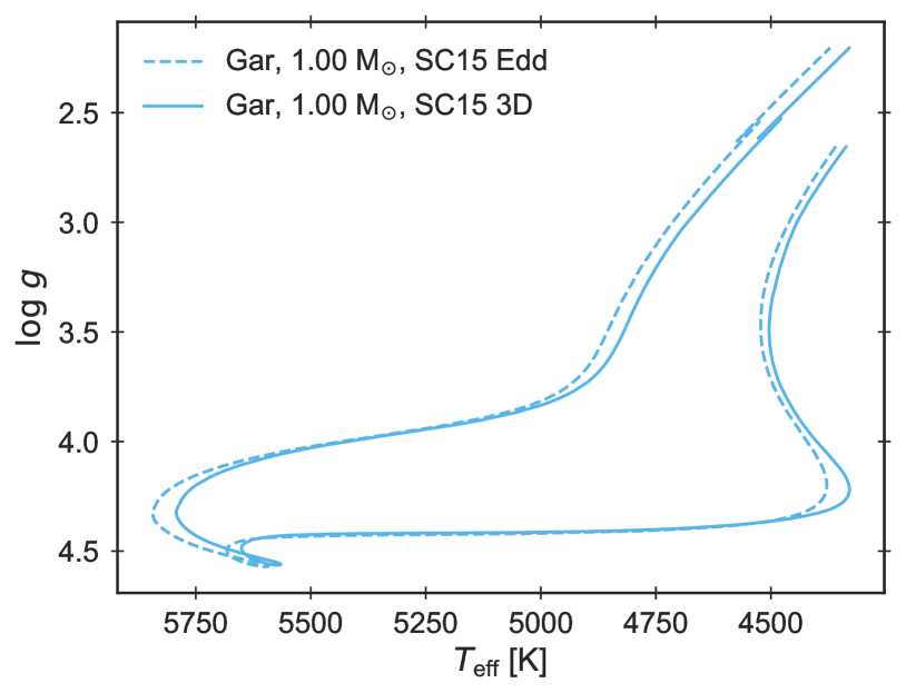
Figure 8: Stellar evolution calculated with garstec using same settings as SC15 (see text for details).

Appendix C Correction of the gradients

In this appendix we highlight the impact of the correction factor in eq. (5) on the temperature gradients. The result from the mesa solar model as well as $1+q^{\prime}(\tau)$ derived directly from the Trampedach data table is shown in Fig. 9 in the region near the photosphere. It is clear that the changes are significant around the photosphere and quickly decrease going into the star – and that the model accurately reproduce the table.

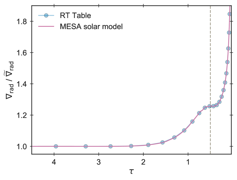
Figure 9: Magnitude of the correction term in eq. (5) for the mesa solar model and derived directly from the table of 3D results. The grey dashed line marks the photosphere at $\tau_{\textup{eff}}\simeq 0.5$.

References

- Akima (1970) Akima H., 1970, Journal of the ACM, 17, 589
- Akima (1991) Akima H., 1991, ACM Transactions on Mathematical Software, 17, 341
- Anders & Grevesse (1989) Anders E., Grevesse N., 1989, Geochimica et Cosmochimica Acta, 53, 197
- Badnell et al. (2005) Badnell N. R., Bautista M. A., Butler K., Delahaye F., Mendoza C., Palmeri P., Zeippen C. J., Seaton M. J., 2005, Monthly Notices of the Royal Astronomical Society, 360, 458
- Ball et al. (2016) Ball W. H., Beeck B., Cameron R. H., Gizon L., 2016, Astronomy & Astrophysics, 592, A159
- Böhm-Vitense (1958) Böhm-Vitense E., 1958, Zeitschrift für Astrophysik, 46
- Borucki et al. (2010) Borucki W. J., et al., 2010, Science, 327, 977
- Broomhall et al. (2009) Broomhall A.-M., Chaplin W. J., Davies G. R., Elsworth Y., Fletcher S. T., Hale S. J., Miller B., New R., 2009, Monthly Notices of the Royal Astronomical Society: Letters, 396, L100
- Brown (1984) Brown T. M., 1984, Science, 226, 687
- Cassisi et al. (2007) Cassisi S., Potekhin A. Y., Pietrinferni A., Catelan M., Salaris M., 2007, The Astrophysical Journal, 661, 1094
- Chaplin & Miglio (2013) Chaplin W. J., Miglio A., 2013, Annual Review of Astronomy and Astrophysics, 51, 353
- Christensen-Dalsgaard (2008) Christensen-Dalsgaard J., 2008, Astrophysics and Space Science, 316, 113
- Christensen-Dalsgaard et al. (1988) Christensen-Dalsgaard J., Däppen W., Lebreton Y., 1988, Nature, 336, 634
- Cline & Renka (1984) Cline A. K., Renka R. L., 1984, Rocky Mountain Journal of Mathematics, 14, 119
- Cox & Giuli (1968) Cox J. P., Giuli R. T., 1968, Principles of Stellar Structure. New York: Gordon and Breach
- Däppen et al. (1988) Däppen W., Mihalas D., Hummer D. G., Mihalas B. W., 1988, The Astrophysical Journal, 332, 261
- Davies et al. (2014) Davies G. R., Broomhall A.-M., Chaplin W. J., Elsworth Y., Hale S. J., 2014, Monthly Notices of the Royal Astronomical Society, 439, 2025
- Gough & Weiss (1976) Gough D. O., Weiss N. O., 1976, Monthly Notices of the Royal Astronomical Society, 176, 589
- Grevesse & Noels (1993) Grevesse N., Noels A., 1993, in Hauck B., Paltani S., Raboud D., eds, Perfectionnement de l’Association Vaudoise des Chercheurs en Physique. pp 205–257
- Hjørringgaard et al. (2017) Hjørringgaard J. G., Silva Aguirre V., White T. R., Huber D., Pope B. J. S., Casagrande L., Justesen A. B., Christensen-Dalsgaard J., 2017, Monthly Notices of the Royal Astronomical Society, 464, 3713
- Houdek et al. (2017) Houdek G., Trampedach R., Aarslev M. J., Christensen-Dalsgaard J., 2017, Monthly Notices of the Royal Astronomical Society: Letters, 464, L124
- Hummer & Mihalas (1988) Hummer D. G., Mihalas D., 1988, The Astrophysical Journal, 331, 794
- Huynh (1993) Huynh H. T., 1993, SIAM Journal on Numerical Analysis, 30, 57
- Iglesias & Rogers (1996) Iglesias C. A., Rogers F. J., 1996, The Astrophysical Journal, 464, 943
- Jørgensen et al. (2017) Jørgensen A. C. S., Weiss A., Mosumgaard J. R., Silva Aguirre V., Sahlholdt C. L., 2017, Monthly Notices of the Royal Astronomical Society, 472, 3264
- Kippenhahn et al. (2012) Kippenhahn R., Weigert A., Weiss A., 2012, Stellar Structure and Evolution, 2nd edn. Springer-Verlag Berlin Heidelberg
- Krishna Swamy (1966) Krishna Swamy K. S., 1966, The Astrophysical Journal, 145, 174
- Li et al. (2018) Li T., Bedding T. R., Huber D., Ball W. H., Stello D., Murphy S. J., Bland-Hawthorn J., 2018, Monthly Notices of the Royal Astronomical Society, 475, 981
- Ludwig et al. (1999) Ludwig H.-G., Freytag B., Steffen M., 1999, Astronomy & Astrophysics, 346, 111
- Lund et al. (2017) Lund M. N., et al., 2017, The Astrophysical Journal, 835, 172
- Magic & Weiss (2016) Magic Z., Weiss A., 2016, Astronomy & Astrophysics, 592, A24
- Magic et al. (2013) Magic Z., Collet R., Asplund M., Trampedach R., Hayek W., Chiavassa A., Stein R. F., Nordlund Å., 2013, Astronomy & Astrophysics, 557, A26
- Mihalas et al. (1988) Mihalas D., Dappen W., Hummer D. G., 1988, The Astrophysical Journal, 331, 815
- Morel et al. (1994) Morel P., van’t Veer C., Provost J., Berthomieu G., Castelli F., Cayrel R., Goupil M. J., Lebreton Y., 1994, Astronomy and Astrophysics, 286, 91
- Mosumgaard et al. (2017) Mosumgaard J. R., Silva Aguirre V., Weiss A., Christensen-Dalsgaard J., Trampedach R., 2017, in Monteiro M., Cunha M., Ferreira J., eds, EPJ Web of Conferences Vol. 160, Seismology of the Sun and the Distant Stars II. p. 03009
- Nordlund et al. (2009) Nordlund Å., Stein R. F., Asplund M., 2009, Living Reviews in Solar Physics, 6
- Paxton et al. (2011) Paxton B., Bildsten L., Dotter A., Herwig F., Lesaffre P., Timmes F., 2011, ApJS, 192, 3
- Paxton et al. (2013) Paxton B., et al., 2013, ApJS, 208, 4
- Paxton et al. (2015) Paxton B., et al., 2015, ApJS, 220, 15
- Pedersen et al. (1990) Pedersen B. B., Vandenberg D. A., Irwin A. W., 1990, The Astrophysical Journal, 352, 279
- Piau et al. (2014) Piau L., Collet R., Stein R. F., Trampedach R., Morel P., Turck-Chièze S., 2014, Monthly Notices of the Royal Astronomical Society, 437, 164
- Pietrinferni et al. (2004) Pietrinferni A., Cassisi S., Salaris M., Castelli F., 2004, The Astrophysical Journal, 612, 168
- Rogers & Nayfonov (2002) Rogers F. J., Nayfonov A., 2002, The Astrophysical Journal, 576, 1064
- Rosenthal et al. (1999) Rosenthal C. S., Christensen-Dalsgaard J., Nordlund Å., Stein R. F., Trampedach R., 1999, Astronomy and Astrophysics, 351, 689
- Salaris & Cassisi (2008) Salaris M., Cassisi S., 2008, Astronomy & Astrophysics, 487, 1075
- Salaris & Cassisi (2015) Salaris M., Cassisi S., 2015, Astronomy & Astrophysics, 577, A60
- Salaris et al. (2002) Salaris M., Cassisi S., Weiss A., 2002, Publications of the Astronomical Society of the Pacific, 114, 375
- Salaris et al. (2018) Salaris M., Cassisi S., Schiavon R. P., Pietrinferni A., 2018, A&A, 612, A68
- Silva Aguirre et al. (2017) Silva Aguirre V., et al., 2017, The Astrophysical Journal, 835, 173
- Sonoi et al. (2015) Sonoi T., Samadi R., Belkacem K., Ludwig H.-G., Caffau E., Mosser B., 2015, Astronomy & Astrophysics, 583, A112
- Stein & Nordlund (1989) Stein R. F., Nordlund Å., 1989, The Astrophysical Journal, 342, L95
- Stein & Nordlund (1998) Stein R. F., Nordlund Å., 1998, The Astrophysical Journal, 499, 914
- Suresh & Huynh (1997) Suresh A., Huynh H. T., 1997, Journal of Computational Physics, 136, 83
- Tanner et al. (2014) Tanner J. D., Basu S., Demarque P., 2014, The Astrophysical Journal, 785, L13
- Tayar et al. (2017) Tayar J., et al., 2017, The Astrophysical Journal, 840, 17
- Trampedach et al. (2013) Trampedach R., Asplund M., Collet R., Nordlund Å., Stein R. F., 2013, The Astrophysical Journal, 769, 18
- Trampedach et al. (2014a) Trampedach R., Stein R. F., Christensen-Dalsgaard J., Nordlund Å., Asplund M., 2014a, Monthly Notices of the Royal Astronomical Society, 442, 805
- Trampedach et al. (2014b) Trampedach R., Stein R. F., Christensen-Dalsgaard J., Nordlund Å., Asplund M., 2014b, Monthly Notices of the Royal Astronomical Society, 445, 4366
- Trampedach et al. (2017) Trampedach R., Aarslev M. J., Houdek G., Collet R., Christensen-Dalsgaard J., Stein R. F., Asplund M., 2017, Monthly Notices of the Royal Astronomical Society, 466, L43
- Vernazza et al. (1981) Vernazza J. E., Avrett E. H., Loeser R., 1981, The Astrophysical Journal Supplement Series, 45, 635
- Weiss & Schlattl (2008) Weiss A., Schlattl H., 2008, Astrophysics and Space Science, 316, 99
- White et al. (2017) White T. R., et al., 2017, Astronomy & Astrophysics, 601, A82