Quantum dynamics with stochastic reset

Abstract

We study non-equilibrium dynamics of integrable and non-integrable closed quantum systems whose unitary evolution is interrupted with stochastic resets, characterized by a reset rate $r$, that project the system to its initial state. We show that the steady state density matrix of a non-integrable system, averaged over the reset distribution, retains its off-diagonal elements for any finite $r$. Consequently a generic observable $\hat{O}$, whose expectation value receives contribution from these off-diagonal elements, never thermalizes under such dynamics for any finite $r$. We demonstrate this phenomenon by exact numerical studies of experimentally realizable models of ultracold bosonic atoms in a tilted optical lattice. For integrable Dirac-like fermionic models driven periodically between such resets, the reset-averaged steady state is found to be described by a family of generalized Gibbs ensembles (GGE s) characterized by $r$. We also study the spread of particle density of a non-interacting one-dimensional fermionic chain, starting from an initial state where all fermions occupy the left half of the sample, while the right half is empty. When driven by resetting dynamics, the density profile approaches at long times to a nonequilibrium stationary profile that we compute exactly. We suggest concrete experiments that can possibly test our theory.

I Introduction

Non-equilibrium dynamics of closed quantum systems has been a subject of intense theoretical and experimental studies in recent years [rev1, ; rev2, ; rev3, ; rev4, ; rev5, ]. The initial theoretical endeavor in this direction focussed on the study of ramps and quenches through quantum critical points and surfaces [subir0, ; pascal1, ; kibble1, ; zureck1, ; anatoly1, ; ks1, ; ks2, ; ks3, ; degrandi1, ; sumit1, ]. The former class of studies investigated the excitation density and residual energies of a quantum system after a ramp. In the presence of a quantum critical point or surface which is traversed during the ramp, such quantities exhibit power law variation with the ramp rate with universal exponents [rev1, ; kibble1, ; zureck1, ; anatoly1, ; ks1, ; ks2, ; ks3, ; degrandi1, ; sumit1, ]. The study of long-time behavior of quantum systems after a sudden quench and the nature of the resultant steady states (provided they exist) have been some of the central issues addressed in the latter class of studies [subir0, ; pascal1, ; degrandi1, ; rev5, ].

It is well-known that the nature of these steady states depends on whether such systems are integrable. The dynamics of integrable systems is typically non-ergodic due to the presence of large number of quasi-local conserved quantities $Q_{i}$. The presence of such conserved quantities implies that integrable systems, taken out of equilibrium, relax to steady states whose precise form depend on $Q_{i}$. The density matrix describing such steady states may be expressed as $\rho\sim\exp[-\sum_{i}\lambda_{i}Q_{i}]$, where the parameters $\lambda_{i}$ are determined from initial values of $Q_{i}$ [rev1, ; rev5, ]. Such a form of the steady state density matrix follows from entropy maximization in the presence of the conserved quantities $Q_{i}$. The corresponding ensemble is termed as generalized Gibbs ensemble (GGE)[rev1, ].

In contrast, for non-integrable systems, one typically reaches a thermal distribution at late times where the system is described by a diagonal density matrix with an effective temperature [mrigol1, ; mrigol2, ; rev5, ]. In these thermal steady states, the expectation value of any typical local observable $\hat{O}$ of the system is expected to agree with that obtained by averaging over a microcannonical ensemble. The above-mentioned feature can be viewed as a consequence of the eigenstate thermalization hypothesis(ETH). This hypothesis follows from the fact that for a generic quench protocol, the post-quench dynamics of any state with fixed initial energy $\epsilon$ is governed by the final Hamiltonian. Thus such dynamics preserves $\epsilon$. The system under such dynamics explores all eigenstates in the vicinity of $\epsilon$. Since such dynamics is ergodic over all eigenstates within a narrow energy shell of $\epsilon$ and $\epsilon+\delta\epsilon$, the time average of any observable can be equated to the microcanonical ensemble average over these states: $\langle m|\hat{O}|n\rangle\simeq O_{\rm mc}(\bar{\epsilon})\delta_{mn}$. Here $\bar{\epsilon}=(\epsilon_{m}+\epsilon_{n})/2$ and $O_{\rm mc}={\rm Tr}[\rho_{\rm mc}(\bar{\epsilon})\hat{O}]$ is the expectation value of $\hat{O}$ as obtained from a microcannonical ensemble with energy $\bar{\epsilon}$. ETH then states that the difference of $\langle m|\hat{O}|n\rangle$ from $O_{\rm mc}(\bar{\epsilon})$ must vanish in the thermodynamic limit [mrigol1, ; mrigol2, ; srednicci1, ; rev5, ].

More recently, the study of such long-time behavior for periodically driven systems has also been undertaken [rev1, ; arnabd1, ; asen0, ]. It is well-known that for non-integrable systems a periodic drive heats up the system and takes it to an infinite temperature fixed point. However, for integrable models this is not the case, and periodically driven integrable systems may exhibit novel steady states [arnabd1, ]. The behavior of such systems in the presence of a stochastic aperiodicity superposed over a periodic drive has also been studied recently [asen0, ].

In a different classical context, a number of recent studies have found that a classical system evolving under its own natural dynamics, when interrupted stochastically at random times following which the system is reset to its initial condition, evolves at long times into a nontrivial nonequilibrium stationary state [EM12011, ; EM22011, ; EM32014, ; GMS2014, ; DHP2014, ; MSS2015, ; MSS22015, ; Pal2015, ; EM2016, ; NG2016, ; BEM2016, ; PKE2016, ; FBGM2017, ; MT2017, ; RG2017, ]. This is most easily seen in the case of a single diffusive particle on a line, starting at $x=0$. The position of a particle at time $t$, without any resetting, has the standard probability density $P(x,t)=e^{-x^{2}/{4Dt}}/\sqrt{4\pi Dt}$ at time $t$, where $D$ is the diffusion constant. If the particle is now reset to $x=0$ after a random exponentially distributed time with rate $r$, the probability density at long times becomes time-independent [EM12011, ; EM22011, ] and is given by: $P_{\rm stat}(x)=(\alpha_{0}/2)\,\exp[-\alpha_{0}\,|x|]$, with $\alpha_{0}=\sqrt{r/D}$. This result generalizes easily to higher dimensions [EM32014, ]. The approach to this stationary state was shown to have an unusual relaxation dynamics, accompanied by a dynamical phase transition [MSS2015, ]. Such resetting dynamics also has important consequences for search processes: instead of searching for a target by pure diffusion, it is more efficient to reset the searcher at its initial position at random times—a lot of recent studies have demonstrated this in a number of classical systems by studying the associated first-passage problems [Rednerbook, ; BMSreview, ] in the presence of resetting [EM12011, ; EM22011, ; EMM2013, ; WEM2013, ; MV2013, ; KMSS2014, ; RUK2014, ; CS2015, ; R2016, ; BBS2016, ; MPV2017, ; PR2017, ]. Functionals of Brownian motion with resetting have also been studied recently [MST2015, ; HT2017, ; HMMT2018, ]. Another interesting observation is how resetting leads to novel stochastic thermodynamics and the associated fluctuation theorems in classical systems [FGS2016, ; PR22017, ]. In addition, quantum systems with projective measurements have been studied in the context of fluctuation theorems and statistics of energy transfer between the system and the measurement apparatus [sto1, ]. Moreover, there have been several recent studies on quantum first detection problems which involves interrupting unitary evolution of a quantum system with projective measurements [dhar1, ; eli1, ]. However, the analog of a nonequilibrium stationary state induced by random resettings is yet to be explored, to the best of our knowledge, for closed quantum systems that undergo unitary evolution in the absence of resetting.

In this work, we study the dynamics of integrable and non-integrable quantum systems whose unitary evolution is interrupted by stochastic resets, characterized by a reset rate $r$. We consider each reset to project the wavefunction of the system to its initial value at $t=0$. For a perfect reset protocol, which is what we shall be mostly concerned with in this work, this is done with unit probability. The main results obtained from our study of dynamics with stochastic resets are as follows.

First, for non-integrable systems, we consider a generic initial state which is not an eigenstate of the Hamiltonian controlling its unitary evolution. We study the evolution of this state in the presence of a stochastic reset characterized by rate $r$. We demonstrate that such dynamics leads to a reset averaged steady state density matrix (provided such a steady state exists for unitary evolution without reset) which retains its off-diagonal elements. Thus such systems are not described by a diagonal density matrix in their steady states. Consequently, the expectation value of a typical observable does not reduce to its thermal steady state value under such dynamics. Our result reproduces the diagonal density matrix for the steady state for $r=0$ which coincides with known results for standard unitary evolution of a quantum system [rev5, ]. In addition, it also leads to the quantum Zeno effect for $r\to\infty$ [zenoref, ]; in such a situation, the initial state does not evolve and the density matrix of the system is same as the initial density matrix at $t=0$.

Second, for studying the reset dynamics of integrable systems we consider two distinct models. The first of these constitutes a system of free fermions occupying the left half of a one dimensional (1D) chain at $t=0$. These fermions evolve under a nearest-neighbor hopping Hamiltonian [antal1, ; antal2, ; eisler1, ]. We show that interruption of the unitary evolution of these fermions with stochastic reset leads to non-trivial modification of their reset averaged density, $n_{m}(r)$, where $m$ is the site index and $r$ is the reset rate. We also find an exact scaling function for $n_{m}(r)$ and show that it reproduces the known behavior of $n_{m}$ for $r=0$ and $r\to\infty$. The second model involves a periodically driven Dirac Hamiltonian in $d$-dimensions whose unitary evolution is interrupted by a reset after a random integer number of periods. The unitary dynamics of such a Hamiltonian is controlled by a periodic drive characterized by a time period $T$. We show that the reset averaged steady state of such driven systems correspond to GGEs characterized by a reset rate $r$. We demonstrate this by computing non-trivial correlation functions of the model. We find that the steady state values of these correlation functions, averaged over the reset probability, are smooth functions of $r$ which demonstrates the $r$ dependence of the underlying GGEs.

Third, we carry out exact numerical studies of post-quench dynamics of experimentally realizable models of ultracold bosonic atoms in a tilted optical lattice in the presence of resets. The low-energy physics of these bosons can be described in terms of dipoles (bound pair of bosons and holes)[subir1, ; greiner1, ; greiner2, ]. We show that the excitation density of these dipoles $n_{d}$, the dipole density-density correlation function $C$, and the half-chain entanglement entropy $S$ of the boson chain, averaged over the reset probability distribution, interpolates continually between their values of reset free dynamics ($r=0$) and the quantum Zeno limit ($r\to\infty$). We discuss experiments in context of this boson model which can test our theory.

The plan of the rest of the work is as follows. In Sec. II, we present the general formalism for time evolution with reset for generic non-integrable quantum systems and demonstrate that the resultant steady state density matrix, averaged over reset probability, retains its off-diagonal elements for any finite $r$. This is followed by Sec. III where we discuss the dynamics of integrable models, namely, the 1D fermion chain and the $d$-dimensional Dirac fermions, under such reset. In Sec. IV, we address the dynamics of the Bose-Hubbard model in a tilted optical lattice in the presence of stochastic reset. Finally, we chart out experiments which test our theory, discuss our main results, and conclude in Sec. V. Some applications of quantum dynamics with stochastic resets to single particle quantum mechanical systems are discussed in the Appendix A. Some other details concerning the derivation of a scaling function are provided in Appendix B.

II General Formalism

In this section, we consider a generic non-integrable quantum system with unitary evolution interrupted by stochastic resets. In what follows, we shall first consider the case when the reset takes the system to its initial ground state with unit probability. We shall briefly comment on the case of imperfect resets (where the state of system may projected to some other states with a small but non-zero probability) later in this section.

The time evolution of our system is defined precisely as follows. Consider a quantum system, with a given Hamiltonian $H(t)$ (which can in general be time-dependent), prepared initially at $t=0$ in the state $|\psi(0)\rangle$. Now, the state $|\psi(t)\rangle$ evolves from $t$ to $t+dt$ as follows:

$$|\psi(t+dt)\rangle=\begin{cases}|\psi(0)\rangle,\quad\quad\quad\quad\quad\quad{\rm with}\,\,{\rm prob.}\,\,r\,dt\\ \\ [1-iH(t)\,dt]\,|\psi(t)\rangle\,\,\,\,{\rm with}\,\,{\rm prob.}\,\,1-r\,dt\end{cases}$$

where we have set $\hbar=1$ for convenience. Here $r\geq 0$ denotes the reset rate with which the system is projected back to the initial state. Thus, in a small time interval $dt$, the system either goes back to its initial state with probability $r\,dt$, or, with the complementary probability $(1-r\,dt)$, it evolves unitarily with its Hamiltonian $H(t)$. The density matrix ${\hat{\rho}}(t)$ of the system at fixed time $t$, assuming it is in a pure state, is then given by

$${\hat{\rho}}(t)=|\psi(t)\rangle\langle\psi(t)|\,.$$ (1)

Note that for $r=0$, we have a purely unitary evolution and $|\psi(t)\rangle$ is given by

$$|\psi(t)\rangle_{r=0}=U(0,t)\,|\psi(0)\rangle$$ (2)

where the unitary operator is $U$ is given by

$$U(t_{1},t_{2})=T_{t}\,\exp[-i\int_{t_{1}}^{t_{2}}H(t^{\prime})dt^{\prime}],$$ (3)

with $T_{t}$ denoting the time ordering. However for any $r>0$, the dynamics is a mixture of stochastic and deterministic evolution and the density matrix in Eq. (1) is stochastic in the sense that it varies from one realization of the reset process to another. Hence, the observed density matrix at time $t$ is obtained by averaging over all possible reset histories

$$\rho(t)=E\left[{\hat{\rho}}(t)\right]$$ (4)

where $E$ denotes the classical expectation value over all stochastic evolutions. Our goal is to investigate how a nonzero $r$ modifies the time evolution of the quantum state, or equivalently the associated density matrix in Eq. (4). A possible way to realize this mixture of deterministic and stochastic dynamics in Eq. (II) in a realistic system will be discussed later.

To compute the time evolution of the density matrix $\rho(t)$ in Eq. (4) in the presence of a finite resetting rate $r$, we first make the following observation. The resetting protocol essentially induces a renewal process in the sense that after each reset, the system again evolves unitarily from the same initial state without having any memory of what happened before the last reset. Hence, given the observation time $t$, what really matters is how much time has elapsed since the last reset till time $t$. Clearly, this time $\tau$, since the last reset, is a random variable $\tau\in[0,t]$, whose probability density $p(\tau|t)$ (given a fixed observation time $t$) can be estimated as follows. Imagine time running backwards from $t$ and consider the event that there is no reset in the interval $[t-\tau,t]$ followed by a reset in the small time interval $d\tau$. Now, since the resetting is a Poisson process with rate $r$, the probability that there is no reset in $[t-\tau,t]$ is simply $e^{-r\tau}$. The probability of a reset in $d\tau$ is just $r\,d\tau$. Hence, taking the product, the probability of this event is $r\,e^{-r\tau}\,d\tau$. Hence we get

$$p(\tau|t)\,d\tau=r\,e^{-r\tau}\,d\tau\quad\quad 0\leq\tau<t$$ (5)

Integrating, we get

$$\int_{0}^{t}p(\tau|t)d\tau = 1-e^{-rt}$$ (6)

which shows that the pdf $p(\tau|t)$ is not normalized to unity, because the right hand side of Eq. (6) is just the probability that there is at least one reset in $[0,t]$. There is however the possibility of having no reset in $[0,t]$: the probability for this event is simply $e^{-rt}$. Hence, the pdf normalized to unity, given a fixed $t$, can be written as

$$p(\tau|t)=r\,e^{-r\,\tau}+e^{-r\,t}\,\delta(\tau-t)\quad\,0\leq\tau\leq t\,.$$ (7)

It is easy to check that $\int_{0}^{t}p(\tau|t)\,d\tau=1$. The delta function term in Eq. (7) effectively describes the probability of the event of having no reset in $[0,t]$. Note that by making the observation time $t$ large enough we can arbitrarily reduce the probability of zero reset, and get rid of the last term in Eq. (7).

Now let us consider the unitary evolution of the system, following the last reset till the observation time $t$. The density matrix of the system at $t$, given that $\tau$ is the time elapsed since the last reset, is simply

$${\hat{\rho}}(\tau|t) = U(0,\tau)\,\rho_{0}\,U^{\dagger}(0,\tau)$$ (8)

where $U$ is the unitary operator in Eq. (3) and $\rho_{0}$ is the density matrix immediately after the last reset. However, for perfect reset, $\rho_{0}=|\psi(0)\rangle\langle\psi(0)|$ is just the initial density matrix (since the system was projected to the initial state at the last reset). Thus, using Eq. (7) one finds that the density matrix $\rho(t)$ in Eq. (4) (upon averaging over the random variable $\tau$ associated with the reset process) is given by

$$\rho(t) = \int_{0}^{t}re^{-r\tau}\,\rho(\tau|t)\,d\tau$$ (9)

$$+e^{-rt}\,U(0,t)\,\rho_{0}\,U^{\dagger}(0,t)$$

where the last term corresponds to the event that there is no reset within $[0,t]$. Now, at long times $t$, this last term vanishes exponentially and the density matrix $\rho(t)$ approaches a stationary value (as $t\to\infty)$

$$\rho_{\rm stat} = \int_{0}^{\infty}re^{-r\tau}\,U(0,\tau)\rho_{0}U^{\dagger}(0,\tau)d\tau$$ (10)

where the subscript ${\rm`stat^{\prime}}$ stands for ‘stationary’.

We note that there are two distinct ways one can interpret Eq. (10). The first constitutes looking at $\rho_{\rm stat}$ as an ensemble average. To see this, we consider a unitarily evolving system without reset evolving from $t=0$ with the initial density matrix $\rho_{0}$. Now, imagine $N_{0}$ copies of the system along with $N_{0}$ observers. Each observer measures, for the first time, the density matrix at a preferred time $\tau$ and records the outcome. The time of measurement, $\tau$, varies from one observer to another and is distributed as $p_{r}(\tau)=re^{-r\tau}$. An average of the outcome of such single one-time measurement for all $N_{0}$ observers for large $N_{0}$ (which is the same as averaging over $\tau$) yields $\rho_{\rm stat}$. Note that in this interpretation, there is no reset and the observers do not track the evolution of the system after the measurement. Thus this procedure leads to $\rho_{\rm stat}$ via ensemble averaging over $N_{0}$ copies of the system in the limit of large $N_{0}$.

The second way to interpret Eq. (10) is as follows. We consider a single copy of unitarily evolving system without reset. The observer makes the first measurement at a random time $\tau$ (exponentially distributed with $p_{r}(\tau)$) and immediately after the measurement resets it to the initial state. It is to be noted that here measurement and reset constitute two separate processes; the reset protocol is to be designed to project the state of the system after the measurement to its initial state. This processes is repeated for several times followed by an average over all measurement data. This again leads to $\rho_{\rm stat}$ via time averaging over measurements carried out on a single copy of the systems. Thus the time and the ensemble averages are clearly equivalent; both of them may be used to obtain Eq. (10) provided $\tau$ is chosen from the same exponential distribution. This equivalence owes its origin to the fact that the time evolution of the system between any two reset events is independent of any other such evolution; hence these evolutions lead to a statistical ensemble.

To investigate further the consequence of a nonzero $r$ in the evolution of the density matrix, we consider the steady state density matrix of generic non-integrable system (reached at long times and provided that such a steady state exists) following a quench in the absence of resets ($r=0$). It is well-known that such steady state density matrices retain only diagonal terms (in the eigenbasis of the Hamiltonian $H$ controlling the post-quench evolution); all off-diagonal terms vanish. To see this, let us consider an arbitrary initial quantum state $|\psi(0)\rangle$ given by

$$|\psi(0)\rangle = \sum_{\alpha}c_{\alpha}|\alpha\rangle,\quad H|\alpha\rangle=\epsilon_{\alpha}|\alpha\rangle$$ (11)

where $c_{\alpha}=\langle\alpha|\psi\rangle$ denotes the overlap of the wavefunction with the eigenstate $|\alpha\rangle$ and $\epsilon_{\alpha}$ is the corresponding eigenvalue. The elements of the density matrix at any time $t$ in the energy eigenbasis under such Hamiltonian evolution is thus given by

$$\rho_{\alpha\beta}(t)=\langle\beta|\rho|\alpha\rangle = c_{\alpha}^{\ast}c_{\beta}e^{-i\omega_{\beta\alpha}t}$$ (12)

and $\omega_{\beta\alpha}=(\epsilon_{\beta}-\epsilon_{\alpha})$. Now consider the fate of this matrix element at long time by calculating a time average of $\rho_{\alpha\beta}$

$${\overline{\rho}_{\alpha\beta}}(t) = \lim_{T\to\infty}\frac{1}{T}\int_{0}^{T}dt\rho_{\alpha\beta}(t)$$ (13)

$$= |c_{\alpha}|^{2}\delta_{\alpha\beta}$$

We note that only the diagonal terms survive at long times and such a density matrix typically signifies that the system at long times, in its steady state, is described by a diagonal density matrix $\rho_{D}=\rho_{\alpha\alpha}\delta_{\alpha\beta}$. The evolution of a quantum statistical system to such a steady state essentially signifies loss of phase information of the initial state. Thus in the steady state, any quantum operator $\hat{O}$ of the system has an expectation value (Eq. 13)

$$\langle O\rangle = \sum_{\alpha\beta}O_{\alpha\beta}\rho_{\beta\alpha}=\sum_{\alpha}|c_{\alpha}|^{2}O_{\alpha\alpha}=O_{D},$$ (14)

Next let us consider the fate of such a density matrix in the presence of a stochastic reset with $r>0$. Using Eqs. (12) and (10), one finds that

$${\overline{\rho}_{\alpha\beta}} = \int_{0}^{\infty}d\tau re^{-(r+i\omega_{\beta\alpha})\tau}c_{\alpha}^{\ast}c_{\beta}$$ (15)

$$= (\rho_{0})_{\alpha\beta}\frac{r}{r+i\omega_{\beta\alpha}}\quad{\rm for}\,\,\beta\neq\alpha$$

$$= \rho_{D}=(\rho_{0})_{\alpha\alpha}\quad{\rm for}\,\,\alpha=\beta$$

where the initial density matrix elements are given by $(\rho_{0})_{\alpha\beta}=c_{\alpha}^{\ast}c_{\beta}$. Thus we find that the reset averaged steady state density matrix retains off-diagonal elements under time evolution and is not diagonal in the energy basis. We therefore conclude that stochastic resets leads to novel steady state density matrices. Note that for $r\to 0$, which signifies, on the average, a very long reset time, the off-diagonal terms vanish and the density matrix recovers its diagonal form as expected. In contrast, for $r\to\infty$, $\rho_{\alpha\beta}\to(\rho_{0})_{\alpha\beta}$. This is a manifestation of quantum Zeno effect signifying a total freezing out of the system dynamics for successive projections with very short intermediate unitary evolution.

Before closing this section we note that the presence of such off-diagonal terms in the steady state density matrix of the system will show up in the expectation value of any generic operator of such a quantum system. Using Eq. (14), it is easy to see that

$$\langle O\rangle = O_{D}+\sum_{\alpha\neq\beta}c_{\alpha}^{\ast}c_{\beta}O_{\beta\alpha}\frac{r}{r+i\omega_{\beta\alpha}}$$ (16)

We note that all operator expectations deviate from their diagonal ensemble values signifying the presence of a steady state characterized by a non-diagonal density matrix. Furthermore, for operators which obey $O_{\alpha\beta}=O_{\beta\alpha}$, Eq. (16) can be cast to a slightly more suggestive form

$$\langle O\rangle = O_{D}+\sum_{\alpha\beta}|c_{\beta}||c_{\alpha}|O_{\alpha\beta}\frac{r}{r^{2}+\omega_{\alpha\beta}^{2}}$$ (17)

$$\times[r\cos(\theta_{\alpha\beta})+\omega_{\alpha\beta}\sin(\theta_{\alpha\beta})]$$

where $c_{\alpha}=|c_{\alpha}|\exp[i\theta_{\alpha}]$, and $\theta_{\alpha\beta}=\theta_{\alpha}-\theta_{\beta}$. Thus for any finite $r$, $\langle O\rangle\neq{\rm Tr}[\rho_{\rm D}{\hat{O}}]=O_{D}$ and it receives contribution from the off-diagonal elements of $\rho$. Thus a generic observable does not thermalize under such dynamics.

For perfect resets that we have considered so far, the overlap coefficient $c_{\alpha}$, for any $\alpha$, is determined completely by the initial wavefunction of the system. In contrast, if the reset is imperfect, $c_{\alpha}$ would be stochastic and one would need to average over them with respect to some probability distribution. In the extreme case when the reset projects the system to a completely random state in the Hilbert space, such an average leads to $\langle O\rangle=\sum_{\alpha}O_{\alpha\alpha}\langle|c_{\alpha}|^{2}\rangle$ since random phase fluctuations (fluctuations in $\theta_{\alpha}$) would cancel the contribution of the off-diagonal terms to $\langle O\rangle$. In this case, one would only get diagonal contributions. However, a generic imperfect reset is not this extreme case. In a generic case, the system is projected to a state that is not a fully random state, and the distribution of $c_{\alpha}$ is expected to peak around their initial values with a finite width. In that case, an average over values of $c_{\alpha}$ will retain a finite off-diagonal contribution of $\langle O\rangle$. Thus we expect the off-diagonal elements of $\rho$ and their contributions to $\langle O\rangle$ to be robust against moderate imperfection in the reset protocol. For the rest of this work, we shall analyze the case of perfect resets.

III Integrable models

In this section, we consider two integrable models. The first one would constitute a chain of 1D fermions on a lattice while the second would be the free spinless fermions obeying a Dirac-like equation in $d$-dimensions.

III.1 Fermion chain in 1D

The fermion chain model that we consider consists of free spinless fermions with nearest neighbor hopping such that [eisler1, ]

$$H=-(1/2)\sum_{m}(c_{m}^{\dagger}c_{m+1}+{\rm h.c.})$$ (18)

where $c_{m}$ denotes the annihilation operator for a fermion on the $m^{\rm th}$ site and the hopping amplitude of fermions is set to $1/2$. The initial state for these fermions is chosen to be a step function: each negative side (and the origin $0$) is occupied by a fermion, while each positive site is empty, i.e., $\langle c_{m}^{\dagger}c_{n}\rangle=\delta_{mn}\theta(-n)$, where $\theta$ denotes Heaviside step function [antal1, ; antal2, ; eisler1, ]. Thus, initially, the density per site, on an average is $1/2$ and the subsequent unitary evolution preserves the total number of particles. Using Fourier transform, ${\tilde{c}}(k)=\sum_{m=-\infty}^{\infty}c_{m}\,e^{i\,k\,m}$, one can easily diagonalize the Hamiltonian $H$. Also, using this Fourier basis, one can easily express the fermion creation operator at any time $t$ to be

$$c_{m}(t) = e^{iHt}c_{m}(0)e^{-iHt}=\sum_{n}i^{n-m}J_{n-m}(t)c_{n}(0),$$

where $J_{k}(t)$ denotes Bessel function. Thus the expected density $n_{m}(t)=\langle 0|c_{m}^{\dagger}(t)\,c_{m}(t)|0\rangle$ of the fermions at site $m>0$ at any time $t$, under a Hamiltonian evolution, can be expressed as [eisler1, ]

$$n_{m}(t)=\sum_{k=m}^{\infty}J_{k}^{2}(t)\,.$$ (20)

For $m<0$, the density is simply

$$n_{m}(t)=1-n_{1-m}(t)\quad{\rm for}\,\,m>0\,.$$ (21)

The average density profile $n_{m}(t)$ evolves with time. As time $t\to\infty$, the average density $n_{m}(t)\to 1/2$ for every $m$, i.e., the density profile becomes asymptotically flat with value $1/2$ (since the evolution preserves the total number of particles). However, at any finite time $t$, the density profile is rather nontrivial. At any given time $t$, the density approaches asymptotically to $1$ as $m\to-\infty$, while it vanishes asymptotically as $m\to\infty$. However, away from these two boundaries, inside the bulk, the density is different from $1$ or $0$. This bulk region spreads around $m=0$ ballistically with time $t$. Indeed, for large $t$ and large $|m|$, but with the ratio $m/t=v$ fixed, by analyzing the asymptotics of Bessel functions in Eqs. (20) and (21), the density profile $n_{m}(t)$ converges to a scaling form

$$n_{m}(t)\to S\left(\frac{m}{t}\right)$$ (22)

where the scaling function $S(v)$, describing the shape of the bulk, has a nontrivial form [antal1, ]. For $v>0$,

$$S(v) = \frac{1}{\pi}\,\cos^{-1}(v)\quad{\rm for}\,\,0<v<1$$ (23)

$$= 0\quad\quad\quad\quad\quad\,\,{\rm for}\,\,v\geq 1\,$$

while for $v<0$,

$$S(v)=1-S(-v)\quad{\rm for}\,\,v<0\,.$$ (24)

A plot of this shape scaling function $S(v)$ vs. $v$ is given in Fig. 1. Thus, the density profile $n_{m}(t)$ for late times $t$, has a nontrivial profile for $-t<m<t$, described by the scaling function $S(v)$. The width of this bulk region increases linearly with $t$ at late times $t$.

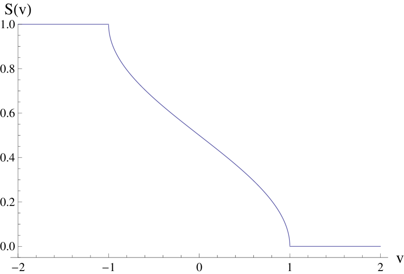
Figure 1: The density profile at late times $t$ converges to a scaling function $n_{m}(t)\to S\left(\frac{m}{t}\right)$. The figure shows a plot of $S(v)$ vs. $v$.

We now consider switching on the reset mechanism with rate $r$, discussed in the previous section. This resetting protocol will drive the density to a nontrivial stationary state. To see this, we compute the average density profile $n_{m}(r)$ of this fermionic chain in presence of a finite reset rate $r$. The calculation is quite easy and straightforward, given the general formalism in the previous section. We start from the expression of the stationary density matrix operator $\rho_{\rm stat}$ given in Eq. (10). The average stationary density profile, upon choosing the resetting time distribution $p(\tau|t)$ as in Eq. (7) with $t\to\infty$ is then given by

$$n_{m}(r) = \langle m|\rho_{\rm stat}|m\rangle=r\int_{0}^{\infty}d\tau\,e^{-r\tau}\,n_{m}(\tau)$$ (25)

where $n_{m}(\tau)$ is the average density profile at time $\tau$ without reset, and is given explicitly in Eqs. (20) and (21). Using this, we obtain, for $m>0$,

$$n_{m}(r)=\sum_{k=m}^{\infty}C_{k}(r)$$ (26)

where $C_{k}(r)=r\,\int_{0}^{\infty}J_{k}^{2}(\tau)\,e^{-r\tau}\,d\tau$. For $m\leq 0$, we have

$$n_{1-m}(r)=1-n_{m}(r)$$ (27)

which simply follows from Eq. (25) and the relation in Eq. (21). The function $C_{k}(r)$ can be explicitly expressed as

$$C_{k}(r) = \frac{4^{m}}{\pi}\Gamma^{2}(k+1/2)r^{-(2k)}$$ (28)

$$\times_{2}F_{1}(\frac{1}{2}+k,\frac{1}{2}+k,1+2k;-\frac{4}{r^{2}})$$

where $\Gamma$ denotes the Gamma function and ${}_{2}F_{1}$ is the regularized hypergeometric function. To get a feeling how the spatial density profile looks, we provide, in Fig. 2, a color plot of $n_{m}(r)$ as a function of $m$ and $r$ in the $(m-r)$ plane. The figure shows an exponential decay of $n_{m}(r)$ for large $m$, as well as for large $r$. We note that for large $r$, $n_{m}(r)\to 0$ for all $m$ which is the Zeno result showing that $n_{m}\to n_{m}(t=0)=\theta(-m)$ in this limit. For $r\to 0$, $n_{m}(r)$ approaches the value $n_{m}(t)$ at large $t$ (without reset), namely $n_{m}(r)\to 1/2$.

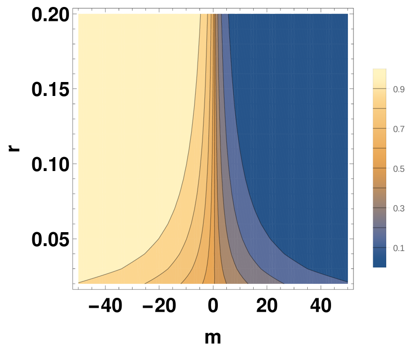
Figure 2: Plot of $n_{m}(r)$ as a function of $r$ and $m$ in the $(m-r)$ plane, showing exponential decay of $n_{m}(r)$ for large $m$ and large $r$.

Obtaining precisely the large $m$ asymptotic behavior of $n_{m}(r)$, for any fixed $r$, from the exact summation formula in Eqs. (26) and (28) turns out to be rather cumbersome. However, in the limit of small $r$, the large $m$ behavior can be derived precisely as follows. For small $r$, the integral in Eq. (25) is dominated by the large $t$ behavior of $n_{m}(t)$. Now, for large $m$ and large $t$, we can replace $n_{m}(t)$ by its scaling form, $n_{m}(t)=S(m/t)$, where $S(v)$ is given in Eq. (23). This gives, for large $m$ and $r\to 0$ (but fixed)

$$n_{m}(r)\approx\frac{r}{\pi}\int_{m}^{\infty}d\tau\,e^{-r\tau}\,\cos^{-1}\left(\frac{m}{\tau}\right)\,.$$ (29)

An integration by parts yields

$$n_{m}(r)=\frac{m}{\pi}\int_{m}^{\infty}d\tau\,\frac{e^{-r\tau}}{\tau\sqrt{\tau^{2}-m^{2}}}\,.$$ (30)

Next, we shift $\tau=m+x$, expand the integrand for large $m$ and carry out the integration over the first few terms of the expansion. This yields

$$n_{m}(r)\simeq\frac{e^{-rm}}{\sqrt{2\pi rm}}\,\left[1-\frac{5}{8}\,\frac{1}{rm}+\frac{128}{129}\,\frac{1}{(rm)^{2}}+\cdots\right]\,.$$ (31)

Thus the leading behavior of the steady state density profile at large $m$ is $n_{m}(r)\simeq e^{-mr}/\sqrt{2\pi rm}$. This agrees well with the exponential decay observed in numerics for large $m$ as long as $mr>1$, as can be seen in Fig. 3. Note that the steady state is parametrized by the value of reset rate $r$.

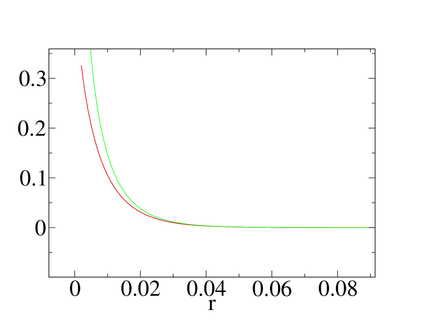
Figure 3: A comparison of plot of $n_{m}(r)$ as a function of $r$ with the analytic scaling form at large $m=100$.

The asymptotic result in Eq. (31) for large $m$ and fixed small $r$ suggests that there is a scaling limit $r\to 0$, $m\to\infty$, but with the product $x=rm$ fixed such that the density profile has a scale invariant form

$$n_{m}(r)\to F(r\,m)\,.$$ (32)

Indeed, we find that this is the case with the full scaling function $F(x)$ for all $x$, given explicitly by

$$F(x)=\frac{1}{\pi}\,\int_{x}^{\infty}K_{0}(|y|)\,dy\,.$$ (33)

where $K_{0}(y)$ is the modified Bessel function of index $0$. A derivation of this result in given in Appendix B. Note that $F(x)$ satisfies the symmetry relation,

$$F(-x)=1-F(x)\,.$$ (34)

A plot of this function is given in Fig. 4. Using the known asymptotics of $K_{0}(y)$, one can easily show that as $x\to\infty$

$$F(x)\to\frac{e^{-x}}{\sqrt{2\pi x}}\,\left[1-\frac{5}{8}\frac{1}{x}+\frac{128}{129}\frac{1}{x^{2}}+\cdots\right]\,,$$ (35)

in full agreement with the tail in Eq. (31). When $x\to-\infty$, one can use the symmetry relation in Eq. 34 and Eq. (35) to obtain the asymptotics. Clearly $F(x)\to 1$ as $x\to-\infty$. Furthermore, when $x\to 0$, we get

$$F(0)=\frac{1}{\pi}\int_{0}^{\infty}K_{0}(y)\,dy=\frac{1}{2}\,.$$ (36)

This is also consistent with the fact that $n_{m}(r)\to 1/2$ as $r\to 0$ (where $1/2$ is the average uniform density attained in the system at long times in the absence of reset).

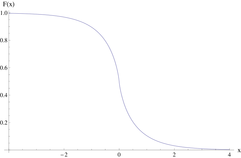
Figure 4: The scaling function $F(x)$ vs. $x$ in Eq. (33). It satisfies the symmetry property: $F(x)=1-F(-x)$.

III.2 Dirac Fermions

In this subsection, we shall study a class of periodically driven integrable models whose Hamiltonian can be represented by free Dirac fermions in $d$-dimensions:

$$H(t)=\sum_{\vec{k}}\psi_{\vec{k}}^{\dagger}H_{\vec{k}}(t)\psi_{\vec{k}},$$ (37)

where $\vec{k}$ is the $d$-dimensional momentum, $\psi_{\vec{k}}=(c_{\vec{k}},c_{-\vec{k}}^{\dagger})^{T}$ is the two-component fermionic field, $c_{\vec{k}}$ are the annihilation operators for the fermions, and $H_{\vec{k}}(t)$ is given by

$$H_{\vec{k}}=(g(t)-b_{\vec{k}})\tau^{z}+(\Delta_{\vec{k}}\tau^{+}+\rm{H.c.}).$$ (38)

Here $g(t)$ is a periodic function of time characterized by a time period $T$, and $\Delta_{\vec{k}}$ and $b_{\vec{k}}$ can be arbitrary functions of momenta whose specific forms depend on the particular physical system which the model (Eq. 37) represents. We note here that Eq. (37) may represent several integrable models such as the Ising and $XY$ models in $d=1$ [subirbook1, ], the Kitaev model in $d=2$ [kit1, ], triplet and singlet superconductors in $d>1$, and Dirac fermions in graphene and atop topological insulator surfaces [netorev, ; topoinrev, ]. In what follows, we shall first obtain general results by analyzing fermionic systems given by Eq. (38). The relevance of these results in the context of specific models will be discussed later in the section.

To study the dynamics of these periodically driven integrable models with resets, we choose the following protocol. We draw a random integer, $n$, from a distribution $P_{r}(n)$ of our choice characterized by the reset rate $r$ and let the system evolve for $n$ drive cycles starting from an initial state $|\psi_{0}\rangle$. After this, we measure correlation functions of the system. This is followed by a reset to the initial state $|\psi_{0}\rangle$. This process is repeated for several times and correlation functions are averaged over all measurements. The specific correlation functions used in our study shall be discussed in details later in this section.

To analyze the behavior of the correlation function in such dynamics, we first note that since these models are Gaussian, we would need to study only the quadratic fermionic correlators. The states of the system at $t=0$ and for any given $\vec{k}$ is given by

$$|\psi_{\vec{k}}\rangle=\left(\begin{array}[]{c}u_{\vec{k}}\\ v_{\vec{k}}\end{array}\right),\quad|\psi\rangle=\prod_{\vec{k}>0}|\psi_{\vec{k}}\rangle$$ (41)

where $u_{\vec{k}}[v_{\vec{k}}]=(1-[+](g(0)-b_{\vec{k}})/E_{\vec{k}})^{1/2}/\sqrt{2}$, and $E_{\vec{k}}=\sqrt{(g(0)-b_{\vec{k}})^{2}+\Delta_{\vec{k}}^{2}}$. For simplicity we shall start from an initial state $(u_{\vec{k}},v_{\vec{k}})=(0,1)$ and drive the system according to some periodic protocol with time period $T$ for $n$ periods. The quadratic fermionic correlators of the model are given by

$$C_{\vec{k}}(nT) = \langle\psi_{\vec{k}}(nT)|c_{\vec{k}}^{\dagger}c_{\vec{k}}|\psi_{\vec{k}}(nT)\rangle=|v_{n\vec{k}}|^{2}$$ (42)

$$F_{\vec{k}}(nT) = \langle\psi_{\vec{k}}(nT)|c_{\vec{k}}c_{-\vec{k}}|\psi_{)}{\vec{k}}(nT)\rangle=v^{*}_{n\vec{k}}(t)u_{n\vec{k}}$$

where $|\psi_{\vec{k}}(nT)\rangle=(u_{n\vec{k}},v_{n\vec{k}})^{T}$ is the wavefucntion of the system at momentum $\vec{k}$ and after $n$ drive cycles.

Next we note that for any periodic drive, the time periodicity of the Hamiltonian ensures that the unitary evolution operator at the end a drive cycle can be written as $U(0,T)=\exp[-iH_{F}T]$ where $H_{F}$ is the Floquet Hamiltonian [floquetrev1, ]. Consequently, the correlation functions of such driven systems, at the end of $n$ drive periods, can also be expressed in terms of eigenfunctions and eigenvectors of $H_{F}$ [floquetrev1, ; asen1, ]. For the class of integrable models that we treat here, one can show [asen1, ]

$$U_{\vec{k}} = \left(\begin{array}[]{cc}\cos(\theta_{\vec{k}})e^{i\alpha_{\vec{k}}}&\sin(\theta_{\vec{k}})e^{i\gamma_{\vec{k}}}\\ -\sin(\theta_{\vec{k}})e^{-i\gamma_{\vec{k}}}&\cos(\theta_{\vec{k}})e^{-i\alpha_{\vec{k}}}\\ \end{array}\right)=e^{-iH_{\vec{k}F}T}$$ (45)

where the parameters $\theta$, $\alpha$ and $\gamma$ can be found in terms of initial [$(u_{0},v_{0})=(0,1)$] and final [$(u_{\vec{k}},v_{\vec{k}})$] wavefunctions after one drive cycle as

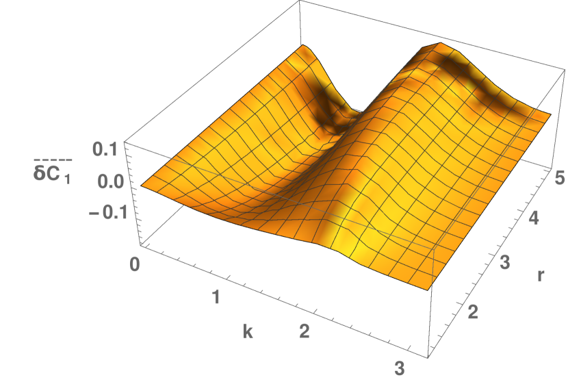
Figure 5: Plot of $\overline{\delta C_{1}}$ as a function of $k$ and $r$ for the pulse protocol with $g_{0}=2$, $g_{1}=0.5$ and $T=1$. All energies are scaled in units of $J$.

$$\sin(\theta_{\vec{k}}) = |u_{\vec{k}}|,\quad\alpha_{\vec{k}}(\gamma_{\vec{k}})={\rm Arg}[u_{\vec{k}}(v_{\vec{k}})]$$ (47)

For more general choice of the initial wavefunctions, the expressions for $\theta$, $\alpha$ and $\gamma$ can be found in Ref. asen1, . Furthermore, since $U_{\vec{k}}$ is a SU(2) matrix, one gets [asen1, ]

$$U_{\vec{k}} = e^{-i(\vec{\sigma}\cdot\vec{n}_{\vec{k}})\phi_{\vec{k}}},\quad n_{\vec{k}}=\frac{\vec{\epsilon}_{\vec{k}}}{|\vec{\epsilon}_{F\vec{k}}|}\quad,\phi_{\vec{k}}=T|\vec{\epsilon}_{F\vec{k}}|$$ (48)

where

$$n_{\vec{k}1} = -\sin(\theta_{\vec{k}})\sin(\gamma_{\vec{k}})\sin(\phi_{\vec{k}})/D_{\vec{k}}$$

$$n_{\vec{k}2} = -\sin(\theta_{\vec{k}})\cos(\gamma_{\vec{k}})\sin(\phi_{\vec{k}})/D_{\vec{k}}$$

$$n_{\vec{k}3} = -\cos(\theta_{\vec{k}})\sin(\alpha_{\vec{k}})\sin(\phi_{\vec{k}})/D_{\vec{k}}$$

$$D_{\vec{k}} = \sqrt{1-\cos^{2}(\theta_{\vec{k}})\cos^{2}(\alpha_{\vec{k}})}$$

$$|\vec{\epsilon}_{F\vec{k}}| = \arccos[\cos(\theta_{\vec{k}})\cos(\alpha_{\vec{k}})]/T.$$ (49)

Here ${\rm Sgn}$ denotes the signum function. Note that at the edge of the Brillouin zone, where the off-diagonal component of $H_{k}$ disappears, $U_{k}$ becomes a diagonal matrix, which in turns makes $\sin(\theta_{\vec{k}})=0$. This leads us to the result $n_{\vec{k}1}=n_{\vec{k}2}=0$ and $n_{\vec{k}3}=\pm 1$ for such momentum values.

Using the fact $|\psi_{\vec{k}}(nT)\rangle=U^{n}_{\vec{k}}|\psi_{\vec{k}}(0)$ and Eqs. (42..49), after some algebra, we can write

$$\delta C_{\vec{k}}(n) = f_{1}(\vec{k})\cos(2n\phi_{\vec{k}})$$ (50)

$$\delta F_{\vec{k}}(n) = (f_{2}(\vec{k})\cos(2n\phi_{\vec{k}})+f_{3}(\vec{k})\sin(2n\phi_{\vec{k}}))$$

where $\delta C_{\vec{k}}(n)=\langle c_{\vec{k}}^{\dagger}c_{\vec{k}}\rangle_{n}-\langle c_{\vec{k}}^{\dagger}c_{\vec{k}}\rangle_{\infty}$ and similarly for $\delta F_{\vec{k}}(n)$. In Eq. (50), the quantities $f_{1}(\vec{k})$, $f_{2}(\vec{k})$, and $f_{3}(\vec{k})$ are given in terms of elements of the Floquet Hamiltonian $H_{F}$ as

$$f_{1}(\vec{k}) = -(1-n^{2}_{\vec{k}3}),\quad f_{2}(\vec{k})=-i\hat{n}_{\vec{k}3}f_{3}(\vec{k})$$

$$f_{3}(\vec{k}) = i({n}_{\vec{k}1}+i{n}_{\vec{k}2}).$$ (51)

Note that $\delta C$ and $\delta F$ vanishes by construction for $n\to\infty$. The contribution to these terms comes from the off-diagonal terms of the density matrix in the Floquet basis as is evident from the presence of $\cos(2n\phi_{\vec{k}})$ and $\sin(2n\phi_{\vec{k}})$ factors in their expression [asen1, ]. For $n\to\infty$, the system is described by a generalized Gibbs ensemble (GGE) which is characterized by the values of the correlations $C_{\infty}(\vec{k})=1-n_{\vec{k}3}^{2}$ and $F_{\infty}(\vec{k})=-n_{\vec{k}3}(n_{\vec{k}1}+in_{\vec{k}2})$. Any deviation of the value of the fermionic correlators from $C_{\infty}$ or $F_{\infty}$ in the steady state therefore constitutes a different GGE representing that state. For this to happen, one clearly needs non-zero values of $\delta C$ or $\delta F$ for such steady states.

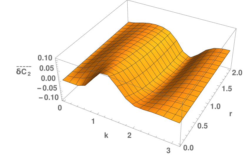
Figure 6: Plot of $\overline{\delta C}_{2}$ as a function of $k$ and $r$. All parameters are same as in Fig. 5.

Next, we look into the evolution of such a periodically driven model in the presence of resets characterized by $P_{r}(n)$ as discussed earlier. We note here that the resets do not mix the different $\vec{k}$ modes and hence retain the underlying integrability of the model. Thus we do not expect the steady-state density matrix to be given by a Gibbs ensemble with a characteristics temperature. The average value of $\delta C_{\vec{k}}$ and $\delta F_{\vec{k}}$, under such a reset protocol, is given by

$$\overline{\delta C_{\vec{k}}}(r)=\sum_{n=1}^{\infty}\delta C_{\vec{k}}(n)P_{r}(n)$$

$$\overline{\delta F_{\vec{k}}}(r)=\sum_{n=1}^{\infty}\delta F_{\vec{k}}(n)P_{r}(n)$$ (52)

Note that a finite value of ${\overline{\delta}C_{\vec{k}}}(r)$ or ${\overline{\delta}F_{\vec{k}}}(r)$ for any $k$ signifies a GGE characterized by $r$ which is different from the one at $r=0$. In what follows we shall focus on $\delta C$.

Below, we choose two different probability distributions for $P_{r}(n)$. The first one is given by $P_{r}(n)=[{\rm Li}_{r}(1)]^{-1}1/n^{r}$ for $r>1$ and $r\in Z$, where ${\rm Li}_{r}[1]=\sum_{n}(1/n^{r})$ is the PolyLog function. In the first case one obtains

$$\overline{\delta C_{1\vec{k}}}(r) = f_{1}(\vec{k}){\rm Re}[{\rm Li}_{r}(e^{2i\epsilon_{F\vec{k}}T})]/{\rm Li}_{r}[1]$$ (53)

where $\epsilon_{F\vec{k}}$ is the Floquet energy spectrum (Eq. 49).

The second one is the more well-known Poisson distribution for which $P_{r}(n)=r^{n}\exp[-r]/n!$. For this, we find

$$\overline{\delta C_{2\vec{k}}}(r) = f_{1}(\vec{k})[e^{-r(1-\cos(2\epsilon_{F\vec{k}}T))}$$ (54)

$$\times\cos[\sin(2\epsilon_{F\vec{k}}T)]-e^{-r}]$$

To check if $\overline{\delta C_{1}}$ (Eq. 53) and $\overline{\delta C_{2}}$ (Eq. 54) are finite functions of $r$ and $k$, we consider one-dimensional Ising model in a transverse field. The Hamiltonian of this model can be mapped to Eq. (37) with $b_{k}/J=\cos(k)$ and $\Delta_{k}/J=\sin(k)$, where $J$ is the interaction strength between neighboring Ising spins and $g=h/J$ is the strength of the transverse field. We plot $\overline{\delta C_{1}}$ and $\overline{\delta C_{2}}$ as a function of $k$ and $r$. We choose a periodic delta function pulse protocol $g(t)=g_{0}+g_{1}\sum_{n}\delta(t-nT)$ with $g_{0}=2$, $g_{1}=0.5$ and $T=1$. For this protocol, $\epsilon_{F\vec{k}}=\arccos[\cos(E_{\vec{k}}T)+(1-n_{3\vec{k}}^{2})\sin(E_{\vec{k}}T)]/T$ [asen1, ]. Substituting this in Eqs. (53), and (54), one may obtain $\delta C_{1(2)\vec{k}}$ as a function of $g_{0}$, $g_{1}$, $T$, $r$ and $\vec{k}$. The results, shown in Fig. 5 for $1/n^{r}$ distribution and Fig. 6 for the Poisson distribution, clearly indicates that both $\overline{\delta C_{1}}$ and $\overline{\delta C_{2}}$ are finite and functions of $r$ for all $k\neq 0,\pi$ where these correlations are identically zero (since $f_{1,2}=0$ and $f_{3}=1$ for these momenta). This clearly shows that stochastic resets lead to distinct family of GGEs characterized by a reset rate $r$ for periodically driven integrable quantum systems.

IV Bose-Hubbard model in a tilted optical lattice

In this section, we consider the stochastic dynamics of a Bose Hubbard model in the presence of a tilt, or an effective electric field. To see how such an electric field can be realized, first let us consider a typical Bose Hubbard model in a deep one-dimensional (1D) optical lattice (with lattice spacing $a$) so that the bosons are localized with $n=n_{0}$ bosons occupying each lattice site. The boson system is described by the well-known Bose-Hubbard Hamiltonian given by

$$H = -J\sum_{\langle rr^{\prime}\rangle}(b_{r}^{\dagger}b_{r^{\prime}}+{\rm h.c.})$$ (55)

$$+\sum_{r}(-\mu n_{r}+Un_{r}(n_{r}-1)/2)$$

where $J$ is the nearest neighbor hopping amplitude of the bosons, $U$ is the on-site interaction potential, and $\mu$ is the chemical potential. Here $b_{r}$ denotes the boson annihilation operator at site $r$, $n_{r}=b_{r}^{\dagger}b_{r}$ is the boson number operator, and $\langle..\rangle$ denotes sum over nearest neighboring sites of the lattice. We choose $J/U\ll 1$ and $\mu=\mu_{0}$ so that the ground state of $H$ represent a Mott localized state of bosons with $n_{0}$ bosons per site.

To generate a tilt for the bosons, the most experimentally convenient way is to apply a Zeeman magnetic field with varies linearly in space: $B(r)=B_{0}(r/a)$. The Zeeman term for this bosons can be written as $H_{z}=-\sum_{r}g\mu_{B}B_{0}(r/a)n_{r}=\sum_{r}{\mathcal{E}}rn_{r}$, where ${\mathcal{E}}=g\mu_{B}B_{0}/a$ is the effective electric field seen by the bosons, $B_{0}$ is the field amplitude, and $\mu_{B}$ is the Bohr magneton. The Hamiltonian of the system in the presence of the tilt is given by

$$H = -J\sum_{\langle rr^{\prime}\rangle}(b_{r}^{\dagger}b_{r^{\prime}}+{\rm h.c.})$$ (56)

$$+\sum_{r}(-(\mu+{\mathcal{E}}r)n_{r}+Un_{r}(n_{r}-1)/2)$$

The equilibrium and non-equilibrium properties of this Hamiltonian has been studied in several situations [subir1, ; dynamicsdipole, ]. To understand the property of such a system, it is first useful to note that a system of non-interacting bosons ($U=0$) in the presence of a tilted optical lattice constitutes a Wannier-Stark problem with exponentially localized wavefunctions. Thus, contrary to the classical expectation, bosons do not move to the last site to minimize their energy. Such a movement which constitutes an electric breakdown involves tunneling of the bosons to higher single particle bands. The time required for such breakdown for ultracold boson systems turns out to be larger than the system lifetime. Thus the parent boson state is preserved within experimental timescales. This feature is preserved, albeit with some difference, in the Mott regime where $U$ is large. The strategy for a theory of such a system thus involves identifying the low energy subspace around the parent Mott state which, in the presence of the electric field, is a metastable state with a very long lifetime [subir1, ].

It turns out that the low-energy theory of such a state can be formulated in terms of dipoles [subir1, ]. The creation of a dipole involves hopping of a boson from a site of the 1D lattice to its next neighbor. This costs an energy $U-{\mathcal{E}}$. Thus in the parameter regime where $U-{\mathcal{E}},J\ll U,{\mathcal{E}}$, the low-energy effective Hamiltonian of the bosons in a tilted lattice can be described in terms of dipole operators $d^{\dagger}_{\ell}=b_{j}^{\dagger}b_{i}/\sqrt{n_{0}(n_{0}+1)}$, where $\ell$ denotes the link between sites $i$ and $j$, as

$$H_{d} = -w\sum_{\ell}(d_{\ell}+d_{\ell}^{\dagger})+(U-{\mathcal{E}})\sum_{\ell}n_{\ell}.$$ (57)

Here $n_{\ell}=d_{\ell}^{\dagger}d_{\ell}$ is the dipole number operator and $w=J\sqrt{n_{0}(n_{0}+1)}$. The dipole model, so constructed, has two constraints. First, there can not be more than one dipole in a given site ($n_{\ell}\leq 1$) and second, there can not be two dipoles on adjacent links ($n_{\ell}n_{\ell+1}=0$) [subir1, ]. These constrains arise as the states which do not obey them can be shown not to be a part of the low-energy subspace with respect to the parent Mott state. It has been shown that the dipole model leads to two distinct ground states. The first is the dipole vacuum which occurs at $U>{\mathcal{E}}$; in the boson language this corresponds to the parent Mott state with $n_{0}$ bosons per sites. The second is the maximal dipole ground state occurring at ${\mathcal{E}}\geq{\mathcal{E}}_{c}=U+1.31w$ which corresponds to a $Z_{2}$ symmetry broken state with a dipole on odd or even links (but not both due to the second constraint mentioned above). In terms of the original boson model this state corresponds to $n_{0}+1$ and $n_{0}-1$ bosons on every alternate site. These two states are separated by a quantum phase transition belonging to the Ising universality class at ${\mathcal{E}}={\mathcal{E}_{c}}$. The quantum dynamics of the model by sudden, ramp and periodic time variation of the electric field has been studied in Ref. dynamicsdipole, .

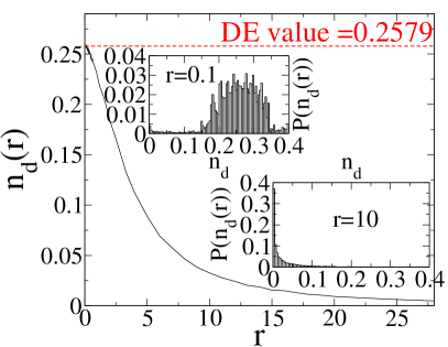
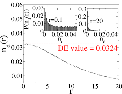
Figure 7: Plot of the dipole density $n_{d}(r)$ as a function of $r$ for (a) $U=E$ and (b) $(U-E)/w=-10$. The inset shows the probability distribution of $n_{d}$ at fixed $r$. The plots correspond to $N_{0}=10000$ and $N=12$.

Below, we compute the steady state expectation value of the dipole density operator $n_{d}=\sum_{\ell}n_{\ell}/N$, where $N$ is the number of lattice sites in the chain and we have set the lattice spacing to unity. We start from a dipole vacuum state which is the ground state of the system for $U>{\mathcal{E}}$ and $w=0$ and study its evolution under the dipole Hamiltonian $H_{d}$ with $(U-{\mathcal{E}}_{f})/w=0$ and $(U-{\mathcal{E}}_{f})/w=-10$ using exact diagonalization (ED). The former parameter corresponds to the system being near the critical point while the latter corresponds a maximal dipole ground state. The initial state of the system is denoted by $|\psi_{0}\rangle$ for which $\langle n_{d}\rangle=0$. The state of the system can be expressed at any instant $t>0$ as

$$|\psi(t)\rangle = \sum_{\alpha}c_{\alpha}e^{-i\epsilon_{\alpha}t}|m\rangle$$

$$H[{\mathcal{E}}_{f}]|\alpha\rangle = \epsilon_{\alpha}|\alpha\rangle\quad c_{m}=\langle m|\psi_{0}\rangle$$ (58)

where $\epsilon_{\alpha}$ and $|\alpha\rangle$ can be obtained numerical diagonalization of $H[{\mathcal{E}}_{f}]$. We note that since $H_{d}$ can be represented by a real symmetric matrix, $c_{\alpha}$ can be chosen to be real. We shall use this choice for the rest of the section. Using Eq. (58), one obtains

$$n_{d}(t) = \frac{1}{N}\sum_{\alpha\beta}c_{\alpha}c_{\beta}e^{-i\omega_{\beta\alpha}t}\langle\alpha|\sum_{\ell}n_{\ell}|\beta\rangle,$$ (59)

where $\omega_{\beta\alpha}=(\epsilon_{\beta}-\epsilon_{\alpha})$. Note that $n_{d}(t=0)=0$ since the initial state corresponds to a dipole vacuum. In contrast, the steady state (diagonal ensemble) value is finite and is found numerically to be $n_{d}(t\to\infty)=n_{d}^{\rm de}=0.2575$ for $U={\mathcal{E}}$. The corresponding value for $(U-{\mathcal{E}})/w=-10$ is $n_{d}^{\rm de}=0.0324$. The reason for a smaller value of $n_{d}^{\rm de}$ in the ordered phase can be understood as follows [dynamicsdipole, ]. First, we note that deep in the ordered phase $|\psi_{0}\rangle$ has substantial overlap with only a few of the eigenstates of the Hamiltonian; these eigenstates corresponds to $\langle n_{d}\rangle\simeq 0$. Thus $n_{d}^{\rm de}\simeq\sum_{\alpha}c_{\alpha}^{2}\langle\alpha|\hat{n}_{d}|\alpha\rangle$ remains small. In contrast, near the critical point, $|\psi_{0}\rangle$ has finite overlap with several eigenstates of the near-critical Hamiltonian leading to a larger value of $n_{d}^{\rm de}$.

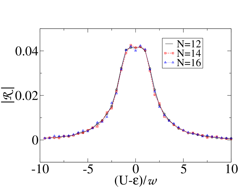
Figure 8: Plot of ${\mathcal{R}}$ as a function of $(U-{\mathcal{E}})/w$ for $N=12,\,14$, and $16$.

Next, we modify the unitary evolution following the quench with stochastic reset of the system at a time $\tau$ which is a random number with $P_{r}(\tau)=r\exp[-r\tau]$. Our numerical strategy for finding the effect of the reset is the following. First, we let the system evolve up to a time $\tau$ which is obtained using a random number generator and measure $n_{d}(\tau_{j}|t_{0})\equiv n_{d}(\tau_{j})$ at a fixed large $t_{0}$. We repeat this process for $N_{0}=10000$ and obtained average $n_{d}(r)=\sum_{j=1}^{N_{0}}P_{r}(\tau_{j})n_{d}(\tau_{j})$ from the data. Finally we repeat the procedure for several $r$. Note that since we can ignore the probability of having zero reset by formally choosing a large measurement time, the numerical procedure is expected to produce identical result to those obtained via Eqs. (10) and (16). We note that we have checked that for finite $r$, the system retains finite off-diagonal matrix elements of the density matrix for large $N_{0}$: $\langle m|\rho|n\rangle\neq 0$ for $m\neq n$ in the steady state. Thus the resultant deviation of $n_{d}$ or $S$ from their $r=0$ steady state values can not be interpreted as due to a steady state Gibb’s distribution with $r$ dependent temperature.

The results obtained from such a procedure are shown in Fig. 7(a) and 7(b) for $U={\mathcal{E}}$ and $(U-{\mathcal{E}})/w=-10$ respectively. We find that in both cases the steady state values of the dipole density with a fixed reset rate, $n_{d}(r)$, interpolates between $n_{d}(t=0)=0$ (for $r\to\infty$) and the diagonal ensemble value $n_{d}^{de}$ (for $r\to 0$). The $r$ dependence of $n_{d}(r)$ indicates that the steady state density matrix retains off-diagonal matrix elements and thus does not correspond to a diagonal density matrix for any finite $r$. We also note that the initial decrease of $n_{d}(r)$ from the diagonal ensemble value ($r=0$) to the Zeno (initial) value ($r\to\infty$) is faster for $U={\mathcal{E}}$. This feature can be qualitatively understood as follows. We note that the slope of $n_{d}(r)$ near $r=0$ can be expressed using Eq. (17) as

$${\mathcal{R}} = \frac{dn_{d}(r)}{dr}=\sum_{\alpha>\beta}c_{\alpha}c_{\beta}\langle\alpha|n_{d}|\beta\rangle\frac{2\omega_{\beta\alpha}^{2}r}{(r^{2}+\omega_{\beta\alpha}^{2})^{2}}.$$ (60)

where we have used the fact $\langle\alpha|n_{d}|\beta\rangle=\langle\beta|n_{d}|\alpha\rangle$. Note that near the critical point larger number of states have a finite overlap with $|\psi_{0}\rangle$ rendering a larger number $c_{\alpha}$s finite; this leads to enhancement of ${\mathcal{R}}$ for small but finite $r$. For $r=0$ and $r\to\infty$, the slope vanishes. A plot of $|{\mathcal{R}}(r=1)|$ for as a function of $(U-{\mathcal{E}})/w$ for a representative $r=1.2$ is shown in Fig. 8 confirming this expectation. Thus we find that $|{\mathcal{R}}|$ for a typical finite $r$ is sensitive to the presence of a critical point in the system and is expected to peak around it; however, its peak need not be at the precise location of the critical point.

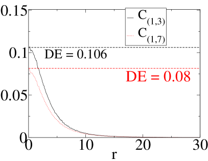
Figure 9: Left Panel: Plot of the dipole density-density correlation function $C_{\ell\ell^{\prime}}(r)$ for two representative values of $|\ell-\ell^{\prime}|$ as a function of $r$. Right Panel: Plot of the half chain entanglement $S(r)$ as a function of $r$. The inset shows $S(t)$ for a particular unitary time evolution between two resets after the quench. The diagonal ensemble state value of $S=2.18$ as can be seen from the inset. Both the plots correspond to $N_{0}=10000$, $U-{\mathcal{E}}/w=0$, and $N=12$.

Next we compute the dipole correlation function $C_{\ell,\ell^{\prime}}(r)=\langle\langle n_{d}(\ell)n_{d}(\ell^{\prime})\rangle\rangle$ where the expectations correspond to that with respect to $|\psi(\tau)\rangle$ and average over $P_{r}(\tau)$. The result is shown in Fig. 9(a) for $\ell=1$ and $\ell^{\prime}=3$ and $\ell^{\prime}=7$. The diagonal ensemble or the steady state value of this correlation function is shown via dotted horizontal lines in Fig. 9(a). Once again we find that the value of $C_{\ell\ell^{\prime}}(r)$ interpolates between its diagonal ensemble value for $r\to 0$ and the initial value for $r\to\infty$. In Fig. 9(b), we plot the half-chain entanglement

$$S(r) = \int_{0}^{\infty}dtre^{-rt}S(t),\,\,S(t)=-{\rm Tr}[\rho(t)\ln\rho(t)]$$

where the reduced density matrix $\rho$ for $N/2$ sites in the chain is computed numerically using ED. We note that $S(r)$ also interpolates between the diagonal ensemble $S(0)=S_{d}\simeq 2.52$ and the quantum Zeno (initial) $S(\infty)=S_{\rm initial}=0$ values. This confirms our expectation that the reset averaged steady state density matrix retains off-diagonal matrix elements.

Figure 10: Plot of $n_{d}(N_{0})$ as a function of the number of measurements $N_{0}$ showing $N_{0}$ independence of $n_{d}$ for large $N_{0}$. The plots correspond to $U-{\mathcal{E}}/w=0$, and $N=12$. See text for details.

Before ending this section, we show that the reset indeed leads to a steady state as discussed earlier. To this end, we plot the average value of the dipole density $n_{d}(N_{0})$ over $N_{0}$ measurements as a function of $N_{0}$ in Fig. 10 for several representative values of $r$. We find that $n_{d}(N_{0})$ indeed approaches a constant value as $N_{0}$ increases for any $r$ showing that the system reaches a steady state for large $N_{0}$. We have checked that a similar steady-state behavior is displayed by the correlation functions $C_{\ell\ell^{\prime}}$.

V Discussion

In this work, we have studied the unitary dynamics of quantum integrable and non-integrable systems interrupted by stochastic resets characterized by a rate $r$. For non-integrable models, such dynamics leads to a non-thermal steady state density matrix. Our analysis shows that such a dynamics leads to novel steady states for non-integrable and GGEs /statianory states for integrable quantum systems.

For non-integrable systems, we find that the density matrix, averaged over reset probability distribution, retains off-diagonal elements in the eigenbasis of the Hamiltonian controlling its unitary evolution. Thus such dynamics lead to non-diagonal steady state density matrices. This also indicates that the expectation value of a generic observable, averaged over the reset distribution, retain contribution from such off-diagonal terms. Thus the steady state value of the observable is no longer given by its average over a diagonal steady state density matrix as is customary for evolution without reset. We verify these results by explicit numerical calculation on Bose-Hubbard model on a tilted optical lattice which has been realized experimentally [greiner1, ]. We compute the dipole density, dipole density-density correlation and half-chain entanglement entropy of the model as a function of $r$. For all computed quantities, we find our results to agree with the diagonal ensemble result at $r=0$ and the quantum Zeno result for $r\to\infty$. In between, these quantities are smooth functions of $r$ indicating the finite contribution of the off-diagonal elements of the density matrix.

For integrable model, we have studied two separate examples. The first involves a spinless fermionic chain described by a hopping Hamiltonian with all the fermions occupying the left half of the chain. We study the behavior of the fermionic density $n_{m}(r)$ as a function of the reset rate and derive a scaling function which describes its stationary state behavior. Our results predicts a decay of the fermionic density as a function of the site index and reset rate as $n_{m}(r)\sim\exp[-mr]/\sqrt{2\pi mr}$ for $mr\gg 1$. The second example involves periodically driven Dirac fermions in the presence of resets. Here we have adapted a protocol where the system is allowed to evolve under a periodic drive for $n$ cycles where $n$ is a random integer chosen from a pre-determined distribution $P_{r}(n)$. After this evolution, the correlation functions of the system is computed and its state is reset to its initial value. This process is repeated and the average correlation is obtained summing over all measured values weighted by $P_{r}(n)$. This yields the steady state correlation function values for a finite $r$. We demonstrate that these values depend on $r$ indicating that the system is described by GGEs characterized by $r$.

Experimental verification of our results involves implementing the reset protocol. We note that such resets can be implemented by suitable projections of the quantum state to its initial value in ultracold atom systems by suitable laser pulses. For examples, such experiments have already been carried out leading to observation of the quantum Zeno effect. Such observations constituted experimental implementation of resets with $r\gg 1$ [mukund1, ]. We also note that finite chain of bosons in a tilted lattice have been experimentally realized [greiner1, ]. In such experiments, the dipole density computed in our work can be directly measured via parity of occupation measurement [greiner2, ; greiner1, ]. For experimental purpose, we would like to suggest measurement of bosonic dipole density as a function of $r$. For this, one would need to reset the system to the dipole vacuum state with a finite rate. This can in principle be done by changing the value of the electric field to a small value and letting the system equilibrate to the ground state of the resultant Hamiltonian [greiner1, ]. We predict that the reset averaged value of the dipole density would be a smooth decaying function of $r$ and would be qualitatively similar to that shown in Fig. 7.

To conclude, we have studied the dynamics of quantum systems in the presence of stochastic resets and have shown that the steady state density matrices, averaged over reset probability distribution, retains off-diagonal terms. We also show that such dynamics for integrable models leads to family of GGEs/stationary states characterized by a reset probability $r$. We have discussed experiments using ultracold bosons which can test our theory.

We note that after our work was completed, Ref. [garrahan1, ], which studies the spectral properties of quantum systems under random resets using a different approach, appeared on the arXiv.

Acknowledgments

S.N.M acknowledges support from ANR grant ANR-17-CE30-0027-01 RaMaTraF and the Indo-French Centre for the promotion of advanced research (IFCPAR) under Project No. 5604-2.

Appendix A Application to single particle quantum mechanics

In this appendix, we are going to chart out the effect of reset on two simple single particle quantum mechanical systems. The first constitutes the evolution of a Gaussian wavepacket under reset while the second involves that of a coherent state of a simple harmonic oscillator.

For the first case, we consider a 1D Gaussian wavepacket whose normalized wavefunction at $t=0$ is given by

$$\psi(x,0) = \exp[-x^{2}/(2\sigma^{2})]/\sqrt{2\pi\sigma}$$ (62)

$$= \frac{\sqrt{\sigma}}{2\pi}\int dke^{ikx}e^{-k^{2}\sigma^{2}/2}$$

where $\sigma$ quantifies the spread of the wavepacket in real space. For a free particle with $H=k^{2}/(2m)$, the wavefunction at any time $t$ is given by

$$\psi(x,t) = \frac{\sqrt{\sigma}}{\sqrt{2\pi(\sigma^{2}+it/m)}}e^{-\frac{x^{2}}{2(\sigma^{2}+it/m)}}$$ (63)

Note that this indicates a ballistic spread of the wavepacket as is customary in quantum mechanics. Now consider an evolution with reset characterized by the reset time distribution $p(\tau|t_{0})$ given in Eq. (7), with the measurement time $t_{0}\to\infty$. Then the stationary probability density, characterized by the square of the absolute value of wavefunction averaged over the reset time distribution, is given by

$$P(x;r) = \int_{0}^{\infty}d\tau re^{-r\tau}|\psi(x,\tau)|^{2}$$ (64)

For large $x$, the integral in Eq. (64) can be evaluated by saddle point method and yields $P(x;r)\simeq\exp[-c(|x|^{2}/r)^{1/3}]$, where $c$ is a constant independent of $r$. This stretched exponential behavior of the tail of the probability distribution is to be contrasted with its counterpart for a diffusive classical system for which $P\sim\exp[-c^{\prime}|x^{2}/r|^{1/2}]$ where $c^{\prime}$ is a constant [EM12011, ]. The difference in these two behaviors originates from the ballistic nature of the spread of the wavepacket in the quantum case.

For the second case, we consider a coherent state for a simple harmonic oscillator given by

$$|\alpha(t)\rangle = e^{-|\alpha|^{2}/2}\sum_{n}\frac{\alpha^{n}}{{\sqrt{n}!}}e^{-i\omega_{n}t}|n\rangle$$ (65)

where $\omega_{n}=E_{n}=\omega_{0}(n+1/2)$ denotes frequencies corresponding to harmonic oscillator energy levels, $\omega_{0}$ is the natural oscillator frequency.

Now consider a typical element of the density matrix constructed out of this coherent state wavefunction. This is given by

$$\rho_{mn}=e^{-|\alpha|^{2}}\frac{[\alpha^{n}(\alpha^{*})^{m}]}{\sqrt{m!n!}}e^{i(m-n)\omega_{0}t}$$ (66)

In the absence of any reset, the long time average of any off diagonal terms vanishes. This leads to the diagonal ensemble. However, if we now introduce Stochastic reset with $P(r)=re^{-rt}$ we find finite off-diagonal elements

$$\langle\rho_{mn}\rangle=e^{-|\alpha|^{2}}\frac{[\alpha^{n}(\alpha^{*})^{m}]}{\sqrt{m!n!}}\frac{r(r-i\omega_{0}(n-m))}{r^{2}+(n-m)^{2}\omega_{0}^{2}}$$ (67)

The presence of such finite off-diagonal elements is manifested in several physical quantities. For example, the mean position of the wavepacket, without reset, is given by (assuming real $\alpha$ without loss of generality) $X(t)=\sqrt{2/\omega_{0}}\alpha\cos(\omega_{0}t)$. Note that the time average of $X$ vanishes signifying localization of the wavepacket; thus the diagonal ensemble result corresponds to $X(t\to\infty)=0$. In contrast, the time average of $X$ with the reset is

$${\overline{X}}(r) = \int_{0}^{\infty}dtre^{-rt}X(t)=\sqrt{\frac{2\alpha^{2}}{\omega_{0}}}\frac{r^{2}}{r^{2}+\omega_{0}^{2}}$$ (68)

The result interpolates between Zeno ($r\to\infty$) and diagonal ensemble ($r\to 0$) limits as expected. This demonstrates that the mean position of the coherent state wavepacket can be controlled by the reset rate $r$.

Appendix B Derivation of the scaling function $F(x)$ in Eq. (33)

We start from the exact expression for $n_{m}(r)$ in Eq. (26), where

$$C_{k}(r)=r\int_{0}^{\infty}J_{k}^{2}(\tau)\,e^{-r\tau}\,d\tau\,.$$ (69)

Next we use the exact identity [martin2008, ]

$$\int_{0}^{\infty}J_{k}^{2}(t)\,e^{-r\tau}\,d\tau=\frac{1}{4\pi}\int_{-\pi}^{\pi}d\theta\,\frac{e^{ik\theta}}{\sqrt{\frac{r^{2}}{4}+\sin^{2}\left(\frac{\theta}{2}\right)}}\,.$$ (70)

Making the change of variable $k\theta=q$ gives

$$C_{k}(r)=\frac{r}{4\pi k}\,\int_{-k\pi}^{k\pi}dq\frac{e^{iq}}{\sqrt{\frac{r^{2}}{4}+\sin^{2}\left(\frac{q}{2k}\right)}}\,.$$ (71)

We now take the scaling limit, $r\to 0$, $k\to\infty$, while keeping the product $y=rk$ fixed. Setting $k=y/r$ with $y$ fixed we get

$$C_{k=y/r}(r)=\frac{r^{2}}{4\pi\,y}\,\int_{-\pi\,y/r}^{\pi\,y/r}dq\frac{e^{iq}}{\sqrt{\frac{r^{2}}{4}+\sin^{2}\left(\frac{qr}{2y}\right)}}\,.$$ (72)

In the limit $r\to 0$ (with fixed $y$), we can send the limits of integrations to $\pm\infty$ and also expand the sine in the denominator to leading order for small argument. This leads to

$$C_{k=y/r}(r)\approx\frac{r}{2\pi}\int_{-\infty}^{\infty}\frac{dq\,e^{iq}}{\sqrt{q^{2}+y^{2}}}\,.$$ (73)

The integral can be recognized as $2\,K_{0}(|y|)$. Hence, we get the result in the scaling limit

$$C_{k}(r)\approx\frac{r}{\pi}\,K_{0}(r|k|)\,.$$ (74)

Finally, from Eq. (26), we get in the scaling limit (where the sum in Eq. (26) can be replaced by an integral as $r\to 0$)

$$n_{m}(r)=\sum_{k=m}^{\infty}C_{k}(r) \approx \sum_{k=m}^{\infty}r\,K_{0}(r|k|)$$ (75)

$$\approx \frac{1}{\pi}\int_{rm}^{\infty}K_{0}(|y|)\,dy)$$

This gives the result in Eqs. (32) and (33).

References

- (1) J. Dziarmaga, Adv. Phys. 59, 1063 (2010).
- (2) A. Polkovnikov, K. Sengupta, A. Silva, and M. Vengalattore, Rev. Mod. Phys. 83, 863 (2011).
- (3) A. Dutta, U. Divakaran, D. Sen, B.K. Chakrabarti, T.F. Rosenbaum, G. Aeppli, arXiv:1012.0653 (unpublished); S. Mondal, D. Sen and K. Sengupta, Lect. Notes Phys. 21, 802 (2010).
- (4) I. Bloch, J. Dalibard, and W. Zwerger, Rev. Mod. Phys. 80, 885 (2008).
- (5) L. D’Alessio, Y. Kafri, A. Polkovnikov and M. Rigol, Adv. Phys. 65, 239 (2016).
- (6) K. Sengupta, S. Powell, and S. Sachdev, Phys. Rev. A69, 053616 (2004)
- (7) P. Calabrese and J. Cardy, Phys. Rev. Lett. 96, 136801 (2006); ibid, J. Stat. Mech. 0706 P06008 (2007).
- (8) T.W.B. Kibble, J. Phys. A: Math. Gen. 9, 1387 (1976); ibid, Phys. Rep. 67, 183 (1980)
- (9) W.H. Zurek, Nature (London) 317, 505 (1985); ibid Phys. Rep. 276, 177 (1996); B. Damski, Phys. Rev. Lett. 95, 035701 (2005); W.H. Zurek, U. Dorner, and P. Zoller, Phys. Rev. Lett. 95, 105701 (2005)
- (10) A. Polkovnikov, Phys. Rev. B 72, 161201(R) (2005); R. Barankov, A. Polkovnikov, Phys. Rev. Lett. 101, 076801 (2008); A. Chandran, A. Erez, S.S. Gubser, S.L. Sondhi, Phys. Rev. B 86, 064304 (2012).
- (11) K. Sengupta, S. Mondal, and D. Sen, Phys. Rev. Lett. 100, 077204 (2008); S. Mondal, D. Sen and K. Sengupta, Phys. Rev. B 78 (2008) 045101.
- (12) D. Sen, S. Mondal, K. Sengupta, Phys. Rev. Lett. 101, 016806 (2008);
- (13) J.D. Sau, K. Sengupta, Phys. Rev. B 90, 104306 (2014); U. Divakaran, K. Sengupta, Phys. Rev. B 90, 184303 (2014).
- (14) C. De Grandi and A. Polkovnikov, in Quantum Quenching, Annealing, and Computation, edited by A. K. Chandra, A. Das, and B. K. Chakrabarti, Lecture Notes in Physics, 802, 75 (Springer, Heidelberg, 2010).
- (15) S.R. Das, D.A. Galante and R.C. Myers, Phys. Rev. Lett. 112 171601 (2014); ibid, JHEP 02 167 (2015); D. Das, S. R. Das, D. A. Galante, R. C. Myers, and K. Sengupta, JHEP 11, 157 (2017).
- (16) M. Rigol, V. Dunjko and M. Olshanii, Nature 452 854 (2008).
- (17) J.M. Deutsch, Phys. Rev. A 43 2046 (1991).
- (18) M. Srednicki, Phys. Rev. E 50, 888 (1994); ibid J. Phys. A 32, 1163 (1999).
- (19) A. Lazarides, A. Das, and R. Moessner, Phys. Rev. Lett. 112, 150401 (2014); ibid, Phys. Rev. E 90, 012110 (2014); P. Ponte, A. Chandran, Z. Papic, and D. A. Abanin, Ann. Phys. (Amsterdam) 353, 196 (2014); L. D’Alessio and M. Rigol, Phys. Rev. X 4, 041048 (2014)
- (20) S. Nandy, A. Sen, and D. Sen, Phys. Rev. X 7, 031034 (2017).
- (21) M. R. Evans and S. N. Majumdar, Phys. Rev. Lett. 106, 160601 (2011).
- (22) M. R. Evans and S. N. Majumdar, J. Phys. A: Math. Theor. 44, 435001 (2011).
- (23) M. R. Evans and S. N. Majumdar, J. Phys. A: Math. Theor. 47, 455004 (2014).
- (24) S. Gupta, S. N. Majumdar, and G. Schehr, Phys. Rev. Lett. 112, 220601 (2014).
- (25) X. Durang, M. Henkel, and H. Park, J. Phys. A: Math. Theor. 47, 045002 (2014).
- (26) S. N. Majumdar, S. Sabhapandit, and G. Schehr, Phys. Rev. E 91, 052131 (2015).
- (27) S. N. Majumdar, S. Sabhapandit, and G. Schehr, Phys. Rev. E 92, 052126 (2015).
- (28) A. Pal, Phys. Rev. E 91, 012113 (2015).
- (29) S. Eule and J. J. Metzger, New J. Phys. 18, 033006 (2016).
- (30) A. Nagar and S. Gupta, Phys. Rev. E 93, 060102 (2016).
- (31) D. Boyer, M. R. Evans, and S. N. Majumdar, J. Stat. Mech. P023208 (2017).
- (32) A. Pal, A. Kundu, and M. R. Evans, J. Phys. A. Math. Theor. 49, 225001 (2016).
- (33) A. Falcon-Cortes, D. Boyer, L. Giuggioli, and S. N. Majumdar, Phys. Rev. Lett. 119, 140603 (2017).
- (34) C. Maes and T. Thiery, J. Phys. A. Math. Theor. 50, 415001 (2017).
- (35) E. Roldan and S. Gupta, Phys. Rev. E 96, 022130 (2017).
- (36) S. Redner, A Guide to First-Passage Processes, (Cambridge University Press, Cambridge, 2001).
- (37) A. J. Bray, S. N. Majumdar, and G. Schehr, Adv. in Phys. 62, 225 (2013).
- (38) M. R. Evans, S. N. Majumdar, and K. Mallick, J. Phys. A: Math. Theor. 46, 185001 (2013).
- (39) J. Whitehouse, M. R. Evans, and S. N. Majumdar, Phys. Rev. E 87, 022118 (2013).
- (40) M. Montero and J. Villarroel, Phys. Rev. E 87, 012116 (2013).
- (41) L. Kusmierz, S. N. Majumdar, S. Sabhapandit, and G. Schehr, Phys. Rev. Lett. 113, 220602 (2014).
- (42) S. Reuveni, M. Urbach, and J. Klafter, Proc. Natl. Acad. Sci. USA 111, 4391 (2014).
- (43) C. Christou and A. Schadschneider, J. Phys. A: Math. Theor. 48, 285003 (2015).
- (44) S. Reuveni, Phys. Rev. Lett. 116, 170601 (2016).
- (45) U. Bhat, C. De Bacco, and S. Redner, J. Stat. Mech. P083401 (2016).
- (46) M. Montero, M. Maso-Puigdellosas, and J. Villarroel, Eur. Phys. J. B 90, 176 (2017).
- (47) A. Pal and S. Reuveni, Phys. Rev. Lett. 18, 030603 (2017).
- (48) J. M. Meylahn, S. Sabhapandit, and H. Touchette, Phys. Rev. E 92, 062148 (2015)
- (49) R. J. Harris and H. Touchette, J. Phys. A: Math. Theor. 50, 10LT01 (2017).
- (50) F. den Hollander, S.N. Majumdar, J. M. Meylahn, and H. Touchette, arXiv: 1801.09909
- (51) J Fuchs, S Goldt, and U Seifert, EuroPhys. Lett. 113, 6 (2016).
- (52) A. Pal and S. Rahav, Phys. Rev. E 96, 062135 (2017).
- (53) T. Albash, D.A. Lidar, M. Marvian, and P. Zanardi, Phys. Rev. A 88, 023146 (2013); A.E. Rastegin, J. Stat. Mech. P06016 (2013); D. Kafri and S. Deffner, Phys. Rev. A 86, 044302 (2012); M. Campisi, J. Pekola, and R. Fazio, New J. Phys. 19, 053027 (2017); S. Gherardini, L. Buffoni, M. M. Muller,, F. Caruso, M. Campisi, A. Trombettoni, and S. Ruffo, arXiv:1805.00773 (unpublished).
- (54) S. Dhar, S. Dasgupta, A. Dhar, and D. Sen, Phys. Rev. A 91, 062115 (2015).
- (55) F. Thiel. E. Barkai, and D. A. Kessler, Phys. Rev. Lett. 120, 040502 (2018); H. Friedman, D. A. Kessler, and E. Barkai, Phys. Rev. E95, 032141 (2017).
- (56) C. B. Chiu, E. C. G. Sudershan, and B. Misra, Phys. Rev. D 16, 520 (1977); W. M. Itano, D. J. Heinzen, J. J. Bollinger, and D. J. Wineland Phys. Rev. A 41, 2295 (1990); D. Home and M. A. B Whittaker, Ann. Phys. 258, 237 (1997).
- (57) S. Sachdev, K. Sengupta, and S. M. Girvin, Phys. Rev. B66 075128 (2002); S. Pielawa, T. Kitagawa, E. Berg, and S. Sachdev, Phys. Rev. B 83, 205135 (2011); C. P. Rubbo, S. R. Manmana, B. M. Peden, M. J. Holland, and A. M. Rey, Phys. Rev. A 84, 033638 (2011).
- (58) W. S. Bakr, A. Peng, M. E. Tai, R. Ma, J. I. Gillen, and S. F ollen, Science 329, 547 (2010).
- (59) J. Simon, W. Bakr, R. Ma, M. E. Tai, P. Preiss, and M. Greiner, Nature (London) 472, 307 (2011).
- (60) T. Antal, Z. Racz, A. Rakos, and G. M. Schutz, Phys. Rev. E 59, 4912 (1999).
- (61) T. Antal, P. L. Krapivsky, and A. Rakos, Phys. Rev. E 78, 06115 (2008).
- (62) V. Eisler and Z. Racz, Phys. Rev. Lett. 110, 060602 (2013); V. Hunyadi, Z. Racz, and L. Sasvari, Phys. Rev. E69, 066103 (2004).
- (63) S. Sachdev, Quantum Phase Transitions, (Cambridge University Press, Cambridge, 1999).
- (64) A. Kitaev, Ann. Phys. (N.Y.) 321, 2 (2006).
- (65) A. H. Castro Neto, F. Guinea, N. M. R. Peres, K. S. Novoselov, and A. K. Geim, Rev. Mod. Phys. 81, 109 (2009).
- (66) M. Z. Hasan and C. L. Kane, Rev. Mod. Phys. 82, 3045 (2010).
- (67) A. Eckardt Rev. Mod. Phys. 89, 011004 (2017).
- (68) A. Sen, S. Nandy, and K. Sengupta, Phys. Rev. B94, 214301 (2016).
- (69) K. Sengupta, S. Powell, and S. Sachdev, Phys. Rev. A69, 053616 (2004); M. Kolodrubetz, D. Pekker, B. K. Clark, and K. Sengupta, Phys. Rev. B85, 100505(R) (2012); U. Divakaran and K. Sengupta, Phys. Rev. B90, 184303 (2014); R. Ghosh, A. Sen, and K. Sengupta, Phys. Rev. B97, 014309 (2018).
- (70) Y. S. Patil, S. Chakram, and M. Vengalattore, Phys. Rev. Lett. 115, 140402 (2015); Y. S. Patil, S. Chakram, L. M. Aycock, and M. Vengalattore, Phys. Rev. A90, 033422 (2014).
- (71) P. A. Martin, J. Phys. A. Math. Theor. 41, 015207 (2008).
- (72) D. C. Rose, H. Touchette, I. Lesanovsky, and J. P. Garrahan, arXiv:1806.01298 (unpublished).