Microscopic description of displacive coherent phonons

Abstract

We develop a Hamiltonian-based microscopic description of laser pump induced displacive coherent phonons. The theory captures the feedback of the phonon excitation upon the electronic fluid, which is missing in the state-of-the-art phenomenological formulation. We show that this feedback leads to chirping at short time scales, even if the phonon motion is harmonic. At long times this feedback appears as a finite phase in the oscillatory signal. We apply the theory to BaFe₂As₂, explain the origin of the phase in the oscillatory signal reported in recent experiments, and we predict that the system will exhibit red-shifted chirping at larger fluence. Our theory also opens the possibility to extract equilibrium information from coherent phonon dynamics.

I Introduction

The development of femtosecond laser pumps has led to new probes of complex metals whereby systems are driven out of equilibrium with the aim to study their relaxation dynamics [1; 2; 3]. Simultaneously, pump-probe setups allow the fascinating possibility to study phenomena that have no analog in equilibrium physics, such as the transient excitation of coherent optical phonons [4; 5; 6; 7]. A “coherent” phonon is excited when the relevant atoms of the crystalline solid, which are macroscopic in number, vibrate with identical frequency and phase [see Fig. 1(a)]. This is to be contrasted with incoherent motion triggered by quantum and thermal fluctuations in equilibrium where, from atom to atom, the frequencies and phases are uncorrelated. More recently it has been recognized that the physics of Floquet dynamics can be made experimentally accessible via coherent phonon excitations [8; 9].

Experimentally, a typical signature of a coherent phonon excitation is an oscillatory signal on a decaying background in time-resolved spectroscopic probes such as x-ray spectroscopy, photoemission and reflectivity measurements. Coherent phonons have been studied in a variety of materials that include semiconductors [10; 11; 12], semimetals [13; 14; 15; 16; 17; 18; 19], transition metals [20], Cu-based [21; 22; 23; 24] and the Fe-based [25; 26; 27; 28; 29; 30; 31; 32; 33] high temperature superconductors, charge density wave systems [34; 35; 36; 37; 38], as well as Mott [39; 40; 41; 42] and topological [43; 44; 45] insulators.

On the theory side, this phenomenon is usually described either as displacive excitaion of coherent phonons (DECP) [46; 47] or as impulsive stimulated Raman scattering (ISRS) [48; 49]. In the former mechanism photoexcitation leads to a shift in the equilibrium position of the phonon [46; 47], while in the latter the electromagnetic radiation provides a short impulsive force to the atoms [48; 49]. Note, if the photoexcitation does not involve crossing phase boundaries, then typically only the fully symmetric Raman $A_{1g}$ phonon is excited in DECP. It has been argued that in absorbing medium these two mechanisms are not distinct [50]. Using the above concepts, first-principles calculations have been successfully applied to understand coherent phonon dynamics in a variety of systems [51; 52; 53; 54; 55].

The purpose of this work is to develop, within the conceptual framework of DECP, a microscopic Hamiltonian-based description of coherent phonons in an environment where the timescale for the photoexcited carriers to thermalize is rather short, such as a metal with gapless charge excitations. Here we focus on coherent phonon excitation driven by laser heating of carriers, a phenomena which is relevant experimentally, but which has received less attention theoretically. As we show below, the microscopic formulation provides a better treatment of electron-phonon interaction compared to the phenomenological model that is currently used to analyze experimental data [46]. In particular, our theory captures how the coherent phonon excitation modifies the electronic fluid, and how this modification feeds back on the coherent phonon dynamics.

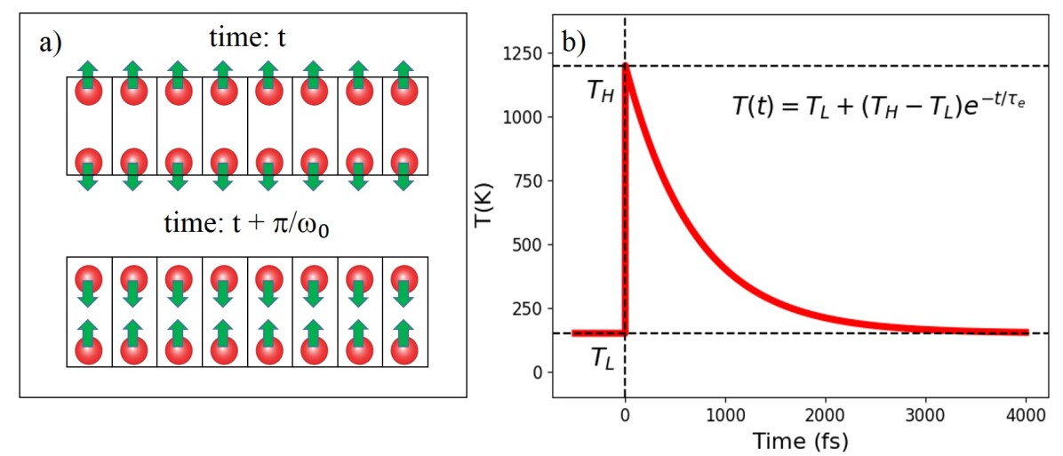
Figure 1: (color online) (a) Sketch of an $A_{1g}$ coherent phonon motion in a two-atom (red balls) unit cell. A macroscopic number of atoms oscillate with identical phase and frequency $\omega_{0}$. Green arrows indicate the instantaneous velocities at two instants. The motion preserves the point group symmetry. (b) The effect of the laser pump is idealized as a temperature quench from a measured base temperature $T_{L}$ to a high temperature $T_{H}$ over a short time set to zero, and the subsequent relaxation of temperature over a time-scale $\tau_{e}$. In the theory, $(T_{H},\tau_{e})$ are phenomenological parameters (see text). The temperature and time scales are representative.

The main advances of our work compared to the phenomenological theory of Zeiger ² [46] are the following. (i) Including the lattice feedback effect leads to a richer description of the dynamics. In particular, we show that at short time scales this leads to chirping or temporal variations of the oscillation frequency, while staying within a harmonic description of the coherent phonons. On the other hand, at long times the feedback leads to a finite phase in the oscillatory signal. The origin of this phase is distinct from that in the phenomenological DECP theory [46], and it is likely to be dominant quantitatively. Importantly, the theory predicts that the sign of the phase is determined by whether the chirping is red or blue shifted. (ii) A Hamiltonian formulation opens the possibility of extracting microscopic equilibrium information from coherent phonon studies. (iii) The microscopic formulation can be refined systematically using methods of many-body to deal with various interaction effects.

The paper is organized as follows. In Sec. II, we introduce the microscopic model, we discuss the rationale for treating the effect of the pump as a quench of the electronic temperature, and we derive the equation of motion of the coherent phonon using Heisenberg equation of motion. In Sec. III, we solve the above equation, and we discuss our main results, emphasizing the new physics introduced by taking into account the feedback of the lattice. In Sec. IV, we apply the theory to BaFe₂As₂ and we show that the data from a recent time resolved x-ray study can be successfully described by our theory, using a more constrained fit. We conclude in Sec. V.

II Model & Formalism

We consider a multiorbital electronic system interacting with a zero wavevector uniform $A_{1g}$ phonon mode. It is described by the Hamiltonian

$$\mathcal{H} =\sum_{{\bf k},a,b,\sigma}\left[\epsilon({\bf k})_{ab}-\mu\delta_{ab}\right]c^{\dagger}_{{\bf k}a\sigma}c_{{\bf k}b\sigma}+\mathcal{N}\hbar\omega_{0}(b^{\dagger}b+1/2)$$

$$+\lambda\sum_{{\bf k},a,b,\sigma}C({\bf k})_{ab}c^{\dagger}_{{\bf k}a\sigma}c_{{\bf k}b\sigma}(b^{\dagger}+b).$$ (1)

$\epsilon({\bf k})_{ab}$ describe the dispersion in an orbital basis, and $\mu$ is the chemical potential. $c^{\dagger}_{{\bf k}a\sigma}$ and $c_{{\bf k}a\sigma}$ are electron creation and annihilation operators, respectively, with lattice wavevector ${\bf k}$, orbital index $a$, and spin $\sigma$. The operators ($b^{\dagger}$, $b$) describe creation and annihilation operators for the $A_{1g}$ phonon with frequency $\omega_{0}$, and $\mathcal{N}$ is the total number of sites. Electron-phonon interaction is described by $\lambda C({\bf k})_{ab}$, where $\lambda<1$ is a dimensionless small parameter and $C(k)_{ab}$ is order Fermi energy. Thus, electron-phonon interaction can be treated perturbatively in orders of $\lambda$. For clarity, we ignore the phonon modes that are not coherently generated. We also ignore electron-electron and phonon-phonon interaction. Later, we comment on their effects.

After the pump the initial dynamics of the system is dominated by light-matter and by electron-electron interactions. However, as time and angle resolved photoemission (tr-ARPES) experiments have shown [19; 30], due to electron-electron scattering the electronic subsystem equilibrates after a time $\tau_{r}$ of order few tens of femtoseconds. At longer times an instantaneous electronic temperature $T(t)$ can be defined. In this work we focus on the regime $t\gg\tau_{r}$. Accordingly, we assume $\tau_{r}\rightarrow 0$, such that the effect of the laser pump can be modeled as inducing a temperature quench of the electrons. We assume that the electronic temperature relaxation is characterized by a timescale $\tau_{e}$, and is described phenomenologically by

$$T(t)=T_{L}+(T_{H}-T_{L})\operatorname{e}^{-t/\tau_{e}},$$ (2)

where $T_{L}\equiv T(t=0^{-})=T(t\rightarrow\infty)$, and $T_{H}\equiv T(t=0^{+})$ [see Fig. 1(b)].

The dimensionless mean atomic displacement $u\equiv\langle b+b^{\dagger}\rangle$ follows the equation of motion $\left(\partial_{t}^{2}+\omega_{0}^{2}\right)u=F(t)$, where the out-of-equilibrium force is

$$F(t)=-\frac{2\omega_{0}}{\mathcal{N}}\lambda\sum_{{\bf k},a,b,\sigma}C({\bf k})_{ab}\langle c^{\dagger}_{{\bf k}a\sigma}(t)c_{{\bf k}b\sigma}(t)\rangle_{\mathcal{H},T(t)}.$$

Here $\langle X\rangle_{\mathcal{H},T(t)}\equiv{\rm Tr}[\rho X]/{\rm Tr}[\rho]$ and $\rho\equiv|n\rangle\langle n|\operatorname{e}^{-E_{n}/T(t)}$, where $|n\rangle$ and $E_{n}$ are the eigenfunctions and eigenvalues, respectively, of $\mathcal{H}$ in Eq. (II).

Our goal is to capture, at least qualitatively, the feedback of the coherent phonon on the electron fluid, for which it is sufficient to evaluate the force to second order in $\lambda$. At this order $u(t)$ can be treated as a classical variable fluctuating in time, and $F(t)$ can be evaluated using linear response theory. We get

$$F(t)/(2\omega_{0})=-\langle\hat{O}\rangle_{\mathcal{H}_{0},T(t)}-\int_{-\infty}^{\infty}dt^{\prime}\Pi_{T(t)}(t-t^{\prime})u(t^{\prime}),$$ (3)

where $\Pi_{T(t)}(t-t^{\prime})\equiv i\theta(t-t^{\prime})\langle\left[\hat{O}(t^{\prime}),\hat{O}(t)\right]\rangle_{\mathcal{H}_{0},T(t)}$ is the response function associated with the weighted electron density operator $\hat{O}\equiv(\lambda/\mathcal{N})\sum_{{\bf k},a,b,\sigma}C({\bf k})_{ab}c^{\dagger}_{{\bf k}a\sigma}c_{{\bf k}b\sigma}$, and $\mathcal{H}_{0}\equiv\mathcal{H}(\lambda=0)$. Since all the averages involving electronic operators from now on are defined with respect to $\mathcal{H}_{0}$, henceforth we do not mention it explicitly. Note, as discussed in Appendix A $\Pi_{T(t)}(t-t^{\prime})$ is a function not just of $(t-t^{\prime})$, but also of $t$ via its dependence on temperature $T(t)$. Moreover, the Fourier transform of the response function $\Pi_{T(t)}(\Omega)$ coincides with the equilibrium retarded phonon self-energy $\Sigma_{\rm ph}(\Omega)$ evaluated to second order in $\lambda$ and at temperature $T$ (see Eq. (16)). At this stage it is also evident that, if needed, effects of electron-electron interaction can be systematically introduced in the evaluation of $F(t)$.

The fact that the coherent phonon is a well-defined excitation implies that the retardation in $\Pi_{T(t)}(t-t^{\prime})$ is weak, and it is sufficient to expand in frequency $\Pi_{T(t)}(\Omega)\approx\pi(T)+i\Omega\gamma(T)/\omega_{0}$. Here $\pi(T)\equiv\Pi_{R}(\Omega=0,T)$ and $\gamma(T)/\omega_{0}\equiv\partial_{\Omega}\Pi_{I}(\Omega,T)_{\Omega=0}$, where $\Pi_{R/I}(\Omega,T)$ are the real and imaginary parts of $\Pi_{T(t)}(\Omega)$, respectively. Note, in general, both $\pi(T)$ and $\gamma(T)$ are time dependent through their $T(t)$ dependencies. In the following we simplify the discussion by assuming the decay rate $\gamma$ is constant, even though the current formulation can handle time-dependent decay rates. This gives

$$\left(\partial_{t}^{2}+2\gamma\partial_{t}+\omega_{0}^{2}\right)u=f(t),$$ (4)

and

$$f(t)\equiv-2\omega_{0}\left[\langle\hat{O}\rangle_{T}-\langle\hat{O}\rangle_{T_{L}}+\{\pi(T)-\pi(T_{L})\}u(t)\right]$$

is the instantaneous out of equilibrium force. In the above the second and the fourth terms are added by hand for the following reasons. The second term involving $\langle\hat{O}\rangle_{T_{L}}$ is a constant, and adding it is equivalent to setting the zero of the displacement $u$ to be the atomic position at $T_{L}$. The fourth term involving $\pi(T_{L})u(t)$ renormalizes the frequency $\omega_{0}$ and adding it is equivalent to identifying $\omega_{0}$ with the equilibrium phonon frequency at $T_{L}$. Once these two terms are added, we now get the behavior that is physically expected, namely $f(t=0^{-})=f(t\rightarrow\infty)=0$, see Eq. (2).

The functions $\langle\hat{O}\rangle_{T}$ and $\pi(T)$ are well-defined thermodynamic quantities which, in the absence of a phase transition, are analytic in $T$. Thus, they can be expanded around $T_{L}$ and, using Eq. (2), they can be expressed as series in powers of $\operatorname{e}^{-t/\tau_{e}}$. In practice, these series can be truncated after the first few terms:

$$\begin{aligned} \langle\hat{O}\rangle_{T}-\langle\hat{O}\rangle_{T_{L}}=\sum_{n}a_{n}e^{-nt/\tau_{e}}&\approx-(X_{1}/2)\operatorname{e}^{-t/\tau_{1}},\\ \pi(T)-\pi(T_{L})=\sum_{n}{}b_{n}e^{-nt/\tau_{e}}&\approx-(X_{2}/2)\operatorname{e}^{-t/\tau_{2}},\end{aligned}$$ (5)

where $T_{L}$ is the base temperature of pump-probe experiments, $a_{n}=\left.\frac{d^{n}\langle\hat{O}\rangle_{T}}{dT^{n}}\right|_{T=T_{L}}(T_{H}-T_{L})^{n}$, $b_{n}=\left.\frac{d^{n}\pi}{dT^{n}}\right|_{T=T_{L}}(T_{H}-T_{L})^{n}$, $X_{1}=-2\left(\langle\hat{O}\rangle_{T_{H}}-\langle\hat{O}\rangle_{T_{L}}\right)\sim\mathcal{O}(\lambda)$, $X_{2}=-2\left(\pi(T_{H})-\pi(T_{L})\right)\sim\mathcal{O}(\lambda^{2})$. In other words, we assume that each of the series $\sum_{n}a_{n}e^{-nt/\tau_{e}}$ and $\sum_{n}{}b_{n}e^{-nt/\tau_{e}}$ can be modeled as a single decaying exponential with effective decay rates $\tau_{1,2}\sim\tau_{e}$, respectively. The temperature dependencies of $\langle\mathcal{O}\rangle_{T}$ and $\pi(T)$ can be obtained from the microscopic theory. Then, the parameters $[X_{1},X_{2},\tau_{1},\tau_{2}]$ can be calculated using Eq. (5), provided we know $[T_{H},\tau_{e}]$. Hence the theory has only two phenomenological parameters, namely $[T_{H},\tau_{e}]$. We get

$$f(t)=\omega_{0}\left(X_{1}\operatorname{e}^{-t/\tau_{1}}+uX_{2}\operatorname{e}^{-t/\tau_{2}}\right),$$ (6)

where the second term is the lattice feedback which can be interpreted as the effect of the change in the electron dispersion due to the coherent phonon excitation. Eqs. (4) and (6), together with the initial conditions $u(0)=0$ and $\partial_{t}u(0)=0$, describe the coherent phonon dynamics.

III Results

(i) Evaluating the force $f(t)$ to linear order in $\lambda$ is equivalent to ignoring the lattice feedback by setting $X_{2}=0$ in Eq. (6). In this limit, we recover the phenomenological result of Zeiger et al. [46], namely $u(t)=(X_{1}/\omega_{0})[\operatorname{e}^{-t/\tau_{1}}-\operatorname{e}^{-\gamma t}\cos(\omega_{0}t-\phi_{0})/\cos\phi_{0}]$, with the phase $\phi_{0}\sim{\rm max}[\gamma/\omega_{0},1/(\omega_{0}\tau_{1})]$. However, the detection of a coherent phonon necessarily implies that in a typical experimental situation

$$\omega_{0}\gg\gamma,1/\tau_{1/2},$$ (7)

and so $\phi_{0}\ll 1$, which means that the phase obtained within the phenomenological framework is negligible. As we show below, keeping the lattice feedback term also leads to a finite phase of a different physical origin, and this latter is quantitatively more significant than $\phi_{0}$.

(ii) Finite $X_{2}$ leads to a richer dynamics and a modified solution. In the limit $[\gamma/\omega_{0},1/(\omega_{0}\tau_{1/2})]\rightarrow 0$, which is experimentally relevant, we get (see Eq. (27))

$$u(t)=\frac{X_{1}\operatorname{e}^{-t/\tau_{1}}}{\omega_{0}-X_{2}\operatorname{e}^{-t/\tau_{2}}}-\frac{X_{1}\operatorname{e}^{-\gamma t}}{\omega_{0}-X_{2}}\cos[\omega_{0}t+\Phi(t)],$$ (8)

where

$$\Phi(t)\equiv-\frac{X_{2}\tau_{2}}{2}\left(1-\operatorname{e}^{-t/\tau_{2}}\right).$$ (9)

Equations (8) and (9) summarize the main results of this work.

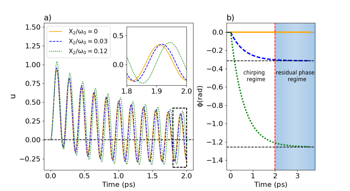
Figure 2: (color online) Calculations for representative parameter values. Frequency $\omega_{0}/(2\pi)=5.5$ THz, $X_{1}/\omega_{0}=0.5$, $\tau_{1}=0.7$ ps, $\tau_{2}=0.6$ ps, and $\gamma^{-1}=5$ ps, and for different strengths of the lattice feedback term $X_{2}$. $X_{2}=0$ corresponds to the phenomenological theory [46]. (a) Coherent phonon displacement $u(t)$, see Eqs. (8) and (9) and the associated text. The inset, a blow-up of the dashed rectangle, shows signature of the finite phase $\phi$ for different values of $X_{2}$. (b) The effects of the feedback at different time scales. At short times ($t\lesssim\tau_{2}$) a finite $X_{2}$ leads to chirping. At long times ($t\gg\tau_{2}$) it leads to a finite phase $\phi$, see also inset in (a). $\tau_{2}$ is defined in Eq. (5).

At face value, the above is a five parameter description of the coherent phonon. However, if the microscopic prescription is followed, $(X_{1},X_{2},\tau_{1},\tau_{2})$ can be obtained from the phenomenological parameters $T_{H}$ and $\tau_{e}$ defined in Eq. (2) by using the approximate relations of Eq. (5). Furthermore, if the theory to $\mathcal{O}(\lambda^{2})$ is quantitatively sufficient, then $\gamma^{-1}$ is the equilibrium phonon lifetime measured by, say, Raman response.

(iii) For $t\lesssim\tau_{2}$ the feedback $\Phi(t)$ describes temporal variation of the oscillation frequency, i.e., chirping, with a frequency variation $\Delta\omega_{0}\sim-X_{2}/2$, see Fig. 2. On the other hand, for $t\gg\tau_{2}$ we get a finite residual phase $\phi\equiv\Phi(t\rightarrow\infty)=-X_{2}\tau_{2}/2$, see Fig. 2. Note, even if $\left|\Delta\omega_{0}\right|/\omega_{0}\ll 1$ and the chirping is not experimentally observable at low fluence, the phase $\phi=(\Delta\omega_{0}/\omega_{0})(\omega_{0}\tau_{2})$ can be substantial since it involves the large parameter $\omega_{0}\tau_{2}$, c.f., Eq. (7). Note, the time dependent phase $\Phi(t)$ is qualitatively different from a constant phase that is usually discussed in the literature.

The chirping discussed here is related to the temperature, and hence, to the time dependence of the phonon frequency due to electron-phonon interaction. This is to be contrasted with other mechanisms of chirping discussed in the literature such as that due to phonon anharmonicity [15] and carrier diffusion [52; 53; 17].

(iv) Equilibrium Raman spectroscopy of BaFe₂As₂ shows that the $A_{1g}$ phonon frequency softens with increasing temperature [56]. Simultaneously, the phonon lifetime [56] has an atypical temperature dependence across the magnetic transition of BaFe₂As₂ which is very reminiscent of the $T$-dependence of resistivity [57], implying that the phonon temperature dependencies are likely due to interaction with the electrons. Thus, from these equilibrium trends, we conclude that $X_{2}>0$, and we predict that the coherent $A_{1g}$ phonon of BaFe₂As₂ will show red-shifted chirp at sufficiently high fluence.

(v) Since in our theory the frequency shift $\Delta\omega_{0}$ and the residual phase $\phi$ both depend on $X_{2}$, an important conclusion is that red-shifted (blue shifted) chirp is accompanied by negative (positive) residual phase. Note, the above expectation is indeed correct for the $A_{1g}$ coherent phonon of BaFe₂As₂, which softens with increasing temperature, and for which a negative phase $\phi=-0.1\pi$ has been reported [30; 31], see also the discussion in Sec. IV.

IV Quantitative description of the $A_{1g}$ coherent phonon in BaFe₂As₂

In this section, we apply the theory quantitatively to the coherent $A_{1g}$ phonon of the strongly correlated metal BaFe₂As₂, and we compare the theory results with a recent time-resolved x-ray study [31], see Fig 3. BaFe₂As₂ is the parent compound of a class of high temperature superconductors that also have rather interesting magnetic and nematic properties [58]. The $A_{1g}$ coherent phonon in this system, associated with the motion of the As atoms, has also been widely studied using a variety of pump-probe techniques [30; 31; 28; 26], including time-resolved x-ray spetcroscopy [31]which provides the most direct information about the As motion. The electronic properties of the BaFe₂As₂ are known [59] to be very sensitive to the As height, which makes the study of the coherent phonon motion all the more interesting.

Our overall goal in this section is to check to what extent a microscopic tight-binding model, that has been successfully used to understand equilibrium properties, can be used to describe the transient temperature dependencies involved in a pump-probe setting. Such an exercise is a step in the direction of extracting information about equilibrium properties from a pump-probe setup.

As a first, step we define the various parameters that we use to describe BaFe₂As₂ with the microscopic Hamiltonian of Eq. (II). We take the electronic kinetic part $\epsilon_{ab}(\textbf{k})$ from Ref. [60], which itself is obtained as a tight-binding fit of the LDA band structure onto a basis of five $d$ Fe orbitals [61]. Note, this particular set of tight-binding parameters has been used widely in the literature. Relatively less detailed information is currently available concerning the orbitally resolved electron-phonon matrix elements $C(\textbf{k})_{ab}$ of Eq. (II). However, it is well-accepted that an increase of the dimensionless arsenic height $u=\langle b^{\dagger}+b\rangle$ is accompanied by a reduction of the hopping-integrals and the bandwidths [62] since the hopping of the electrons between Fe atoms can also be mediated by the As atoms. Taking into account this physical expectation, we found that a simple way to model the electron-phonon matrix elements is to assume

$$C({\bf k})_{ab}=-[t_{nn}]_{ab}(\textbf{k}),$$ (10)

where $[t_{nn}]_{ab}$ is the diagonal nearest-neighbour entries of the tight-binding parameters $\epsilon_{ab}(\textbf{k})$. Thus, in our scheme the entire electron-phonon coupling is ultimately described by a single additional dimensionless parameter $\lambda$ which can later be absorbed in an overall scaling factor between the calculated $u(t)$ and the experimental x-ray intensity (see also the discussion following Eq. (13) below).

As a second step, we describe the calculation of the out-of-equilibrium force $F(t)$ (see also the discussion in the paragraph following Eq. (2)) to first order in $\lambda$. This involves the calculation of the thermal average of the weighted electron density operator. From Eq. (3) we get

$$\begin{split}\langle\hat{O}\rangle_{\mathcal{H}_{0},T}&\equiv\frac{\lambda}{\mathcal{N}}\sum_{{\bf k},a,b,\sigma}C({\bf k})_{ab}\langle c^{\dagger}_{{\bf k}a\sigma}c_{{\bf k}b\sigma}\rangle_{\mathcal{H}_{0},T}\\ &=\frac{\lambda}{\mathcal{N}}\sum_{{\bf k},\nu,\sigma}\tilde{C}({\bf k})_{\nu\nu}n_{F}\big{[}\xi_{\nu}(\textbf{k})-\mu(T),T\big{]},\end{split}$$ (11)

where the last equality is written in the band basis. Here $n_{F}$ is the Fermi function, $\xi_{\nu}(\textbf{k})$ is the energy of an electron in the band $\nu$ with momentum k, $\tilde{C}({\bf k})_{\nu\nu}$ is the electron-phonon matrix elements in the band basis, and $\mu(T)$ is the chemical potential at the transient temperature $T(t)$ at time $t$. We assume that there is no electronic diffusion [27], and that the particle number is conserved during the pump-probe cycle, which is consistent with the conclusions of a recent time-resolved photoemission study [30]. We divide the Brillouin zone into a ($10\times 10\times 10$) grid, and diagonalize $\mathcal{H}_{0}$ at each point of the grid to obtain the electronic dispersion $\xi_{\nu}(\textbf{k})$. The chemical potential is then calculated by solving the particle number conservation equation numerically. In Fig. 3 (a) we show the result of our calculation of $\langle\hat{O}\rangle_{\mathcal{H}_{0},T}$ for temperatures ranging from 0 to 3500 $\rm{(K)}$. This $T$-dependence can be transformed into a time dependence using Eq. (2) provided we have an estimate of the phenomenological parameters $(T_{H},\tau_{e})$ at each pump fluence. Henceforth, the base temperature is taken as $T_{L}=140$ K. The solid (black) line of Fig. 3 (b) gives such a transformation $\langle\hat{O}\rangle_{\mathcal{H}_{0},T}\rightarrow\langle\hat{O}\rangle(t)$ for a representative value of $(T_{H},\tau_{e})$. The resulting time dependence can be modeled by a single decaying exponential using Eq. (5). This leads to an estimate of $(X_{1},\tau_{1})$ for each pump fluence, see dashed (red) line of Fig. 3 (b).

cc

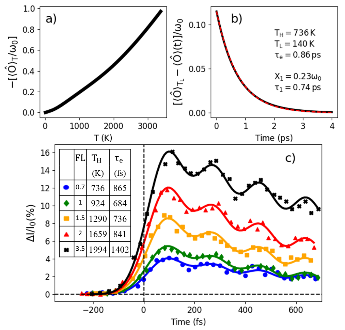
Figure 3: (color online) Quantitative description of the $A_{1g}$ coherent phonon (frequency $\omega_{0}/(2\pi)=5.5$ THz) of BaFe₂As₂, and comparison with experiment [31]. (a) Calculated equilibrium expectation value of the weighted electron density $\langle\hat{O}\rangle_{T}$ for $\lambda=$ 0.25. (b) Solid (black) line: The $T$-dependence in (a) is transformed into a time dependence using Eq. (2) for representative values of the phenomenological parameters $(T_{H},\tau_{e})$. Base temperature $T_{L}=140$ K. Dashed (red) line: Fit using Eq. (5), and estimate of $(X_{1},\tau_{1})$. (c) Solid lines: temporal variation of x-ray form factor calculated using Eq. (8) at different fluences (FL in mJ/cm${}^{2})$. The table gives estimates of $(T_{H},\tau_{e})$ used in the calculation. The fit uses $\gamma^{-1}=5$ ps, which is the equilibrium lifetime [56]. Symbols represent data points extracted from Ref. [31].

Note, the above step should not be construed as a mere replacement of two phenomenological parameters $(X_{1},\tau_{1})$ by two other phenomenological parameters $(T_{H},\tau_{e})$. This is because in our scheme the estimation of $(X_{1},\tau_{1})$ at each fluence is obtained via the evaluation of $\langle\hat{O}\rangle_{\mathcal{H}_{0},T}$ from the microscopic Hamiltonian Eq. (II) whose parameters are themselves fluence independent. Thus, the modeling is highly constrained, and it is not obvious that the $(X_{1},\tau_{1})$ needed for a given fluence can be obtained in our scheme for reasonable values of $(T_{H},\tau_{e})$ once the Hamiltonian is fixed. One way to appreciate the nontrivial step involved in our quantitative modeling is to note that our scheme can provide meaningful $(T_{H},\tau_{e})$ only if $\langle\hat{O}\rangle_{\mathcal{H}_{0},T}$ is a monotonically increasing function of temperature. On the other hand, such a property is a priori not guaranteed. Likewise, if the slope of the function $\langle\hat{O}\rangle_{\mathcal{H}_{0},T}$ is too large/small it would lead to values of $T_{H}$ that are too small/large compared to the estimates currently available from time-resolved photoemission studies [30].

In the third step we discuss the relevance of the $\lambda^{2}$ contribution to the force $F(t)$ that is implied in the experiment of Ref. [31; 30]. This contribution can be estimated from the following argument. To $\lambda^{2}$ accuracy, $\pi(T)$ can also be identified as the equilibrium phonon self-energy whose $T$-dependence can be inferred from equilibrium Raman measurement of $\omega_{0}(T)$ [56]. For $T_{L}=140$ K and $T_{H}\sim 500$ K, an extrapolation of $\omega_{0}(T)$ reported in Ref. [56] gives $\Delta\omega_{0}=0.4$ THz, and therefore $\frac{X_{2}}{\omega_{0}}\approx 0.01$, see Eq. (9). This small fraction implies that the $\lambda^{2}$ contribution to the force $F(t)$ is unimportant for the fluences used in Ref. [31]. Nevertheless, for the fits we kept the phase $\Phi(t)$ generated by the feedback effect, and we used the expression

$$u(t)=(X_{1}/\omega_{0})(\operatorname{e}^{-t/\tau_{1}}-\operatorname{e}^{-\gamma t}\cos[\omega_{0}t+\Phi(t)]),$$ (12)

by setting $\frac{X_{2}}{\omega_{0}}\rightarrow$ 0 in Eq. (8). To model $\Phi(t)$ we assume that it is fluence independent and that the experimentally reported phase $\phi=-0.1\pi$ [31; 30] can be identified with $\Phi(t\rightarrow\infty)=-X_{2}\tau_{2}/2$ (see Eq. (9)), from which we get $\tau_{2}\approx 800\,\rm{fs}$. Note also, for time $t\lesssim\tau_{e}$ the quality of the fit is marginally affected by including the feedback $\Phi(t)$ term.

Thus, following the above three steps we are able to compute $u(t)$ for a given fluence provided we have an estimate of $(T_{H},\tau_{e})$.

Finally, we compare the calculated arsenic displacement $u(t)$ with that measured in time resolved x-ray scattering [31] for a fluence range of $0.7$ to $3.5\,\rm{(mJ/cm^{2})}$. The intensity is convolved with a Gaussian pulse to account for the limited time resolution [31]. In the kinematic approximation [31] the variation of the intensity is proportional to the arsenic displacement and is given by

$$\frac{\Delta I}{I_{0}}(t)=\frac{B}{\tau_{r}\sqrt{\pi}}\int^{\infty}_{0}e^{-(\frac{t-\tau}{\tau_{r}})^{2}}u(\tau)d\tau,$$ (13)

where $I_{0}$ is the equilibrium intensity, $\Delta I$ is the variation of intensity out of equilibrium, $\tau_{r}\approx 96\,\rm{fs}$ is the experimental resolution of the probe-pulse, and $u(t)$ is computed using Eq. (12) following the three steps mentioned above. $B$ is a dimensionless proportionality constant, independent of fluence, that sets the overall scale of the theoretically evaluated $\Delta I/I_{0}$ with respect to the experimentally measured ones. Physically, $B$ is related to the change of the relevant x-ray form factor with the As atomic position. Within our scheme the constant $B$ and the dimensionless electron-phonon coupling $\lambda$ cannot be estimated separately. We find that best fits are obtained for $\lambda B=$ 4.9. In Fig. 3 (c) we compare the calculated $\Delta I/I_{0}$ (lines) with the data of Ref. [31] (solid symbols).

From Fig. 3(c) we conclude that the two-parameter fit is quite reasonable, given the simplicity of the starting model. Furthermore, our estimation of $(T_{H},\tau_{e})$, given in the inset of Fig. 3 (c), compares well with the experimental estimations given in Ref. [30]. The above attempt at a quantitative description is an important step towards making connection between equilibrium microscopic description of electrons with out-of-equilibrium pump-probe data. Note, the above calculation does not include temperature dependencies of the single electron properties arising due to electron-electron interaction. While such interaction effects can be incorporated in the current formalism, it is beyond the scope of the current work.

V Conclusions

We developed a microscopic theory of displacive coherent phonons driven by laser heating of carriers. Our theory captures physics beyond the standard phenomenological description, namely the modification of the electronic energy levels due to the phonon excitation, and how this change feeds back on the phonon dynamics. This effect of electron-phonon interaction leads to chirping at short time scales, and at long times it appears as a finite phase in the oscillatory signal. We successfully applied the theory to the $A_{1g}$ coherent phonon of BaFe₂As₂, thereby demonstrating that pump-probe data can be related to microscopic quantities and eventually to equilibrium physics. We explained the origin of the phase in the oscillatory signal reported in recent experiments [30; 31] on this system, and we predict that it will exhibit red-shifted chirping at larger fuence.

Appendix A Structure of $\Pi_{T(t)}(t-t^{\prime})$

The response function used in the main text is defined by

$$\Pi_{T(t)}(t-t^{\prime})\equiv i\theta(t-t^{\prime})\langle\left[\hat{O}(t^{\prime}),\hat{O}(t)\right]\rangle_{\mathcal{H}_{0},T(t)},$$ (14)

where $\hat{O}\equiv(\lambda/\mathcal{N})\sum_{{\bf k},a,b,\sigma}C({\bf k})_{ab}c^{\dagger}_{{\bf k}a\sigma}c_{{\bf k}b\sigma}$ is the weighted electron density operator, $\mathcal{H}_{0}\equiv\mathcal{H}(\lambda=0)$, and the Hamiltonian $\mathcal{H}$ is given by Eq. (1) in the main text. In equilibrium $\Pi_{T(t)}(t-t^{\prime})$ is a function of $(t-t^{\prime})$ only, but this is no longer the case out-of-equilibrium. Here, we discuss the $t$ and $t^{\prime}$ dependencies of $\Pi_{T(t)}(t-t^{\prime})$. We write the response function in the Lehmann representation where the time structure can be made explicit

$$\begin{split}\Pi_{T(t)}(t-t^{\prime})&=i\theta(t-t^{\prime})\sum_{n,m}\lvert\bra{n}\hat{O}\ket{m}\rvert^{2}e^{i(t-t^{\prime})(E_{n}-E_{m})}\\ &\times\bigg{(}e^{-\beta(t)E_{m}}-e^{-\beta(t)E_{n}}\bigg{)},\end{split}$$ (15)

where $E_{n}$ and $\ket{n}$ are respectively a complete set of eigenenergies and eigenstates of the Hamiltonian $\mathcal{H}_{0}$. We see from (15) that the response function is a function of the time difference ($t-t^{\prime}$), and that the explicit time $t$ dependence enters only through the electronic temperature $T(t)$. We can then define the Fourier transform of the response function with respect to the time difference ($t-t^{\prime}$) evaluated at the electronic temperature $T(t)$

$$\begin{split}\Pi_{T(t)}(\Omega)&=\sum_{n,m}\lvert\bra{n}\hat{O}\ket{m}\rvert^{2}\frac{1}{E_{n}-E_{m}-\Omega+i\eta}\\ &\times\bigg{(}e^{-\beta(t)E_{n}}-e^{-\beta(t)E_{m}}\bigg{)},\end{split}$$ (16)

where $\eta$ is an arbitrarily small positive constant that ensures the convergence of the Fourier transform. By inspection, we see that the response function in frequency domain (16) is the equilibrium retarded phonon self-energy evaluated to second order in the electron-phonon interaction ($\lambda^{2}$) at temperature $T(t)=1/\beta(t)$.

Appendix B Solution of the differential equation for $u(t)$

As discussed in the main text, if the instantaneous out-of-equilibrium force $f(t)$ is evaluated to second order in electron-phonon interaction the theory captures the modification of the electronic dispersion due to the coherent phonon excitation, and how that feeds back upon the dynamics of the phonon itself. Taking this feedback into account the differential equation governing the atomic displacement $u(t)$ is given by [see Eqs. (4) and (6) in main text]

$$\left(\partial_{t}^{2}+2\gamma\partial_{t}+\omega_{0}^{2}\right)u=f(t)=\omega_{0}\left(X_{1}\operatorname{e}^{-t/\tau_{1}}+uX_{2}\operatorname{e}^{-t/\tau_{2}}\right).$$ (17)

The parameters $(\omega_{0},X_{1},X_{2},\gamma,\tau_{1/2})$ are defined in the main text. Here we discuss the solution of the above differential equation subject to the initial conditions $u(0)=0$ and $\partial_{t}u(0)=0$, and in the experimentally relevant limit of $[\gamma/\omega_{0},1/(\omega_{0}\tau_{1/2})]\rightarrow 0$. The equation of motion (17) is linear, the solution is then the sum of the homogeneous and particular solution $u(t)=y_{h}(t)+y_{p}(t)$. We first discuss the homogeneous solution, then following the same method we give the particular solution. We start from the following ansatz for the homogeneous solution

$$\begin{split}y_{h}(t)&=\sum_{n=0}^{\infty}a_{n}e^{k_{n}t}+cc,\\ \end{split}$$ (18)

with $k_{n}=i\omega_{1}-\gamma-n/\tau_{2}$, and $\omega_{1}=\sqrt{(\omega_{0})^{2}-\gamma^{2}}$. We insert (18) into the homogeneous equation, and obtain an equation for the coefficients $a_{n}$

$$\begin{split}a_{n}(k_{n}^{2}+2\gamma_{0}k_{n}+(\omega_{0})^{2})&=\omega_{0}X_{2}a_{n-1},\\ a_{0}(k_{0}^{2}+2\gamma_{0}k_{0}+(\omega_{0})^{2})&=0.\end{split}$$ (19)

Since $k_{0}$ satisfies the equation $(k_{0}^{2}+2\gamma_{0}k_{0}+(\omega_{0})^{2})=0$, $a_{0}$ is then an arbitrary complex constant. We solve the coupled equation (19), and obtain for $a_{n}$

$$\begin{split}a_{n}&=a_{0}(\omega_{0}X_{2})^{n}\prod_{m=1}^{n}\frac{1}{k_{m}^{2}+2\gamma k_{m}+\omega_{0}^{2}}\\ &=\frac{a_{0}}{n!}\left(\frac{iX_{2}\tau_{2}}{2\omega_{1}}\right)^{n}\prod_{m=1}^{n}\frac{1}{1+(2i)(m/\tau_{2}\omega_{0})}\\ &\approx\frac{a_{0}}{n!}\left(\frac{iX_{2}\tau_{2}}{2\omega_{0}}\right)^{n},\end{split}$$ (20)

where in the last step we took the limit $[\gamma/\omega_{0},1/(\omega_{0}\tau_{2})]\rightarrow 0$, the homogeneous solution then reads

$$\begin{split}y_{h}(t)&=a_{0}e^{(i\omega_{0}-\gamma)t}\sum_{n}^{\infty}\frac{1}{n!}\left(\frac{iX_{2}\tau_{1}}{2\omega_{0}}e^{-t/\tau_{2}}\right)^{n}+c.c.\\ &=a_{0}e^{-\gamma t}\bigg{(}e^{i\omega_{0}+i\frac{X_{2}\tau_{2}}{2\omega_{0}}e^{-t/\tau_{2}}}\bigg{)}+c.c.,\end{split}$$ (21)

We replace $a_{0}=\frac{1}{2}Ae^{i\psi}$ and finally obtain for the homogeneous solution

$$y_{h}(t)=Ae^{-\gamma t}\cos{\bigg{(}\omega_{0}t+\frac{X_{2}\tau_{2}}{2\omega_{0}}e^{-t/\tau_{2}}+\psi\bigg{)}},$$ (22)

where $(A,\psi)$ are arbitrary constants to be determined from the initial conditions. We follow the same method to find the particular solution, we start from the ansatz

$$y_{p}(t)=\sum_{n=0}^{\infty}b_{n}e^{\alpha_{n}t},\\$$ (23)

with $\alpha_{n}=-1/\tau_{1}-n/\tau_{2}$. We insert (23) into the equation of motion (17), and get an equation for the coefficients $b_{n}$

$$\begin{split}b_{n}(\alpha_{n}^{2}+2\gamma_{0}\alpha_{n}+(\omega_{0})^{2})&=\omega_{0}X_{2}a_{n-1},\\ b_{0}(\alpha_{0}^{2}+2\gamma_{0}\alpha_{0}+(\omega_{0})^{2})&=\omega_{0}X_{1}.\end{split}$$ (24)

We solve the coupled equations and obtain

$$\begin{split}b_{n}&=\frac{\omega_{0}X_{1}(\omega_{0}X_{2})^{n}}{(1/\tau_{1})^{2}-2\gamma(1/\tau_{1})+(\omega_{0})^{2}}\prod_{m=1}^{n}\frac{1}{\alpha_{m}^{2}+2\gamma\alpha_{m}+\omega_{0}^{2}}\\ &\approx\frac{X_{1}}{\omega_{0}}\left(\frac{X_{2}}{\omega_{0}}\right)^{n},\end{split}$$ (25)

where in the last step we took the limit $[\gamma/\omega_{0},1/(\omega_{0}\tau_{1/2})]\rightarrow 0$, the particular solution then reads

$$\begin{split}y_{p}(t)&=\frac{X_{1}}{\omega_{0}}e^{-t/\tau_{1}}\sum_{n}^{\infty}\left(\frac{X_{2}e^{-t/\tau_{2}}}{\omega_{0}}\right)^{n}\\ &=\frac{X_{1}}{\omega_{0}-X_{2}e^{-t/\tau_{2}}}e^{-t/\tau_{1}}.\end{split}$$ (26)

We use the initial conditions $u(0)=0$ and $\partial_{t}u(0)=0$ to calculate the arbitrary constants $(A,\psi)$. The solution in the limit $[\gamma/\omega_{0},1/(\omega_{0}\tau_{1/2})]\rightarrow 0$ reads

$$\begin{split}u(t)&=\frac{X_{1}}{\omega_{0}-X_{2}e^{-t/\tau_{2}}}e^{-t/\tau_{1}}\\ &-\frac{X_{1}}{\omega_{0}-X_{2}}e^{-\gamma t}\cos{\bigg{(}\omega_{0}t+\frac{X_{2}\tau_{2}}{2\omega_{0}}\big{(}e^{-t/\tau_{2}}-1\big{)}\bigg{)}},\end{split}$$ (27)

where we finally recognize Eq (8) of the main text.

References

- [1] For a recent review see, e.g., C. Giannetti, M. Capone, D. Fausti, M. Fabrizio, F. Parmigiani, and D. Mihailovic, Adv. Phys. 65, 58 (2016).
- [2] U. Bovensiepen, J. Phys. Condens. Matter 19, 083201 (2007).
- [3] C. L. Smallwood, R. A. Kaindl, and A. Lanzara, EPL 115, 27001 (2016).
- [4] S. De Si lvestri, J. G. Fujimoto, E. P. Ippen, E. B. Gamble, L. R. Williams, and K. A. Nelson, Chem. Phys. Lett. 116, 146 (1985).
- [5] T. K. Cheng, S. D. Brorson, A. S. Kazeroonian, J. S. Moodera, G. Dresselhaus, M. S. Dresselhaus, and E. P. Ippen, Appl. Phys. Lett. 57, 1004 (1990).
- [6] G. C. Cho, W. Kütt, and H. Kurz, Phys. Rev. Lett. 65, 764 (1990).
- [7] For a review see, e.g., K. Ishioka, and O. V. Misochko, Springer Ser. Chem. Phys. 98, 23 (2010).
- [8] H. Hübener, U. De Giovannini, and A. Rubio, Nano Lett. 18, 1535 (2018).
- [9] T. Oka and S. Kitamura, Annu. Rev. Condens. Matter Phys. 10, 387 (2019).
- [10] S. Hunsche, K. Wienecke, T. Dekorsy, and H. Kurz, Phys. Rev. Lett. 75, 1815 (1995).
- [11] D. M. Riffe and A. J. Sabbah, Phys. Rev. B 76, 085207 (2007), and references therein.
- [12] E. M. Bothschafter, A. Paarmann, E. S. Zijlstra, N. Karpowicz, M. E. Garcia, R. Kienberger, and R. Ernstorfer, Phys. Rev. Lett. 110, 067402 (2013).
- [13] M. Hase, K. Mizoguchi, H. Harima, and S. Nakashima, Appl. Phys. Lett. 69, 2474 (1996).
- [14] M. F. DeCamp, D. A. Reis, P. H. Bucksbaum, and R. Merlin, Phys. Rev. B 64, 092301 (2001).
- [15] M. Hase, M. Kitajima, S.-I. Nakashima, and K. Mizoguchi, Phys. Rev. Lett. 88, 067401 (2002).
- [16] O.V. Misochko, M. Hase, K. Ishioka, and M. Kitajima, Phys. Rev. Lett. 92, 197401 (2004).
- [17] D. M. Fritz, D. A. Reis, B. Adams, R. A. Akre, J. Arthur, C. Blome, P. H. Bucksbaum, A. L. Cavalieri, S. Engemann, S. Fahy, R. W. Falcone, P. H. Fuoss, K. J. Gaffney, M. J. George, J. Hajdu, M. P. Hertlein, P. B. Hillyard, M. Horn-von Hoegen, M. Kammler, J. Kaspar, R. Kienberger, P. Krejcik, S. H. Lee, A. M. Lindenberg, B. McFarland, D. Meyer, T. Montagne, É. D. Murray, A. J. Nelson, M. Nicoul, R. Pahl, J. Rudati, H. Schlarb, D. P. Siddons, K. Sokolowski-Tinten, Th. Tschentscher, D. von der Linde, and J. B. Hastings, Science 315, 633 (2007).
- [18] S. L. Johnson, P. Beaud, C. J. Milne, F. S. Krasniqi, E. S. Zijlstra, M. E. Garcia, M. Kaiser, D. Grolimund, R. Abela, and G. Ingold, Phys. Rev. Lett. 100, 155501 (2008).
- [19] E. Papalazarou, J. Faure, J. Mauchain, M. Marsi, A. Taleb-Ibrahimi, I. Reshetnyak, A. van Roekeghem, I. Timrov, N. Vast, B. Arnaud, and L. Perfetti, Phys. Rev. Lett. 108, 256808 (2012).
- [20] M. Hase, K. Ishioka, J. Demsar, K. Ushida, and M. Kitajima, Phys. Rev. B 71, 184301 (2005).
- [21] J. M. Chwalek, C. Uher, J. F. Whitaker, G. A. Mourou, J. Agostinelli, and M. Lelental, Appl. Phys. Lett. 57, 1696 (1990).
- [22] W. Albrecht, T. Kruse, and H. Kurz, Phys. Rev. Lett. 69, 1451 (1992).
- [23] I. Bozovic, M. Schneider, Y. Xu, R. Sobolewski, Y. H. Ren, G. Lüpke, J. Demsar, A. J. Taylor, and M. Onellion, Phys. Rev. B 69, 132503 (2004).
- [24] F. Novelli, G. Giovannetti, A. Avella, F. Cilento, L. Patthey, M. Radovic, M. Capone, F. Parmigiani, and D. Fausti, Phys. Rev. B 95, 174524 (2017).
- [25] B. Mansart, D. Boschetto, A. Savoia, F. Rullier-Albenque, A. Forget, D. Colson, A. Rousse, and M. Marsi, Phys. Rev. B 80, 172504 (2009).
- [26] B. Mansart, D. Boschetto, A. Savoia, F. Rullier-Albenque, F. Bouquet, E. Papalazarou, A. Forget, D. Colson, A. Rousse, and M. Marsi, Phys. Rev. B 82, 024513 (2010).
- [27] D. H. Torchinsky, J. W. McIver, D. Hsieh, G. F. Chen, J. L. Luo, N. L. Wang, and N. Gedik, Phys. Rev. B 84, 104518 (2011).
- [28] K.W. Kim, A. Pashkin, H. Schäfer, M. Beyer, M. Porer, T.Wolf, C. Bernhard, J. Demsar, R. Huber, and A. Leitenstorfer, Nat. Mater. 11, 497 (2012).
- [29] I. Avigo, R. Cortés, L. Rettig, S. Thirupathaiah, H. S. Jeevan, P. Gegenwart, T. Wolf, M. Ligges, M. Wolf, J. Fink and U. Bovensiepen1, J. Phys. Condens. Matter 25, 094003 (2013).
- [30] L. X. Yang, G. Rohde, T. Rohwer, A. Stange, K. Hanff, C. Sohrt, L. Rettig, R. Cortés, F. Chen, D. L. Feng, T. Wolf, B. Kamble, I. Eremin, T. Popmintchev, M. M. Murnane, H. C. Kapteyn, L. Kipp, J. Fink, M. Bauer, U. Bovensiepen, and K. Rossnagel, Phys. Rev. Lett. 112, 207001 (2014).
- [31] L. Rettig, S. O. Mariager, A. Ferrer, S. Grübel, J. A. Johnson, J. Rittmann, T. Wolf, S. L. Johnson, G. Ingold, P. Beaud, and U. Staub, Phys. Rev. Lett. 114, 067402 (2015).
- [32] S. Gerber, K. W. Kim, Y. Zhang, D. Zhu, N. Plonka, M. Yi, G. L. Dakovski, D. Leuenberger, P.S. Kirchmann, R. G. Moore, M. Chollet, J. M. Glownia, Y. Feng, J.-S. Lee, A. Mehta, A. F. Kemper, T. Wolf, Y.-D. Chuang, Z. Hussain, C.-C. Kao, B. Moritz, Z.-X. Shen, T. P. Devereaux and W.-S. Lee, Nat. Commun. 6, 7377 (2015).
- [33] S. Gerber, S.-L. Yang, D. Zhu, H. Soifer, J. A. Sobota, S. Rebec, J. J. Lee, T. Jia, B. Moritz, C. Jia, A. Gauthier, Y. Li, D. Leuenberger, Y. Zhang, L. Chaix, W. Li, H. Jang, J.-S. Lee, M. Yi, G. L. Dakovski, S. Song, J. M. Glownia, S. Nelson, K. W. Kim, Y.-D. Chuang, Z. Hussain, R. G. Moore, T. P. Devereaux, W.-S. Lee, P. S. Kirchmann, Z.-X. Shen, Science 357, 71 (2017).
- [34] K. Kenji, M. Hase, H. Harima, S.-I. Nakashima, M. Tani, K. Sakai, H. Negishi, and M. Inoue, Phys. Rev. B 58, R7484(R) (1998).
- [35] J. Demsar, K. Biljaković, and D. Mihailovic, Phys. Rev. Lett. 83, 800 (1999).
- [36] Y. Toda, K. Tateishi, and S. Tanda, Phys. Rev. B 70, 033106 (2004).
- [37] H. Schaefer, V. V. Kabanov, and J. Demsar, Phys. Rev. B 89, 045106 (2014).
- [38] F. Schmitt, P. S. Kirchmann, U. Bovensiepen, R. G. Moore, J.-H. Chu, D. H. Lu, L. Rettig, M. Wolf, I. R. Fisher, and Z.-X. Shen, New J. Phys. 13, 063022 (2011).
- [39] L. Perfetti, P. A. Loukakos, M. Lisowski, U. Bovensiepen, M. Wolf, H. Berger, S. Biermann, and A. Georges, New J. Phys. 10, 053019 (2008).
- [40] B. Mansart, D. Boschetto, S. Sauvage, A. Rousse, and M. Marsi, EPL 92, 37007 (2010).
- [41] R. Mankowsky, M. Först, T. Loew, J. Porras, B. Keimer, and A. Cavalleri, Phys. Rev. B 91, 094308 (2015).
- [42] M.-C. Lee, C. H. Kim, I. Kwak, C. W. Seo, C. H. Sohn, F. Nakamura, C. Sow, Y. Maeno, E.-A. Kim, T. W. Noh, and K. W. Kim, arXiv:1712.03028.
- [43] A. Q. Wu, X. Xu, and R. Venkatasubramanian, Appl. Phys. Lett. 92, 011108 (2008).
- [44] N. Kamaraju, S. Kumar, and A. K. Sood, EPL 92, 47007 (2010).
- [45] O. V. Misochko, J. Flock, and T. Dekorsy, Phys. Rev. B 91, 174303 (2015).
- [46] H. J. Zeiger, J. Vidal, T. K. Cheng, E.P. Ippen, G. Dresselhaus, and M. S. Dresselhaus, Phys. Rev. B 45, 768 (1992).
- [47] A. V. Kuznetsov and C. J. Stanton, Phys. Rev. Lett. 73, 3243 (1994).
- [48] G. A. Garrett, T. F. Albrecht, J. F. Whitaker, and R. Merlin, Phys. Rev. Lett. 77, 3661 (1996).
- [49] R. Merline, Solid State Commun. 102, 207 (1997).
- [50] T. E. Stevens, J. Kuhl, and R. Merlin, Phys. Rev. B 65, 144304 (2002).
- [51] I. I. Mazin, A. I. Liechtenstein, O. Jepsen, O. K. Andersen, and C. O. Rodriguez, Phys. Rev. B 49, 9210 (1994).
- [52] P. Tangney and S. Fahy, Phys. Rev. Lett. 82, 4340 (1999).
- [53] P. Tangney and S. Fahy, Phys. Rev. B 65, 054302 (2002).
- [54] É. D. Murray, D. M. Fritz, J. K. Wahlstrand, S. Fahy, and D. A. Reis, Phys. Rev. B 72, 060301(R) (2005).
- [55] Y. Shinohara, K. Yabana, Y. Kawashita, J.-I. Iwata, T. Otobe, and G. F. Bertsch, Phys. Rev. B 82, 155110 (2010).
- [56] M. Rahlenbeck, G. L. Sun, D. L. Sun, C. T. Lin, B. Keimer, and C. Ulrich, Phys. Rev. B 80, 064509 (2009).
- [57] F. Rullier-Albenque, D. Colson, A. Forget, and H. Alloul, Phys. Rev. Lett. 103, 057001 (2009).
- [58] For a review on Fe-based superconductors see, e.g., D. C. Johnston, Adv. Phys. 59, 803 (2010).
- [59] See, e.g., T. Egami, B. V. Fine, D. Parshall, A. Subedi, and D. J. Singh, Adv. Condens. Matter Phys. 2010, 1 (2010).
- [60] For example, S. Graser, A. F. Kemper, T. A. Maier, H.-P. Cheng, P. J. Hirschfeld, and D. J. Scalapino, Phys. Rev. B 81, 214503 (2010).
- [61] Milan Tomić, Harald O. Jeschke, Roser Valenti, Phys. Rev. B 90, 195121 (2014).
- [62] K. Kuroki, H. Usui, S. Onari, R. Arita, and H. Aoki, Phys. Rev. B 79, 224511 (2009).