Flows and dynamos in a model of stellar radiative zones

Abstract

Stellar radiative zones are typically assumed to be motionless in standard models of stellar structure but there is sound theoretical and observational evidence that this cannot be the case. We investigate by direct numerical simulations a three-dimensional and time-dependent model of stellar radiation zones consisting of an electrically-conductive and stably-stratified anelastic fluid confined to a rotating spherical shell and driven by a baroclinic torque. As the baroclinic driving is gradually increased a sequence of transitions from an axisymmetric and equatorially-symmetric time-independent flow to flows with a strong poloidal component and lesser symmetry are found. It is shown that all flow regimes characterised with significant non-axisymmetric components are capable of generating self-sustained magnetic field. As the value of the Prandtl number is decreased and the value of the Ekman number is decreased flows become strongly time-dependent with progressively complex spatial structure and dynamos can be generated at lower values of the magnetic Prandtl number.

1 Introduction

It has long been known theoretically that radiative zones in rotating stars cannot be in static equilibrium (von Zeipel 1924). Instead the basic axisymmetric solution of the problem consists of a differential rotation and a rather weak meridional circulation driven by the centrifugal force in the presence of the Coriolis force (Schwarzschild 1947, Busse 1982, Spruit and Knobloch 1984). In more recent years, fluid motions and the possibility of magnetic field generation in stably stratified stellar radiative zones have gained considerable interest owing to increasingly detailed observations of stellar magnetic fields. To model radiative cores several numerical studies of baroclinically-driven flows in stably stratified rotating spheres have been published, notably (Rieutord 2006, Espinosa and Rieutord 2013, Hypolite and Rieutord 2014, Rieutord and Beth 2014). However, these studies have been restricted to modelling two-dimensional and steady axisymmetric flows and have been based on the Boussinesq approximation which does not account for the strong density variations typical for stably stratified regions in stars. Also the possibility of magnetic flux generation by dynamo action has not been considered in these papers.

These restrictions have been lifted in a recent study by Simitev and Busse (2017) who considered a non-axisymmetric and time-dependent model of baroclinic flows in rotating spherical fluid shells based on the anelastic approximation (Gough 1969, Braginsky and Roberts 1995, Lantz and Fan 1999). Simitev and Busse (2017) found a sequence of bifurcations from simple regular to complex irregular flows with increasing baroclinicity. Some of the transitions in this sequence were observed to exhibit hysteretic behaviour. They noted that with increasing baroclinicity the poloidal component of the flow grows relative to the dominant toroidal component and thus facilitates magnetic field generation. Simitev and Busse (2017) proceeded to report a non-decaying dynamo solution and suggested that self-sustained dynamo action of baroclinically-driven flows may allow for the possibility that magnetic fields in stably stratified stellar interiors are not necessarily of fossil origin as is often assumed.

In the present study, we essentially confirm and significantly extend the results presented in (Simitev and Busse 2017) by summarizing over 90 new hydrodynamic and hydromagnetic numerical simulations, 62 of which are explicitly included in the text. The results of (Simitev and Busse 2017) were restricted to fixed values for all model parameters apart from the baroclinicity parameter. In particular, the value of the Prandtl number was fixed to $\mathrm{Pr}=0.1$ which restricts the baroclinicity to a fairly modest value and only steady flows were thus reported. In addition, only a single steady dynamo was presented in (Simitev and Busse 2017) for an unrealistically large value of the magnetic Prandtl number. Here, we investigate a much larger region of the parameter space reaching in the directions of smaller values of the Prandtl number and of the magnetic Prandtl number and of smaller values of the Ekman number. We report one new hydrodynamic instability and we find essentially time-dependent flows. Another main goal of the present study is to determine which of the distinct baroclinically-driven flow states found are capable of generating self-sustained magnetic field and we are able to establish the existence of dynamo excitation in all states with non-axisymmetric flow components. The critical value of the magnetic Prandtl number for the onset of dynamo action is determined and the dynamo mechanism is elaborated.

2 Mathematical model

Our model of a stably-stratified stellar radiative zone is based on the anelastic approximation (Gough 1969, Braginsky and Roberts 1995, Lantz and Fan 1999) which is widely adopted for numerical simulations of convection in Solar and stellar interiors (Jones et al. 2011). Accordingly, we consider a perfect gas confined to a spherical shell rotating with a fixed angular velocity $\varOmega\hat{\mbox{\boldmath$k$}}$, where $\hat{\mbox{\boldmath$k$}}$ is the unit vector in the direction of the axis of rotation. A positive entropy contrast $\Delta S$ is imposed between its outer and inner surfaces at radii $r_{o}$ and $r_{i}$, respectively. We assume a gravity field proportional to $g/r^{2}$. To justify this choice consider the Sun, the star with the best-known physical properties. The Solar density drops from 150 g/cm³ at the centre to 20 g/cm³ at the core-radiative zone boundary (at $0.25R_{\odot}$) to only 0.2 at the tachocline (at $0.7R_{\odot}$). A crude piecewise linear interpolation shows that most of the mass is concentrated within the core. In this setting a hydrostatic polytropic reference state exists with profiles of density, temperature and pressure given by the expressions

$$\bar{\rho}=\rho_{c}\zeta^{n},\qquad\bar{T}=T_{c}\zeta,\qquad\bar{P}=P_{c}\zeta^{n+1},$$

respectively, where

$$\zeta=c_{0}+\frac{c_{1}}{r},\qquad\zeta_{o}=\frac{\eta+1}{\eta\exp(N_{\rho}/n)+1},$$

$$c_{0}=\frac{2\zeta_{o}-\eta-1}{1-\eta},\qquad c_{1}=\frac{(1+\eta)(1-\zeta_{o})}{1-\eta}^{2},$$

see (Jones et al. 2011). The parameters $\rho_{c}$, $P_{c}$ and $T_{c}$ are reference values of density, pressure and temperature at mid-shell. The gas polytropic index $n$, the density scale height $N_{\rho}$ and the shell radius ratio $\eta$ are defined further below. Since a rigidly rotating stellar interior can not exist, the deviation from such a state is described by the baroclinic parameter ${\mathrm{Z}}$, introduced below. This parameter is associated with the centrifugal force which balances the baroclinic torques (Busse 1982). Following Rieutord (2006) we neglect the distortion of the isopycnals caused by the centrifugal force. The governing anelastic equations of continuity, momentum, energy (entropy), and magnetic induction assume the form

$${\mbox{\boldmath$\nabla$}}{\mbox{\boldmath$\cdot$}}\bar{\rho}\mbox{\boldmath$u$}= \;0,$$ (1a)

$$\quad\quad\mbox{\boldmath$\nabla$}\mbox{\boldmath$\cdot$}\mbox{\boldmath$B$}= \;0,$$ (1b)

$$\upartial_{t}\mbox{\boldmath$u$}+({\mbox{\boldmath$\nabla$}}\times\mbox{\boldmath$u$})\times\mbox{\boldmath$u$}= \;-{\mbox{\boldmath$\nabla$}}\varPi-\frac{2}{\mathrm{Ek}}(\hat{\mbox{\boldmath$k$}}\times\mbox{\boldmath$u$})+\frac{\mathrm{R}}{\mathrm{Pr}}\frac{{S}}{r^{2}}\hat{\mbox{\boldmath$r$}}+\mbox{\boldmath$F$}_{\nu}$$

$$\;\qquad\quad+\frac{1}{\bar{\rho}}({\mbox{\boldmath$\nabla$}}\times\mbox{\boldmath$B$})\times\mbox{\boldmath$B$}-{\mathrm{Z}}(\overline{S}+S)\;\hat{\mbox{\boldmath$k$}}\times(\mbox{\boldmath$r$}\times\hat{\mbox{\boldmath$k$}}),$$ (1c)

$$\upartial_{t}S+\mbox{\boldmath$u$}{\mbox{\boldmath$\cdot$}}{\mbox{\boldmath$\nabla$}}{(\overline{S}+S)}= \;\frac{1}{\mathrm{Pr}\bar{\rho}\bar{T}}{\mbox{\boldmath$\nabla$}}{\mbox{\boldmath$\cdot$}}\bar{\rho}\bar{T}{\mbox{\boldmath$\nabla$}}S+\frac{c_{1}\mathrm{Pr}}{\mathrm{R}\bar{T}}\left(Q_{\nu}+\frac{1}{\mathrm{Pm}\bar{\rho}}Q_{j}\right),$$ (1d)

$$\upartial_{t}\mbox{\boldmath$B$}= \;{\mbox{\boldmath$\nabla$}}\times(\mbox{\boldmath$u$}\times\mbox{\boldmath$B$})+\mathrm{Pm}^{-1}\nabla^{2}\mbox{\boldmath$B$},$$ (1e)

where $S$ is the deviation from the background entropy profile

$$\overline{S}=\frac{\zeta(r)^{-n}-\zeta_{o}^{-n}}{\zeta_{o}^{-n}-\zeta_{i}^{-n}},$$

$u$ is the velocity vector, $B$ is the magnetic flux density, ${\mbox{\boldmath$\nabla$}}\varPi$ includes all terms that can be written as gradients, and $\mbox{\boldmath$r$}=r\hat{\mbox{\boldmath$r$}}$ is the position vector with respect to the center of the sphere (Jones et al. 2011, Simitev et al. 2015). The viscous force, the viscous heating and the Ohmic heating, given by

$$\mbox{\boldmath$F$}_{\nu}=(\rho_{c}/\bar{\rho}){\mbox{\boldmath$\nabla$}}{\mbox{\boldmath$\cdot$}}\mbox{\boldmath$\hat{S}$},\qquad Q_{\nu}=\mbox{\boldmath$\hat{S}$}{\mbox{\boldmath$:$}}\mbox{\boldmath$e$},\qquad Q_{j}=(\mbox{\boldmath$\nabla$}\times\mbox{\boldmath$B$})^{2},$$

respectively, are defined in terms of the deviatoric stress tensor

$$\hat{S}_{ij}=2\bar{\rho}(e_{ij}-e_{kk}\delta_{ij}/3),\qquad e_{ij}=(\upartial_{i}u_{j}+\upartial_{j}u_{i})/2,$$

where double-dots (:) denote a Frobenius inner product, and $\nu$ is a constant viscosity. The governing equations (1) have been non-dimensionalized with the shell thickness $d=r_{o}-r_{i}$ as unit of length, $d^{2}/\nu$ as unit of time, $\nu\sqrt{\mu_{0}\rho_{c}}/d$ as a unit of magnetic induction, and $\Delta S$, $\rho_{c}$ and $T_{c}$ as units of entropy, density and temperature, respectively. The system is then characterized by eight dimensionless parameters: the radius ratio, the polytropic index of the gas, the density scale number, the Prandtl number, the magnetic Prandtl number, the Rayleigh number, the Ekman number and the baroclinicity parameter

$$\eta=r_{i}/r_{o},\qquad n,\qquad N_{\rho}=\ln\big{(}\bar{\rho}(r_{i})/\bar{\rho}(r_{o})\big{)},\qquad\mathrm{Pr}={\nu}/{\kappa},\qquad$$

$$\mathrm{Pm}={\nu}/{\lambda},\qquad\mathrm{R}=-{gd^{3}\Delta S}/({\nu\kappa c_{p}}),\qquad\mathrm{Ek}={\nu}/(\varOmega d^{2}),\qquad{\mathrm{Z}}={\varOmega^{2}d^{4}\Delta S}/({\nu^{2}c_{p}}),$$

respectively, where $\kappa$ is a constant entropy diffusivity, $\lambda$ and $\mu_{0}$ are the magnetic diffusivity and permeability, and $c_{p}$ is the specific heat at constant pressure. Note, that the Rayleigh number assumes negative values in the present problem since the basic entropy gradient is reversed with respect to the case of buoyancy driven convection.

The poloidal-toroidal decomposition

$$\bar{\rho}\mbox{\boldmath$u$}={\mbox{\boldmath$\nabla$}}\times({\mbox{\boldmath$\nabla$}}\times\hat{\mbox{\boldmath$r$}}rv)+{\mbox{\boldmath$\nabla$}}\times\hat{\mbox{\boldmath$r$}}r^{2}w,$$

$$\mbox{\boldmath$B$}=\mbox{\boldmath$\nabla$}\times(\mbox{\boldmath$\nabla$}\times\hat{\mbox{\boldmath$r$}}h)+\mbox{\boldmath$\nabla$}\times\hat{\mbox{\boldmath$r$}}g,$$

is used to enforce the solenoidality of the mass flux $\bar{\rho}\mbox{\boldmath$u$}$ and of the magnetic flux density. This has the further advantages that the pressure gradient can be eliminated and scalar equations for the poloidal and the toroidal scalar fields, $v$ and $w$, are obtained by taking $\hat{\mbox{\boldmath$r$}}{\mbox{\boldmath$\cdot$}}{\mbox{\boldmath$\nabla$}}{\times{\mbox{\boldmath$\nabla$}}\times}$ and $\hat{\mbox{\boldmath$r$}}{\mbox{\boldmath$\cdot$}}{\mbox{\boldmath$\nabla$}}\times$ of equation (1c). Similarly equations for the poloidal and the toroidal scalar fields, $h$ and $g$, are obtained by taking $\hat{\mbox{\boldmath$r$}}{\mbox{\boldmath$\cdot$}}{\mbox{\boldmath$\nabla$}}\times$ and $\hat{\mbox{\boldmath$r$}}{\mbox{\boldmath$\cdot$}}$ of equation (1e). Except for the term with the baroclinicity parameter ${\mathrm{Z}}$ the resulting equations are identical to those described by Simitev et al. (2015). Assuming that entropy fluctuations are damped by convection in the region above $r=r_{o}$ we choose the boundary condition

$$S=0\quad\text{at }\quad r=\left\{\begin{array}[]{l}r_{i}\equiv\eta/(1-\eta)\,,\\[1.00006pt] r_{o}\equiv 1/(1-\eta)\,,\end{array}\right.$$ (2c)

while the inner and the outer boundaries of the shell are assumed stress-free and impenetrable for the flow

$$v=0,\quad\upartial_{r}^{2}v=\frac{\bar{\rho}^{\prime}}{\bar{\rho}r}\upartial_{r}{}(rv),\quad\upartial_{r}(rw)=\frac{\bar{\rho}^{\prime}}{\bar{\rho}}w\quad\text{at }\quad r=\left\{\begin{array}[]{l}r_{i}\,,\\[1.00006pt] r_{o}\,.\end{array}\right.$$ (2f)

The boundary conditions for the magnetic field are derived from the assumption of an electrically insulating external region. The poloidal function $$h h^{(e)}$$ is then matched to a function , which describes an external potential field,

$$g=0,\quad h-h^{(e)}=0,\quad\partial_{r}(h-h^{(e)})=0\quad\text{at }\quad r=\left\{\begin{array}[]{l}r_{i}\,,\\[1.00006pt] r_{o}\,.\end{array}\right.$$ (2i)

3 Methods for numerical solution

A pseudo-spectral method described by Tilgner (1999) was employed for the direct numerical simulation of problem (1–2). We adapted a code developed and used by us for a number of years (Busse et al. 2003, Busse and Simitev 2011, Simitev et al. 2015) that has been extensively benchmarked for accuracy (Marti et al. 2014, Simitev et al. 2015, Matsui et al. 2016). Adequate numerical resolution for the simulations was chosen as described in (Simitev et al. 2015). To analyse the properties of the solutions we decompose the kinetic energy density into poloidal and toroidal components (respectively denoted by subscripts as in $X_{p}$ and $X_{t}$ in equations (3) below and where $X$ denotes an appropriate quantity) and further into mean (axisymmetric) and fluctuating (nonaxisymmetric) components (respectively denoted by bars and tildes as in $\overline{X}$ and $\widetilde{X}$ below) and into equatorially-symmetric and equatorially-antisymmetric components (respectively denoted by superscripts as in $X^{s}$ and $X^{a}$ below),

$$\overline{E}_{p}=\overline{E}_{p}^{s}+\overline{E}_{p}^{a} =\langle\big{(}{\mbox{\boldmath$\nabla$}}\times({\mbox{\boldmath$\nabla$}}(\overline{v}^{s}+\overline{v}^{a})\times\mbox{\boldmath$r$})\big{)}^{2}/(2\bar{\rho})\rangle,$$

$$\overline{E}_{t}=\overline{E}_{t}^{s}+\overline{E}_{t}^{a} =\langle\big{(}{\mbox{\boldmath$\nabla$}}r(\overline{w}^{s}+\overline{w}^{a})\times\mbox{\boldmath$r$}\big{)}^{2}/(2\bar{\rho})\rangle,$$ (3)

$$\widetilde{E}_{p}=\widetilde{E}_{p}^{s}+\widetilde{E}_{p}^{a} =\langle\big{(}{\mbox{\boldmath$\nabla$}}\times({\mbox{\boldmath$\nabla$}}(\widetilde{v}^{s}+\widetilde{v}^{a})\times\mbox{\boldmath$r$})\big{)}^{2}/(2\bar{\rho})\rangle,$$

$$\widetilde{E}_{t}=\widetilde{E}_{t}^{s}+\widetilde{E}_{t}^{a} =\langle\big{(}{\mbox{\boldmath$\nabla$}}r(\widetilde{w}^{s}+\widetilde{w}^{a})\times\mbox{\boldmath$r$}\big{)}^{2}/(2\bar{\rho})\rangle,$$

where angular brackets $\langle\,\,\rangle$ denote averages over the volume of the spherical shell. Since in our code the spectral representation of all fields $X$ is given by the set of coefficients $\{X_{l}^{m}\}$ of their expansions in spherical harmonics $Y_{l}^{m}$, it is easy to extract the relevant components, i.e. coefficients with $m=0$ and with $m\neq 0$ represent axisymmetric and nonaxisymmetric components, respectively, while coefficients with even $(l+m)$ and with odd $(l+m)$ represent equatorially-symmetric and equatorially-antisymmetric components, respectively. The magnetic energy density is similarly decomposed into components.

4 Parameter values and initial conditions

In the simulations presented here fixed values are used for some governing parameters, namely

$$\eta=0.3,\qquad n=2,\qquad N_{\rho}=2,\qquad\mathrm{R}=-5\times 10^{4}.$$ (4)

The value for the shell thickness represents a stellar radiative core geometrically similar to that of the Sun. The values for $n$ and $N_{\rho}$ are not significantly different from current estimates for the solar radiative zone, $n=1.5$ and $N_{\rho}=4.6$. The Rayleigh number is set to a negative value in order to model a convectively stable configuration.

A large variation is known to exist in the rates of stellar rotation, e.g. (van Saders and Pinsonneault 2013). Here, we use three different values of the Ekman number, namely $\mathrm{Ek}=2/300$, $1/300$ and $1/500$, selected so that the effect of rotation is strong enough to govern the dynamics of the system, but not too strong to cause a significant increase in computational expenses; similar values are used e.g. by Simitev et al. (2015) and in the cases F1–4 of (Käpylä et al. 2017). This variation in the values of the Ekman number allows to observe the effect of rotation.

Unresolved subgrid-scales in convective envelopes are typically modelled by the assumption of approximately equal turbulent eddy diffusivities. As a consequence the choice of $\mathrm{Pr}=1$ is often made in the modelling and simulation literature (Miesch et al. 2015). However, estimates of the Prandtl number values based on molecular diffusivities are minute and it is thus unlikely that eddy diffusivities could increase the effective Prandtl number to a value of the order of unity. Furthermore, in a stably stratified system turbulence is expected to be anisotropic (Zahn 1992). With this in mind we have decreased the value of the Prandtl number from $0.1$ used in (Simitev and Busse 2017) to smaller values, namely $\mathrm{Pr}=0.08$, $0.05$ and $0.03$. This variation in the value of $\mathrm{Pr}$ suffices to produce pronounced differences in the simulation results. Further reductions of $\mathrm{Pr}$ prove to be difficult numerically.

The molecular values of the magnetic Prandtl number are estimated to increase from about $10^{-5}$ at the surface of the Solar convection zone to about $10^{-1}$ at its bottom (Rieutord and Rincon 2010, Brandenburg and Subramanian 2005). Invoking the eddy diffusivity argument mentioned above, it may be expected that the effective values of the magnetic Prandtl number are somewhat further increased by turbulent mixing. Considering this, the value of $\mathrm{Pm}=1.5$ for which a dynamo is demonstrated in the present paper is certainly large but, perhaps not excessively large. We remark, that it is possible to decrease $\mathrm{Pm}$ further as discussed in relation to Figure 10 later in the paper. With the aim of establishing the possibility of self-sustained dynamo action in all of the baroclinically-driven flow states found (see below) we also report simulations with values of $\mathrm{Pm}$ larger than 1.5. Finally, values similar to the ones used by us are also used by other numerical simulations reported in the literature e.g. many of the cases in (Käpylä et al. 2017) have values significantly greater than unity even though theirs is a model of the Solar convection zone where $\mathrm{Pm}$ is estimated to be smaller than in the radiative zone.

With these choices of parameter values, we find it convenient to organize and present our results in terms of several sequences of cases in which the parameter ${\mathrm{Z}}$ is increased in small steps to study radiative zones of various degrees of baroclinicity while all other parameter values in a sequence are kept fixed, see for instance Figure 1. We remark that the strength of the baroclinic forcing, measured by ${\mathrm{Z}}$, is limited from above so that

$${\mathrm{Z}}<(1-\eta)^{3}\;|\mathrm{R}|/\mathrm{Pr}.$$

This restriction guarantees that the apparent gravity does not point outward such that the model explicitly excludes the well-studied case of buoyancy-driven thermal convection.

Initial conditions of no fluid motion are used at vanishingly small values of ${\mathrm{Z}}$, while at finite values of ${\mathrm{Z}}$ the closest equilibrated neighbouring case is used as initial condition to help convergence and reduce transients. To ensure that transient effects are eliminated from the sequences presented below, all solutions have been continued for at least 15 time units. Similarly, several dynamo cases have been started with small random seeds for the magnetic field, while most other cases were subsequently started from neighbouring simulations with equilibrated dynamos.

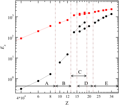
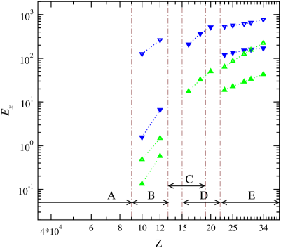
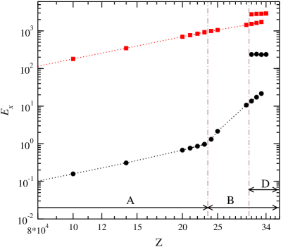
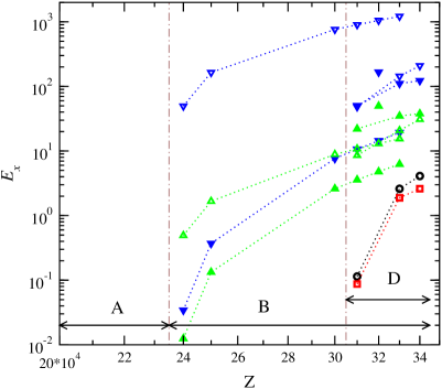
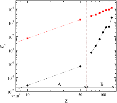
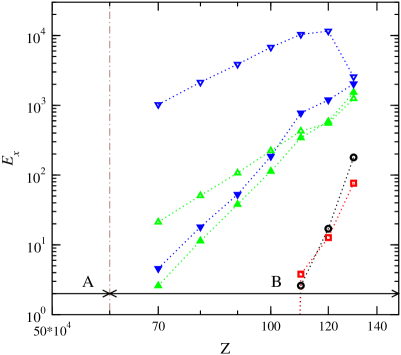
Figure 1: Time-averaged kinetic energy densities as functions of baroclinicity ${\mathrm{Z}}$ for parameter values (4) and $\mathrm{Pr}=0.05$, $\mathrm{Ek}=2/300$ (top two panels), $\mathrm{Pr}=0.05$, $\mathrm{Ek}=1/300$ (middle two panels), and $\mathrm{Pr}=0.03$, $\mathrm{Ek}=1/500$ (bottom two panels), Full and empty symbols indicate equatorially-symmetric and -asymmetric energy components, respectively. Black circles, red squares, green triangles-up and blue triangles-down indicate the energy components $\overline{E}_{p}^{s,a}$, $\overline{E}_{t}^{s,a}$, $\widetilde{E}_{p}^{s,a}$, $\widetilde{E}_{t}^{s,a}$, respectively. Axially-symmetric and axially-asymmetric components are plotted in the left and the right panels, respectively. Vertical dash-dotted lines indicate transition points. The ranges over which distinct states are observed are indicated by arrows near the bottom abscissa, with some states co-existing as indicated. Energy components not shown are at least 10 orders of magnitude smaller than the ones shown. (Colour online)

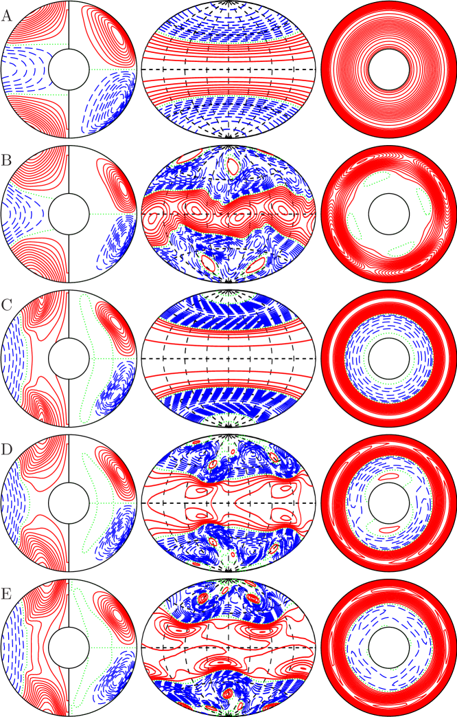
Figure 2: Flow structures with increasing baroclinicity ${\mathrm{Z}}\times 10^{-4}=1$, $12$, $18$, $18$ and $30$ from top to bottom for $\mathrm{Pr}=0.05$, $\mathrm{Ek}=2/300$ and fixed values (4). Bistability occurs at ${\mathrm{Z}}\times 10^{-4}=18$. The first plot in each row shows isocontours of $\overline{u}_{\varphi}$ (left half) and streamlines $r\sin\theta(\upartial_{\theta}\overline{v})=$ const. (right half) in the meridional plane. The second plot shows isocontours of $u_{r}$ at $r=r_{i}+0.7$ maped to the spherical surface using isotropic Aitoff projection. The third plot shows isocontours of $u_{r}$ in the equatorial plane. The isocontours are equidistant with positive isocontours shown by solid lines, negative isocontours shown by broken lines and the zeroth isocontour shown by a dotted line in each plot. All contour plots are snapshots at a fixed representative moment in time. Letters at each row denote corresponding flow states as indicated in Figure 1. (Colour online)

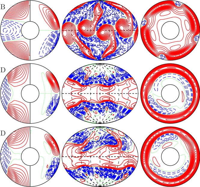
Figure 3: Flow structures with increasing baroclinicity ${\mathrm{Z}}\times 10^{-4}=30$, $32$, $34$ for $\mathrm{Pr}=0.05$, $\mathrm{Ek}=1/300$ and fixed values (4). The same quantities are plotted in each row as in Figure 2 and letters on the left side denote the corresponding flow state as in Figure 1. (Colour online)

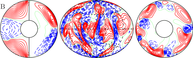
Figure 4: Flow in the case ${\mathrm{Z}}\times 10^{-4}=120$, for $\mathrm{Pr}=0.03$, $\mathrm{Ek}=1/500$ and fixed values (4). The same quantities are plotted in each row as in Figure 2 and letters denote the corresponding flow state as in Figure 1. (Colour online)

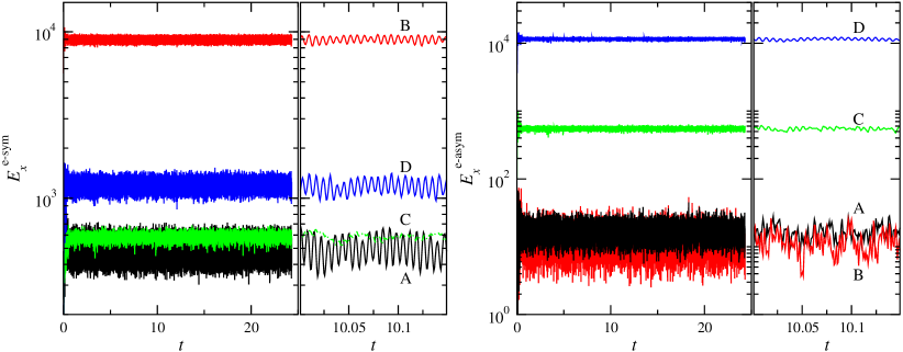
Figure 5: Time series of kinetic energy densities in the case shown in Figure 4. Equatorially symmetric components are shown in the left two panels and equatorially symmetric components are shown in the right two panels. The second panel in each group shows an enlarged segment of the time axis. The components $\overline{E}_{p}$, $\overline{E}_{t}$, $\widetilde{E}_{p}$, $\widetilde{E}_{t}$, are labelled in the plot and are also indicated by black lines, red lines, green lines and blue lines, respectively.

5 Instabilities of baroclinically-driven flows

The baroclinically-driven problem is invariant under a group of symmetry operations including rotations about the polar axis i.e. invariance with respect to the coordinate transformation $\varphi\to\varphi+\alpha$, reflections in the equatorial plane $\theta\to\pi-\theta$, and translations in time $t\to t+a$, see (Gubbins and Zhang 1993). As baroclinicity ${\mathrm{Z}}$ is increased the available symmetries of the solution are broken resulting in a sequence of states ranging from simpler and more symmetric flow patterns to more complex flow patterns of lesser symmetry. In this respect the system resembles Rayleigh-B´enard convection (Busse 2003).

Three sequences of non-magnetic simulations with gradually increasing values of the baroclinicity ${\mathrm{Z}}$ and fixed values of the other parameters were obtained and are shown in Figure 1. The first sequence is the most detailed one and allows us to capture the transitions that occur as the flow is more strongly driven while the other two sequences allow us to describe the effects of the variation in $\mathrm{Ek}$ and $\mathrm{Pr}$.

The sequence with $\mathrm{Pr}=0.05$ and $\mathrm{Ek}=2/300$ is illustrated in the top two panels of Figure 1 and in Figure 2. The sequence starts with the basic axisymmetric, equatorially symmetric and time-independent state with a dominant wave number $k=1$ in the radial direction labelled A in Figures 1 and 2. An instability occurs at about ${\mathrm{Z}}=9\times 10^{4}$ leading to a state B characterized by a dominant azimuthal wavenumber $m=2$ in the expansion of the solution in spherical harmonics $Y_{l}^{m}$, i.e. while the axisymmetry is broken, a symmetry holds with respect to the transformation $\varphi\to\varphi+\pi$. Simultaneously, the symmetry about the equatorial plane is also broken in state B. At ${\mathrm{Z}}=13\times 10^{4}$ a further transition to a pattern labelled C occurs. This state looks much like state A, i.e. it is axisymmetric, equatorially symmetric and time-independent but differs from state A in that it keeps a dominant radial wave number $k=2$. State C ceases to exists above $19\times 10^{4}$. At ${\mathrm{Z}}=22\times 10^{4}$ a further transition to a pattern labelled E occurs. State E seems to be related to state B in a way similar as state C is related to state B. Similarly to B, state E has a $m=2$ azimuthal symmetry and is asymmetric with respect to the equatorial plane. E differs from B, however, in that a dominant radial wave number $k=2$ develops. Remarkably, state C coexists with a pattern D that can be found for a range of values of ${\mathrm{Z}}$ from $15\times 10^{4}$ to $22\times 10^{4}$. Like C, state D is equatorially symmetric, has a dominant radial wave number $k=2$ and is time-independent. Unlike C it is not axisymmetric, but exhibits a $m=2$ structure. Which one of the coexisting patterns C and D will be found in a given numerical simulation depends on the initial conditions.

The Ekman number is decreased to $\mathrm{Ek}=1/300$ in our second sequence while we keep $\mathrm{Pr}=0.05$. The sequence is illustrated in the middle two panels of Figure 1 and in Figure 3. States C and E are not observed. State B becomes rather more pronounced with patches detaching from each other and with arms shooting towards the poles. State D loses its two-fold azimuthal symmetry $m=2$. In addition, state D becomes time-periodic at the largest values of ${\mathrm{Z}}$, e.g. at ${\mathrm{Z}}=34\times 10^{4}$ shown in the last row of Figure 3.

The Prandtl number is decreased to $\mathrm{Pr}=0.03$ and the Ekman number is further decreased to $\mathrm{Ek}=1/500$ in our third sequence. The kinetic energy components are plotted in the bottom two panels of Figure 1. In comparison with the preceding sequence, state D is not observed. For values of the baroclinicity larger than ${\mathrm{Z}}=110\times 10^{4}$ the spatial structure of state B becomes irregular as shown in Figure 4 and exhibits a chaotic time-dependence as illustrated by the time series of its kinetic energy components in Figure 5.

A summary of the symmetry properties of all distinct flow states identified is listed in Table 1 as is their capability of self-sustained dynamo action, see next section.

We wish to close this section by a brief comparison of baroclinically driven flows with the extensively studied problem of convective flows in rotating systems. Typical convection driven finite-amplitude instabilities are described for instance by (Sun et al. 1993, Simitev and Busse 2003, Busse and Simitev 2005b) and it is apparent that the baroclinically driven flows described in the article are essentially different. One feature that appears similar at first sight is the finding that baroclinically driven flows similarly to buoyancy-dominated convective turbulent flows (or equivalently slowly rotating convection) are characterised by retrograde (anti-solar) differential rotation. However, in rotating turbulent convection anti-solar rotation occurs after a sharp transition from prograde (solar) rotation as the buoyancy is gradually increased (Simitev et al. 2015), see also (Gastine et al. 2013, Käpylä et al. 2014). Moreover, convection in the solar rotation regime is characterised by elongated convective columns, known as “Busse columns”, while convection in the anti-solar regime is strongly disorganised, see (Simitev et al. 2015). Furthermore, anti-solar rotation is reversed to solar rotation in the presence of magnetic field (Simitev et al. 2015) and other effects of the magnetic field on this transition are reported in (Fan and Fang 2014, Karak et al. 2015). In contrast, in baroclinically driven flows anti-solar rotation occurs at all values of the baroclinicity starting from the basic flow state A, the baroclinic flow is regular and well-organised, and the magnetic fields generated by baroclinic dynamos do not reverse anti-solar rotation as seen in the figures of section 6 below.

	Equatorial	Azimuthal	Radial	Dynamo
	symmetry	symmetry	structure	capability
State A	yes	yes	1-roll	no
State B	no	2-fold	1-roll	yes
State C	yes	yes	2-roll	no
State D	yes	2-fold	2-roll	yes
State E	no	2-fold	2-roll	yes

Table 1: Summary of symmetry properties and dynamo capability of states in the case $\mathrm{Pr}=0.05$, $\mathrm{Ek}=2/300$ and fixed values (4).

6 Dynamos generated by baroclinically-driven flows

The possibility of dynamos generated in stably stratified stellar radiative regions has received only limited support in the literature, e.g. (Braithwaite 2006), because it is well known that dynamo action does not exist in a spherical system in the absence of a radial component of motion (Bullard and Gellman 1954, Kaiser and Busse 2017). The latter is, indeed, rather weak in the basic state A of low poloidal kinetic energy as discussed above. However, with increasing baroclinicity ${\mathrm{Z}}$, the growing radial component of the velocity field strengthens the likelihood of dynamo action. Indeed, the existence of dipolar dynamos sustained by the equatorially-symmetric flow state D was demonstrated in (Simitev and Busse 2017) for $\mathrm{Pr}=0.1$, $\mathrm{Ek}=2/300$ and $\mathrm{Pm}=16$. Below we investigate further the existence of dynamo action in all other baroclinically-driven flow states described in the preceding section.

A quadrupolar dynamo solution sustained by a baroclinically-driven flow in state B at $\mathrm{Pr}=0.03$, $\mathrm{Ek}=1/500$ and ${\mathrm{Z}}=100\times 10^{4}$ and for a magnetic Prandtl number value $\mathrm{Pm}=4$ is presented in Figure 6. This is a steady dynamo. The ratio of poloidal to toroidal magnetic energy is $E_{p}^{\text{magn}}/E_{t}^{\text{magn}}=0.033$, the ratio of $E^{\text{magn}}_{\text{dipole}}/E^{\text{magn}}_{\text{quadrupole}}=0.596$ and the ratio of magnetic to kinetic total energy is $E^{\text{magn}}/E^{\text{kin}}=0.009$. The magnetic field has a weaker dipolar component and a large-scale quadrupolar topology that does not change in time. The surface structure of the magnetic field is characterised by relatively strong inward magnetic flux at both poles. Four localised patches of inward magnetic flux appear in the equatorial region. The azimuthally-averaged toroidal field shows two large scale strong flux tubes near the pole. The azimuthally-averaged poloidal field is rather remarkable in that it remains almost completely confined to the spherical shell giving rise to an “invisible dynamo”.

This invisibility, however, does not persist as illustrated by a more strongly-driven quadrupolar dynamo at ${\mathrm{Z}}=110\times 10^{4}$ and $\mathrm{Pm}=2$ shown in Figure 7. The dynamo exhibits regular oscillations in which the quadrupole component reverses polarity.

B

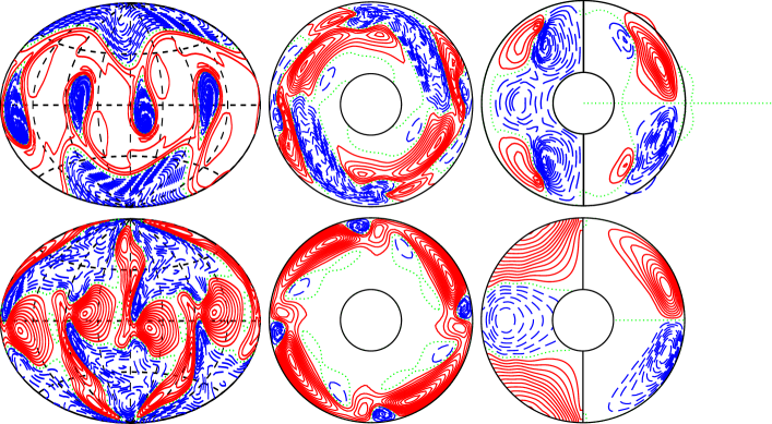
Figure 6: A dynamo solution for a flow in state B in the case ${\mathrm{Z}}\times 10^{-4}=100$, with $\mathrm{Pr}=0.03$, $\mathrm{Ek}=1/500$, $\mathrm{Pm}=4$ and values (4). First row: The first plot shows isocontours of radial magnetic field ${B}_{r}$ at $r=r_{o}+0.1$ in isotropic Aitoff projection. The second plot shows contours of $B_{r}$ in the equatorial plane. The third plot shows isocontours of $\overline{B}_{\varphi}$ (left half) and meridional field lines $r\sin\theta\,\upartial_{\theta}\overline{h}=$ const. (right half). Second row: The first plot shows isocontours of radial velocity $u_{r}$ at $r=r_{i}+0.7$ in isotropic Aitoff projection. The second plot shows contours of $u_{r}$ in the equatorial plane. The third plot shows isocontours of $\overline{u}_{\varphi}$ (left half) and streamlines $r\sin\theta(\upartial_{\theta}\overline{v})=$ const. (right half) in the meridional plane. All contour plots are snapshots at a fixed representative moment in time. The letter B denotes the corresponding flow state as indicated in Figure 1. (Colour online)

B

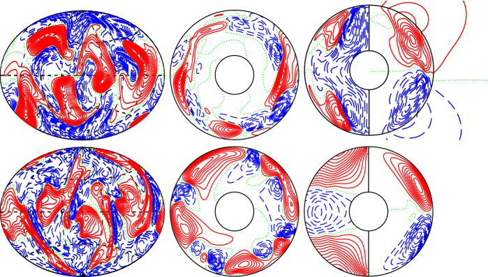
Figure 7: A dynamo solution for a flow in state B in the case ${\mathrm{Z}}\times 10^{-4}=110$, $\mathrm{Pr}=0.03$, $\mathrm{Ek}=1/500$, $\mathrm{Pm}=2$ and values (4). The same quantities are plotted as in Figure 6 and the letter B denotes the corresponding flow state as indicated in Figure 1. (Colour online)

D

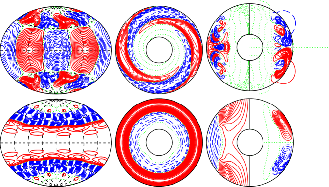
Figure 8: A dynamo solution for a flow in state D in the case ${\mathrm{Z}}\times 10^{-4}=32$, $\mathrm{Pr}=0.05$, $\mathrm{Ek}=1/300$, and $\mathrm{Pm}=5$ and values (4). The same quantities are plotted as in Figure 6 and the letter D denotes the corresponding flow state as indicated in Figure 1. (Colour online)

E

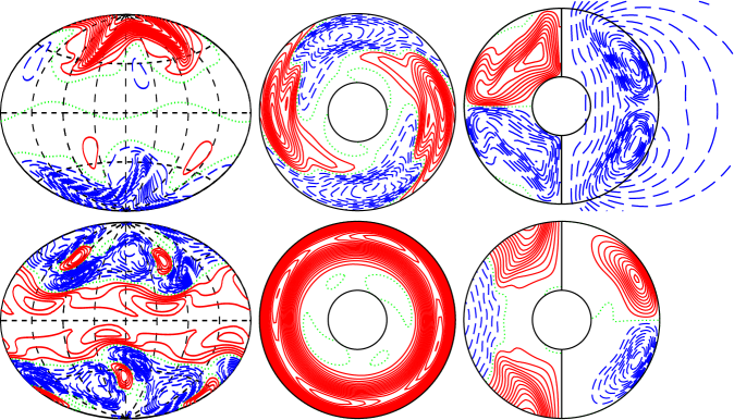
Figure 9: A dynamo solution for a flow in state E in the case ${\mathrm{Z}}\times 10^{-4}=34$, $\mathrm{Pr}=0.05$, $\mathrm{Ek}=2/300$, and $\mathrm{Pm}=1.5$ and values (4). The same quantities are plotted as in Figure 6 and the letter E denotes the corresponding flow state as indicated in Figure 1. (Colour online)

A multipolar dynamo solution sustained by a baroclinically-driven flow in state D at $\mathrm{Pr}=0.05$, $\mathrm{Ek}=1/300$ and ${\mathrm{Z}}=32\times 10^{4}$ and $\mathrm{Pm}=5$ is presented in Figure 8. This dynamo exhibits a steady time dependence. The ratio of poloidal to toroidal magnetic energy is $E_{p}^{\text{magn}}/E_{t}^{\text{magn}}=0.384$, the ratio of $E^{\text{magn}}_{\text{dipole}}/E^{\text{magn}}_{\text{quadrupole}}=0.0004$ and the ratio of magnetic to kinetic total energy is $E^{\text{magn}}/E^{\text{kin}}=0.003$. The spatial structure of the magnetic field of this dynamo is highly unusual in that it is not dominated by a large scale dipolar component ($Y_{1}^{0}$) or quadrupolar component ($Y_{2}^{0}$) as most other large scale dynamos reported to date but rather resembles approximately the structure of the $Y_{6}^{4}$ spherical harmonic function as seen in the leftmost plot in the upper row of Figure 8. Because of the weak $m=0$ contribution to the magnetic field the azimuthally-averaged components plotted in the rightmost plot in the upper row of Figure 8 are insignificant. It is remarkable that in this case the magnetic field significantly alters the fluid flow pattern as evident by comparison with the nonmagnetic simulation at identical parameter values shown in the second row of Figure 3, that was used as an initial condition for the dynamo run. The new magnetic flow pattern retains profiles of the differential rotation and the meridional circulation similar to those of the nonmagnetic case. However, the dominant azimuthal wave number increases from 2 to 4 with a stronger contribution of $m=0$. None of the other dynamos we report alter their generating flow states so significantly.

A dipolar dynamo generated by a baroclinically-driven flow in state E for $\mathrm{Pr}=0.05$, $\mathrm{Ek}=2/300$, ${\mathrm{Z}}\times=34\times 10^{4}$, and $\mathrm{Pm}=1.5$ is shown in Figure 9. The case has been started from an equilibrated neighbouring case to help convergence and reduce transients. The dynamo solution is steady. The ratio of poloidal to toroidal magnetic energy is $E_{p}^{\text{magn}}/E_{t}^{\text{magn}}=0.078$, the ratio of $E^{\text{magn}}_{\text{dipole}}/E^{\text{magn}}_{\text{quadrupole}}=5.97$ and the ratio of magnetic to kinetic total energy is $E^{\text{magn}}/E^{\text{kin}}=0.344$. Furthermore, the energy density of the magnetic field $E^{\text{magn}}$ is comparable to the kinetic energy density of the poloidal component of the velocity field, $E_{p}^{\text{kin}}$, with a ratio $E^{\text{magn}}/E_{p}^{\text{kin}}=1.42$. The magnetic field has a weaker quadrupolar component and a large-scale dipolar topology with prominent polar magnetic fluxes that does not change in time, as shown in Figure 9, resembling in this respect the surface fields of Ap-Bp stars (Donati and Landstreet 2009). The azimuthally-averaged toroidal field shows a pair of hook-shaped toroidal flux tubes largely filling each hemisphere of the shell. A large scale dipolar component emerges outside of the spherical shell. The structure of the fluid flow remains largely unaffected by the presence of the magnetic field.

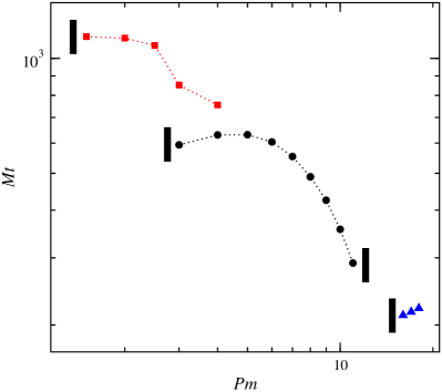
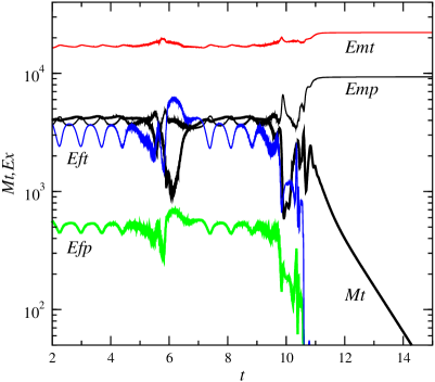
(a)	(b)

Figure 10: (Colour online) Left panel (a): Time-averaged total magnetic energy density as a function of the magnetic Prandtl number for $\mathrm{Ek}=2/300$ in the cases $\mathrm{Pr}=0.1$, ${\mathrm{Z}}=17\times 10^{4}$ (blue triangles), $Pr=0.08$, ${\mathrm{Z}}=20\times 10^{4}$ (black circles), $P=0.05$, ${\mathrm{Z}}=32\times 10^{4}$ (red squares). Small black rectangles indicate the boundary of a region of no dynamo excitation for the respective sequence. Right panel (b): Components of the magnetic and kinetic energy densities (as labelled) as a function of time in the case $Pr=0.08$, ${\mathrm{Z}}=20\times 10^{4}$, $\mathrm{Ek}=2/300$, $\mathrm{Pm}=12$.

An important issue for application of these results to astrophysical objects is to determine whether dynamo action persists at sufficiently small values of the magnetic Prandtl number. Figure 10(a) shows the dependence of the time-averaged total magnetic energy density on the magnetic Prandtl number for three sequences of self-sustained dynamo cases with $\mathrm{Ek}=2/300$. In each sequence no active dynamo is found for smaller values of $\mathrm{Pm}$; thus the smallest value of $\mathrm{Pm}$ is an estimate of the critical value of $\mathrm{Pm}$ for dynamo onset at fixed values of the other parameters. In particular, the figure shows that $\mathrm{Pm}_{\text{crit}}$ decreases as the value of the ordinary Prandtl number $\mathrm{Pr}$ is decreased and the value of the baroclinicity parameter ${\mathrm{Z}}$ is increased reducing $\mathrm{Pm}_{\text{crit}}$ to $1.5$ at $P=0.05$ and ${\mathrm{Z}}=32\times 10^{4}$. While it is numerically challenging to proceed in the direction of stronger baroclinic driving and smaller ordinary Prandtl number this trend, which we believe is likely to continue, indicates that baroclinically driven dynamos at more realistic values of $\mathrm{Pm}$ eventually exist. In this respect baroclinically driven dynamos seem to behave similarly to both Taylor-Couette dynamos (Willis and Barenghi 2002) and to randomly-forced small-scale dynamos (Schekochihin et al. 2004; 2005) where evidence is found that for fixed other parameter values a critical value of $Pm$ exists below which dynamo action is not possible. Surprisingly, Figure 10(a) also shows that there is an optimal value of $\mathrm{Pm}$ for magnetic field generation, e.g. $\mathrm{Pm}_{\text{opt}}=5$ at $\mathrm{Pr}=0.08$, ${\mathrm{Z}}=20\times 10^{4}$, and that dynamo action is lost when sufficiently large values of $\mathrm{Pm}$ are used. This appears to be due to a decline of the non-axisymmetric poloidal and toroidal kinetic energy components, $\widetilde{E}_{p}$ and $\widetilde{E}_{t}$, which are most strongly depleted by the magnetic field. This is related to the specific mechanism of dynamo excitation as discussed below.

A common feature of all dynamo-capable baroclinic flow states is that they exhibit significant non-axisymmetric flow components, $\widetilde{E}_{p}$ and $\widetilde{E}_{t}$ as seen in the left panels of Figure 1. These non-axisymmetric flow components appear to be essential for dynamo action as strikingly illustrated in Figure 10(b). Here a solution for $\mathrm{Pr}=0.08$, ${\mathrm{Z}}=20\times 10^{4}$, $\mathrm{Ek}=2/300$ and for $\mathrm{Pm}=12$ is shown. In the initial part of the simulation an oscillatory dipolar dynamo field is sustained by a flow in state D which is characterized by significant non-axisymmetric flow components. Flow state D, however, co-exists with flow state C which has negligibly small non-axisymmetric flow components and does not seem to support dynamo action. As $\widetilde{E}_{p}$ and $\widetilde{E}_{t}$ are weakened by the magnetic field a flow transition from state D to state C occurs after which the dynamo rapidly decays. On their own, the mean components of the flow which in the basic state A consist of radially-decreasing differential rotation (“subrotation”) coupled with counterclockwise meridional circulation in the northern hemisphere do not lead to dynamo excitation as also shown in kinematic dynamo models with prescribed laminar flows by Dudley and James (1989), see also (Latter and Ivers 2010). However, since the differential rotation remains the dominant flow component in all states the baroclinically driven dynamos reported here are of $\alpha\Omega$ type.

7 Conclusion

Evidence of dynamical processes such as differential rotation, meridional circulation, turbulence, and internal waves in radiative zones is emerging from helio- and asteroseismology (Turck-Chièze and Talon 2008, Thompson et al. 2003, Gizon et al. 2010, Chaplin and Miglio 2013, Aerts et al. 2010). These transport processes are important in the mixing of angular momentum as well as in the variation of chemical abundances (Miesch and Toomre 2009, Mathis 2013) and are thus critical for the formulation of a robust stellar evolution theory. Further, about 10% of observed main sequence and pre-main-sequence radiative stars exhibit detectable surface magnetic fields, (Donati and Landstreet 2009) posing the question of their origin. Thus, fluid motions in radiative zones and their dynamo capability are of significant interest.

Following our earlier work (Simitev and Busse 2017) we report additional direct numerical simulations of non-axisymmetric and time-dependent flows of anelastic fluids driven by baroclinic torques in stably stratified rotating spherical shells – a system serving as a simple model of a stellar radiative zone. We confirm that the general picture described in the latter study persists when values of the ordinary and the magnetic Prandtl number and of the Ekman number are changed up to a factor of 10. We find an additional baroclinic flow state E and we observe time-dependent behaviour in states B and D. The baroclinically driven flows appear very different from finite-amplitude convective flows in rotating systems as is apparent from comparisons with published results, e.g. (Sun et al. 1993, Grote et al. 2002, Simitev and Busse 2003). In particular, the retrograde differential rotation observed in the present baroclinic simulations does not seem to be related to the anti-solar rotation known to characterize turbulent convection in spherical shells rotating at slow rates (Simitev et al. 2015).

The increasing spatial and temporal complexity of baroclinic flow gives rise to the possibility of dynamo excitation. We have established that all baroclinically-driven flow states characterised by significant non-axisymmetric flow components, i.e. states labelled B, D and E, are capable of generating self-sustained magnetic fields for an appropriate range of values of the magnetic Prandtl number. Dynamo solutions with dipolar, quadrupolar and multipolar symmetries are found. These dynamos provide examples very different from the more familiar convection-driven dynamos (Busse and Simitev 2005a; b, Simitev and Busse 2012) and are certainly of general theoretical interest, e.g. some of them are sustained by essentially equatorially asymmetric flow fields. We have determined that a critical value of the magnetic Prandtl number for the onset of dynamo excitation $\mathrm{Pm}_{\text{crit}}$ exists similarly to Taylor-Couette dynamos (Willis and Barenghi 2002), randomly-forced small-scale turbulent dynamos (Schekochihin et al. 2004; 2005) and convectively-driven dynamos (Busse and Simitev 2005b) and within the range of our numerical simulations we find that $\mathrm{Pm}_{\text{crit}}$ decreases with the decrease of the ordinary Prandtl number and the increase of the baroclinicity parameter. A surprising new finding is that there exist an “upper” critical magnetic Prandtl number such that a shutdown of dynamo excitation and the decay of the magnetic field occurs at values in excess of it. This is due to a transition from a flow regime with significant non-axisymmetric components to a flow regime which is essentially axisymmetric caused by the presence of the magnetic field itself.

It must be admitted that our results are not likely to describe even semi-quantitatively the situation in any star. The choice of numerically accessible systems is too restricted for detailed comparisons with astrophysical observations. But we hope that various features described in this paper can eventually be related to observed magnetic properties of stars.

A baroclinic basic state is known to enhance the tidal instability in stellar equatorial planes (Kerswell 1993, Le Bars and Le Dizès 2006, Vidal et al. 2018). Thus baroclinically-driven flows could be even more capable of dynamo action and deserve further study. In terms of future work, it will be of interest to extend the present results to elliptic containers where tidal effects can be included. A further line of study is to investigate to what extent magnetic fields generated by baroclinic driving may be amplified by a tachocline shear layer at the top of the shell.

References

- Aerts et al. (2010) C. Aerts, J. Christensen-Dalsgaard, and D. Kurtz. Asteroseismology. Springer, 2010. 10.1007/978-1-4020-5803-5.
- Braginsky and Roberts (1995) S. Braginsky and P. Roberts. Equations governing convection in earth’s core and the geodynamo. Geophys. Astrophys. Fluid Dyn., 79(1-4):1–97, 1995. 10.1080/03091929508228992.
- Braithwaite (2006) J. Braithwaite. A differential rotation driven dynamo in a stably stratified star. Astron. & Astrophys., 449:451–460, 2006. 10.1051/0004-6361:20054241.
- Brandenburg and Subramanian (2005) A. Brandenburg and K. Subramanian. Astrophysical magnetic fields and nonlinear dynamo theory. Physics Reports, 417(1-4):1–209, oct 2005. 10.1016/j.physrep.2005.06.005.
- Bullard and Gellman (1954) E. Bullard and H. Gellman. Homogeneous dynamos and terrestrial magnetism. Phil. Trans. R. Soc. A, 247(928):213–278, 1954. 10.1098/rsta.1954.0018.
- Busse (1982) F. H. Busse. On the problem of stellar rotation. Astrophys. J., 259:759–766, 1982. 10.1086/160212.
- Busse (2003) F. H. Busse. The sequence-of-bifurcations approach towards understanding turbulent fluid flow. Surv. Geophys., 24(3):269–288, 2003. 10.1023/A:1024860722683.
- Busse and Simitev (2005a) F. H. Busse and R. D. Simitev. Convection in rotating spherical fluid shells and its dynamo states. In The Fluid Mechanics of Astrophysics and Geophysics. CRC Press, mar 2005a. 10.1201/9780203017692.ch12.
- Busse and Simitev (2005b) F. H. Busse and R. D. Simitev. Dynamos driven by convection in rotating spherical shells. Astronomische Nachrichten, 326(3-4):231–240, 2005b. ISSN 1521-3994. 10.1002/asna.200410382.
- Busse and Simitev (2011) F. H. Busse and R. D. Simitev. Remarks on some typical assumptions in dynamo theory. Geophys. Astrophys. Fluid Dyn., 105:234, 2011. 10.1080/03091929.2010.519891.
- Busse et al. (2003) F. H. Busse, E. Grote, and R. D. Simitev. Convection in rotating spherical shells and its dynamo action. In C. Jones, A. Soward, and K. Zhang, editors, Earth’s Core and Lower Mantle, pages 130–152. Taylor & Francis, London & New York, 2003. 10.1201/9780203207611.ch6.
- Chaplin and Miglio (2013) W. Chaplin and A. Miglio. Asteroseismology of solar-type and red-giant stars. Annu. Rev. Astron. Astrophys., 51(1):353–392, 2013. 10.1146/annurev-astro-082812-140938.
- Donati and Landstreet (2009) J.-F. Donati and J. Landstreet. Magnetic fields of nondegenerate stars. Annu. Rev. Astron. Astrophys., 47(1):333–370, 2009. 10.1146/annurev-astro-082708-101833.
- Dudley and James (1989) M. L. Dudley and R. W. James. Time-Dependent Kinematic Dynamos with Stationary Flows. Proceedings of the Royal Society A: Mathematical, Physical and Engineering Sciences, 425(1869):407–429, oct 1989. 10.1098/rspa.1989.0112.
- Espinosa and Rieutord (2013) L. Espinosa and M. Rieutord. Self-consistent 2d models of fast-rotating early-type stars. Astron. Astrophys., 552:A35, 2013. 10.1051/0004-6361/201220844.
- Fan and Fang (2014) Y. Fan and F. Fang. A simulation of convective dynamo in the solar convective envelope: Maintenance of the solar-like differential rotation and emerging flux. The Astrophysical Journal, 789(1):35, jun 2014. 10.1088/0004-637x/789/1/35.
- Gastine et al. (2013) T. Gastine, R. K. Yadav, J. Morin, A. Reiners, and J. Wicht. From solar-like to antisolar differential rotation in cool stars. Monthly Notices of the Royal Astronomical Society: Letters, 438(1):L76–L80, dec 2013. 10.1093/mnrasl/slt162.
- Gizon et al. (2010) L. Gizon, A. Birch, and H. Spruit. Local helioseismology: Three-dimensional imaging of the solar interior. Annu. Rev. Astron. Astrophys., 48(1):289–338, 2010. 10.1146/annurev-astro-082708-101722.
- Gough (1969) D. Gough. The anelastic approximation for thermal convection. J. Atmos. Sci., 26:448, 1969. 10.1175/1520-0469(1969)026¡0448:TAAFTC¿2.0.CO;2.
- Grote et al. (2002) E. Grote, F. H. Busse, and R. D. Simitev. Buoyancy Driven Convection in Rotating Spherical Shells and Its Dynamo Action. In High Performance Computing in Science and Engineering ’01, pages 12–34. Springer Berlin Heidelberg, 2002. 10.1007/978-3-642-56034-7_3.
- Gubbins and Zhang (1993) D. Gubbins and K. Zhang. Symmetry properties of the dynamo equations for palaeomagnetism and geomagnetism. Phys. Earth Planet. Inter., 75(4):225 – 241, 1993. 10.1016/0031-9201(93)90003-R.
- Hypolite and Rieutord (2014) D. Hypolite and M. Rieutord. Dynamics of the envelope of a rapidly rotating star or giant planet in gravitational contraction. Astron. Astrophys., 572:A15, 2014. 10.1051/0004-6361/201423378.
- Jones et al. (2011) C. Jones, P. Boronski, A. Brun, G. Glatzmaier, T. Gastine, M. Miesch, and J. Wicht. Anelastic convection-driven dynamo benchmarks. Icarus, 216(1):120 – 135, 2011. ISSN 0019-1035. 10.1016/j.icarus.2011.08.014.
- Kaiser and Busse (2017) R. Kaiser and F. H. Busse. On the robustness of the toroidal velocity theorem. Geophysical & Astrophysical Fluid Dynamics, 111(5):355–368, 2017. 10.1080/03091929.2017.1346634.
- Käpylä et al. (2014) P. J. Käpylä, M. J. Käpylä, and A. Brandenburg. Confirmation of bistable stellar differential rotation profiles. Astronomy & Astrophysics, 570:A43, oct 2014. 10.1051/0004-6361/201423412.
- Käpylä et al. (2017) P. J. Käpylä, M. J. Käpylä, N. Olspert, J. Warnecke, and A. Brandenburg. Convection-driven spherical shell dynamos at varying prandtl numbers. Astronomy & Astrophysics, 599:A4, 2017. 10.1051/0004-6361/201628973.
- Karak et al. (2015) B. B. Karak, P. J. Käpylä, M. J. Käpylä, A. Brandenburg, N. Olspert, and J. Pelt. Magnetically controlled stellar differential rotation near the transition from solar to anti-solar profiles. Astronomy & Astrophysics, 576:A26, mar 2015. 10.1051/0004-6361/201424521.
- Kerswell (1993) R. R. Kerswell. Elliptical instabilities of stratified, hydromagnetic waves. Geophysical & Astrophysical Fluid Dynamics, 71(1-4):105–143, 1993. 10.1080/03091929308203599.
- Lantz and Fan (1999) S. Lantz and Y. Fan. Anelastic magnetohydrodynamic equations for modeling solar and stellar convection zones. Astrophys. J. Suppl. Ser., 121(1):247, 1999. 10.1086/313187.
- Latter and Ivers (2010) H. Latter and D. Ivers. Spherical single-roll dynamos at large magnetic Reynolds numbers. Physics of Fluids, 22(6):066601, jun 2010. 10.1063/1.3453712.
- Le Bars and Le Dizès (2006) M. Le Bars and S. Le Dizès. Thermo-elliptical instability in a rotating cylindrical shell. Journal of Fluid Mechanics, 563:189, 2006. 10.1017/s0022112006001674.
- Marti et al. (2014) P. Marti, N. Schaeffer, R. Hollerbach, D. Cébron, C. Nore, F. Luddens, J.-L. Guermond, J. Aubert, S. Takehiro, Y. Sasaki, Y.-Y. Hayashi, R. D. Simitev, F. H. Busse, S. Vantieghem, and A. Jackson. Full sphere hydrodynamic and dynamo benchmarks. Geophys. J. Int., 197(1):119–134, 2014. 10.1093/gji/ggt518.
- Mathis (2013) S. Mathis. Transport processes in stellar interiors. In M. Goupil, K. Belkacem, C. Neiner, F. Lignières, and J. J. Green, editors, Studying Stellar Rotation and Convection: Theoretical Background and Seismic Diagnostics, pages 23–47. Springer, Berlin, Heidelberg, 2013. ISBN 978-3-642-33380-4. 10.1007/978-3-642-33380-4_2.
- Matsui et al. (2016) H. Matsui, E. Heien, J. Aubert, J. M. Aurnou, M. Avery, B. Brown, B. A. Buffett, F. H. Busse, U. R. Christensen, C. J. Davies, N. Featherstone, T. Gastine, G. A. Glatzmaier, D. Gubbins, J.-L. Guermond, Y.-Y. Hayashi, R. Hollerbach, L. J. Hwang, A. Jackson, C. A. Jones, W. Jiang, L. H. Kellogg, W. Kuang, M. Landeau, P. H. Marti, P. Olson, A. Ribeiro, Y. Sasaki, N. Schaeffer, R. D. Simitev, A. Sheyko, L. Silva, S. Stanley, F. Takahashi, S.-I. Takehiro, J. Wicht, and A. P. Willis. Performance benchmarks for a next generation numerical dynamo model. Geochem. Geophys. Geosys., 17(5):1586–1607, 2016. 10.1002/2015GC006159.
- Miesch and Toomre (2009) M. Miesch and J. Toomre. Turbulence, magnetism, and shear in stellar interiors. Annu. Rev. Fluid Mech., 41(1):317–345, 2009. 10.1146/annurev.fluid.010908.165215.
- Miesch et al. (2015) M. Miesch, W. Matthaeus, A. Brandenburg, A. Petrosyan, A. Pouquet, C. Cambon, F. Jenko, D. Uzdensky, J. Stone, S. Tobias, J. Toomre, and M. Velli. Large-eddy simulations of magnetohydrodynamic turbulence in heliophysics and astrophysics. Space Sci. Rev., 194(1):97–137, 2015. ISSN 1572-9672. 10.1007/s11214-015-0190-7.
- Rieutord (2006) M. Rieutord. The dynamics of the radiative envelope of rapidly rotating stars. Astron. Astrophys., 451(3):1025–1036, 2006. 10.1051/0004-6361:20054433.
- Rieutord and Beth (2014) M. Rieutord and A. Beth. Dynamics of the radiative envelope of rapidly rotating stars: Effects of spin-down driven by mass loss. Astron. Astrophys., 570:A42, 2014. 10.1051/0004-6361/201423386.
- Rieutord and Rincon (2010) M. Rieutord and F. Rincon. The Sun’s Supergranulation. Living Reviews in Solar Physics, 7, 2010. 10.12942/lrsp-2010-2.
- Schekochihin et al. (2004) A. A. Schekochihin, S. C. Cowley, J. L. Maron, and J. C. McWilliams. Critical Magnetic Prandtl Number for Small-Scale Dynamo. Physical Review Letters, 92(5), feb 2004. 10.1103/physrevlett.92.054502.
- Schekochihin et al. (2005) A. A. Schekochihin, N. E. L. Haugen, A. Brandenburg, S. C. Cowley, J. L. Maron, and J. C. McWilliams. The Onset of a Small-Scale Turbulent Dynamo at Low Magnetic Prandtl Numbers. The Astrophysical Journal, 625(2):L115–L118, may 2005. 10.1086/431214.
- Schwarzschild (1947) M. Schwarzschild. On stellar rotation. Astrophys. J., 106:427, 1947. 10.1086/144975.
- Simitev and Busse (2003) R. D. Simitev and F. H. Busse. Patterns of convection in rotating spherical shells. New J. Phys., 5:97, 2003. 10.1088/1367-2630/5/1/397.
- Simitev and Busse (2012) R. D. Simitev and F. H. Busse. Bistable attractors in a model of convection-driven spherical dynamos. Physica Scripta, 86(1):018409, 2012. 10.1088/0031-8949/86/01/018409.
- Simitev and Busse (2017) R. D. Simitev and F. H. Busse. Baroclinically-driven flows and dynamo action in rotating spherical fluid shells. Geophysical & Astrophysical Fluid Dynamics, 111(5):369–379, 2017. 10.1080/03091929.2017.1361945.
- Simitev et al. (2015) R. D. Simitev, A. Kosovichev, and F. H. Busse. Dynamo effects near the transition from solar to anti-solar differential rotation. Astrophys. J., 810(1):80, 2015. 10.1088/0004-637X/810/1/80.
- Spruit and Knobloch (1984) H. Spruit and E. Knobloch. Baroclinic instability in stars. Astron. Astrophys., 132:89–96, 1984.
- Sun et al. (1993) Z. Sun, G. Schubert, and G. Glatzmaier. Transitions to chaotic thermal convection in a rapidly rotating spherical fluid shell. Geophys. Astrophys. Fluid Dyn., 69(1):95–131, 1993. 10.1080/03091929308203576.
- Thompson et al. (2003) M. J. Thompson, J. Christensen-Dalsgaard, M. S. Miesch, and J. Toomre. The internal rotation of the sun. Annu. Rev. Astron. Astrophys., 41(1):599–643, 2003. 10.1146/annurev.astro.41.011802.094848.
- Tilgner (1999) A. Tilgner. Spectral methods for the simulation of incompressible flows in spherical shells. Int. J. Numer. Meth. Fluids, 30(6):713–724, 1999. 10.1002/(SICI)1097-0363(19990730)30:6%3C713::AID-FLD859%3E3.0.CO;2-Y.
- Turck-Chièze and Talon (2008) S. Turck-Chièze and S. Talon. The dynamics of the solar radiative zone. Adv. Space Res., 41(6):855–860, 2008. 10.1016/j.asr.2007.03.057.
- van Saders and Pinsonneault (2013) J. L. van Saders and M. H. Pinsonneault. Fast star, slow star; old star, young star: Subgiant rotation as a population and stellar physics diagnostic. The Astrophysical Journal, 776(2):67, sep 2013. 10.1088/0004-637x/776/2/67.
- Vidal et al. (2018) J. Vidal, D. Cébron, N. Schaeffer, and R. Hollerbach. Magnetic fields driven by tidal mixing in radiative stars. Monthly Notices of the Royal Astronomical Society, 475(4):4579–4594, 2018. 10.1093/mnras/sty080.
- von Zeipel (1924) H. von Zeipel. The radiative equilibrium of a rotating system of gaseous masses. Mon. Not. R. Astron. Soc., 84:665–683, 1924. 10.1093/mnras/84.9.665.
- Willis and Barenghi (2002) A. P. Willis and C. F. Barenghi. A Taylor-Couette dynamo. Astronomy & Astrophysics, 393(1):339–343, sep 2002. 10.1051/0004-6361:20021007.
- Zahn (1992) J.-P. Zahn. Circulation and turbulence in rotating stars. Astron. Astrophys., 265(1):115–132, 1992. URL http://adsabs.harvard.edu/abs/1992A%26A...265..115Z.