Adsorption of flexible polymer chains on a surface: Effects of different solvent conditions

Abstract

Polymer chains undergoing a continuous adsorption-desorption transition are studied through extensive computer simulations. A three-dimensional self-avoiding walk lattice model of a polymer chain grafted onto a surface has been treated for different solvent conditions. We have used an advanced contact-density chain-growth algorithm, in which the density of contacts can be directly obtained. From this quantity, the order parameter and its fourth-order Binder cumulant are computed, as well as the corresponding critical exponents and the adsorption-desorption transition temperature. As the number of configurations with a given number of surface contacts and monomer-monomer contacts is independent of the temperature and solvent conditions, it can be easily applied to get results for different solvent parameter values without the need of any extra simulations. In analogy to continuous magnetic phase transitions, finite-size-scaling methods have been employed. Quite good results for the critical properties and phase diagram of very long single polymer chains have been obtained by properly taking into account the effects of corrections to scaling. The study covers all solvent effects, going from the limit of super-self-avoiding walks, characterized by effective monomer-monomer repulsion, to poor solvent conditions that enable the formation of compact polymer structures.

I INTRODUCTION

The study of adsorption of polymer chains from a solution onto a flat solid surface has been extensively investigated for more than 60 years sinha , not only due to its relevance for potential technological and biological applications gennes ; milner ; meredith ; diaz ; bach14 , but also for its importance on many phenomena such as adhesion, surface coating, wetting, adsorption chromatography, among others (see, for example, Refs. bach14 ; fleer ). In the diluted regime, the chains can be considered independent of each other, and it is sufficient to investigate the surface effects on the conformations of a single polymer chain only. Such conformations, in their turn, can be determined by the temperature of the heat bath, the corresponding solvent quality, as well as the strengths of the monomer-monomer and monomer-surface interactions. In general, at sufficiently high temperatures and good solvent conditions, the polymer chain is expected to be extended and desorbed. However, at low temperatures, even a small attractive surface interaction is capable of keeping chain segments adsorbed bach14 ; eisen . As a result, a continuous adsorption-desorption (A-D) transition occurs at a critical temperature $T_{a}$, with a desorbed phase for $T>T_{a}$ and an adsorbed phase for $T<T_{a}$.

An appropriate order parameter for this A-D transition can be given by the ratio

$$n_{s}=N_{s}/N,$$ (1)

where $N_{s}$ is the number of monomers in contact with the surface and $N$ is the total length of the chain. It is clear that in the desorbed phase (for $T>T_{a}$), for very long chains, $n_{s}\rightarrow 0$. Thus, at the transition temperature $T_{a}$, a crossover exponent $\phi$ is defined for the behavior of the mean value of $N_{s}$ as a function of the chain length by eisen

$$\langle N_{s}\rangle\sim N^{\phi},~{}~{}\mbox{~{}~{}or}~{}~{}~{}~{}\langle n_{s}\rangle\sim N^{\phi-1},$$ (2)

which should be valid for long chains ($N\gg 1$).

In three dimensions, the precise value of this crossover exponent still remains an open question, even after decades of intensive research. For example, in the seminal work of Eisenriegler, Kremer, and Binder eisen on scaling relations for the adsorption transition, the estimated value was $\phi=0.58(2)$. Meirovitch and Livne meiro have used a scanning simulation method to obtain $\phi=0.530(7)$. On the other hand, Hegger and Grassberger hegger suggested that this exponent might be superuniversal, because they found $\phi=0.496(5)$, which is close to the exact result in two dimensions $\phi=0.5$. Another result towards the superuniversal character of this exponent has been reported by Metzger et al. metz ; metz2 , $\phi=0.50(2)$. According to Descas et al. descas , the determination of $\phi$ is strongly dependent on the estimation of the corresponding transition temperature $T_{a}$. In their work, both values $\phi=0.5$ and $\phi=0.59$ were considered acceptable, with the latter one being preferable. In a high-precision simulation using the pruned-enriched Rosenbluth method (PERM), Grassberger grass obtained $\phi=0.484(2)$. In agreement with this result, Klushin et al. binder estimated $\phi=0.483(3)$. Conversely, Luo luo reported a larger value, $\phi=0.54(1)$, while Taylor and Luettmer-Strathmann taylor , by means of Fisher partition function zeros, determined $\phi=0.515(25)$. In a previous paper we have obtained $\phi=0.492(4)$ pla and, very recently, Bradly et al. settled at $\phi=0.484(4)$ brad .

From what has been discussed above, one can clearly notice that the estimates of the crossover exponent cover a broad range and they are strongly dependent on the precise value of the critical temperature $T_{a}$. Additionally, the previous studies mostly consider good solvent conditions only, in which the monomer-monomer interaction has been neglected. It is, therefore, interesting to see whether the exponents (besides the crossover exponent $\phi$, there are critical exponents for other thermodynamic quantities, which will be defined below) vary or are universal as a function of the different solvent conditions, together with the construction of the corresponding phase diagram. Put in this way, a major contribution of the present work is the discussion of the dependence of the critical behavior and the critical exponents under all possible solvent conditions, which effectively extends the study to an entire class of hybrid polymer- adsorbent-solvent systems instead of a single-case scenario of good solvent conditions as has been done in the past.

In the present work, which is an extension of the recent results reported in reference pla , we treat the critical properties of the A-D transition of long chain polymers described by a coarse-grained model of self-avoiding random walk in three dimensions (i.e. chains with excluded volume interactions) with different solvent conditions by including an extra monomer-monomer interaction. In addition, we take advantage of the similarity of this geometrical transition with those in magnetic systems, and perform a finite-size scaling analysis luo ; puli . However, corrections-to-scaling effects will be considered in order to take into account the finiteness of the polymers length. It will be shown that the critical values are in fact in accord to some already discussed in the literature for good solvents, not only for the estimates of the transition temperature $T_{a}$ but also for the corresponding crossover exponent as well. For different values of the solvent conditions it is noted that the exponents vary and the presence of a multicritical point is expected along the phase transition line separating the adsorbed and desorbed phases.

The paper is organized as follows. In the next section the model is defined, while the computer simulational background is briefly described in section III. In section IV, we present details of the finite-size-scaling analysis and the results are discussed in section V. The last section contains additional comments and concluding remarks.

II self-avoiding ramdom walk MODEL on the simple cubic lattice

A simple and useful coarse-grained lattice polymer model for adsorption can be represented by an interacting self-avoiding random walk with additional monomer-substrate interaction. A polymer chain of length $N$ is formed by $N$ identical monomers occupying sites on a simple cubic lattice. Adjacent monomers in the polymer sequence have a fixed unitary bond length of one lattice unit. We consider a grafted polymer with one end covalently, and permanently, bound to the surface (i.e. it cannot desorb).

Each pair of nearest-neighbor non-bonded monomers possesses an energy $-\epsilon_{m}$. Thus, the key parameter for the energetic state of the polymer itself is the number of monomer-monomer contacts, $N_{m}$. The flat homogeneous and impenetrable substrate is located in the $z=0$ plane, and the polymer is restricted to $z>0$. All monomers lying in the $z=1$ plane are considered to be in contact with the substrate, and an energy $-\epsilon_{s}$ is attributed to each one of these surface contacts. Hence, the energetic contribution due to the interaction with the substrate is given by the number of surface contacts of the polymer, $N_{s}$.

The total energy of the model can then be written as bach05 ; bach14

$$E_{s}(N_{s},N_{m})=-\epsilon_{s}N_{s}-\epsilon_{m}N_{m}=-\epsilon_{s}(N_{s}+sN_{m}),$$ (3)

where $s=\epsilon_{m}/\epsilon_{s}$ is the ratio of the respective monomer-monomer and monomer-substrate energy scales. Actually, $s$ controls the solvent quality in such a way that larger $s$ values favor the formation of monomer-monomer contacts (poor solvent), whereas smaller values lead to a stronger binding to the substrate. For convenience, we set $\epsilon_{s}=1$ meaning that all energies are measured in units of the monomer-substrate interaction energy scale.

III SIMULATIONAL BACKGROUND

We used the contact-density chain-growth algorithm bach14 ; bach03 ; bach04 , where the density of contacts $g(N_{s},N_{m})$ is directly obtained from the simulation. This quantity represents the number of states for a given pair $N_{s}$ (number of contacts) and $N_{m}$ (monomer-monomer contacts). It does not depend on the temperature and the solvent parameter $s$. Thus, the temperature $T$ and the solubility parameter $s$ are external parameters that can be set after the simulation has finished.

We have simulated chains with lengths $N=16,~{}32,~{}64,~{}128,~{}256,~{}400,~{}\mbox{and}~{}503$ monomers. The total number of generated chains varied from $3.0\times 10^{8}$ for $N=16$ to $1.8\times 10^{9}$ for $N=503$. Statistical errors have been estimated by using the standard jackknife method quen . The $s$ values we considered here varied from $s=-10$ to $s=4$. It is noteworthy that other values of $s$ could be chosen without performing any extra simulations. However, since we already covered a significant region of the phase diagram, other values of solvent conditions would not provide any new qualitative insights into the transition behavior.

It is interesting to note that all relevant energetic thermodynamic observables can be obtained from the contact density $g(N_{s},N_{m})$. For instance, for a given pair $N_{s}$ and $N_{m}$, one can define the restricted partition function $Z_{T,s}^{r}(N_{s},N_{m})$ as

$$Z_{T,s}^{r}(N_{s},N_{m})=g(N_{s},N_{m})\exp[(N_{s}+sN_{m})/k_{B}T],$$ (4)

from which the canonical partition function is obtained as

$$Z_{T,s}=\sum_{N_{s},N_{m}}Z_{T,s}^{r}(N_{s},N_{m}).$$ (5)

Similarly, the mean value of any quantity $Q(N_{s},N_{m})$ can be computed from

$$\langle Q\rangle={{1}\over{Z_{T,s}}}\sum_{N_{s},N_{m}}Q(N_{s},N_{m})g(N_{s},N_{m})\exp\left[{{N_{s}+sN_{m}}\over{k_{B}T}}\right].$$ (6)

In the simulations we set $k_{B}=1$.

It is then clear that entropy, free energy, the average number of surface contacts $N_{s}$, the average number of monomer-monomer contacts $N_{m}$, heat capacity, cumulants, etc. are examples of functions that are easily calculable for any values of $T$ and $s$, as soon as $g(N_{s},N_{m})$ has been obtained from the simulations.

Now, in order to get the critical properties of the present model, instead of working with energetic quantities, such as the specific heat maximum kraw , which has been proven to have some pitfalls janse , or considering the scaling properties of the partition function grass ; binder , we will resort here to the scaling properties of the order parameter, and its derivatives, along the same lines as done in reference luo . However, we will take into account corrections to scaling and use convenient temperature derivatives of the order parameter $\langle n_{s}\rangle$, as well as scaling properties of the A-D transition temperature and the fourth-order cumulant of the order parameter.

So, from the simulations for each polymer length $N$, we can compute the mean value of the fraction of the number of monomer-substrate contacts, given by Eq. (1), and related quantities like the fourth-order cumulant

$$U_{4}(T)=1-\frac{\left<n_{s}^{4}\right>}{3\left<n_{s}^{2}\right>^{2}},$$ (7)

and the temperature derivative

$$\Gamma=-\frac{d\ln\langle n_{s}\rangle}{dT}.$$ (8)

IV Finite-size scaling (FSS) of the thermodynamic functions

IV.1 Magnetic systems

According to the finite-size scaling (FSS) theory for second-order phase transitions, it is well known that the singular part of the magnetic Gibbs free energy $G(t,h,L)$ of a finite magnetic system, close to its critical temperature, can be written as

$$G(t,h,L)=L^{-d}{\cal G}(L^{y_{t}}t,L^{y_{h}}h),$$ (9)

where $t=|T-T_{c}|/T_{c}$, $T_{c}$ being the infinite lattice critical temperature, $h$ is the external field, $L$ is the linear system size, and $d$ is the dimension of the lattice. The exponents in Eq. (9) are $y_{t}=1/\nu$ and $y_{h}=d-\beta/\nu$, where $\nu$ is the correlation length critical exponent and $\beta$ is the magnetization critical exponent. From the above relation, the scaling behavior of the magnetization, the specific heat, and the susceptibility can be obtained in a straightforward way.

From the free energy (9) and, for simplicity, considering zero external field $h=0$, it can be shown that any of the above specified quantities, generally designated by $P(t,L)$, scales as

$$P(t,L)=L^{\sigma/\nu}f_{P}(x),$$ (10)

where $\sigma$ is the critical exponent of $P$, namely $P(t,L\rightarrow\infty)=P_{0}t^{-\sigma}$ (with $P_{0}$ a non-universal constant) and $f_{P}(x)$ is a FSS function of $x=L^{1/\nu}t$. For instance, if $P$ is the magnetization one would have $\sigma=-\beta$. Similarly, one has $\sigma=\alpha$ and $\sigma=\gamma$ for the specific heat and susceptibility, respectively.

The FSS ansatz given by Eqs. (9) and (10) is valid only for sufficiently large systems and temperatures sufficiently close to the critical one. Corrections to scaling and finite-size scaling terms should appear for smaller systems and temperatures away from $T_{c}$, mainly due to irrelevant scaling fields and non-linear scaling fields. In general, such corrections can be implemented by generalizing (10) as

$$P(t,L)=L^{\sigma/\nu}f_{P}(x)\left[1+A_{P}(x)L^{-\omega}\right],$$ (11)

where $A_{P}(x)$ is another FSS function of $x=L^{1/\nu}t$ and $\omega$ is the corresponding leading order correction-to-scaling exponent.

IV.2 Adsorbed polymer chain

For the present coarse grained lattice polymer model for adsorption the natural size of the self-avoiding random walk chain is its length $N$. In analogy with magnetic systems, as given by Eq. (9), the polymer free energy should scale with temperature as

$$G(t,N)=N^{-1}{\cal G}(N^{1/\delta}t),$$ (12)

where we have now $y_{t}=1/\delta$ instead of $y_{t}=1/\nu$ in order to avoid confusion with Flory’s $\nu$ exponent widely used in polymer science.

The general scaling relation for the order parameter (2) reads

$$\langle n_{s}\rangle=N^{\phi-1}f_{n_{s}}(x)\left[1+A_{n_{s}}(x)N^{-\omega}\right],$$ (13)

where the above equation is a generalization of Eq. (2) by taking into account effects of corrections to scaling due to the finiteness of the polymer length and now $x=N^{1/\delta}(T-T_{a})$, $T_{a}$ being the adsorption critical temperature.

The corresponding fourth-order cumulant of the order parameter $U_{4}$ given by Eq. (7) (also known as Binder cumulant) should be independent of the chain length $N$ (for very long chains) bincum , and the maximum value of the quantity given by Eq. (8) is supposed to scale as

$${\Gamma}_{max}=-\left[{\frac{d\ln\langle n_{s}\rangle}{dT}}\right]_{max}=N^{1/\delta}f_{d}(x)\left[1+A_{d}(x)N^{-\omega}\right].$$ (14)

Accordingly, for the critical temperature one has the following scaling law, also based on continuous transitions in magnetic models,

$$T_{N}=T_{a}+N^{-1/\delta}f_{T}(x)\left[1+A_{T}(x)N^{-\omega}\right].$$ (15)

The exponent $\delta$ defined above is in fact the equivalent of the thermal critical exponent of the correlation length $\nu$ in ordinary magnetic continuous phase transitions. The functions $f_{i}(x)$, with $i=n_{s},~{}d,~{}T$, are FSS functions and $A_{i}(x)$ are non-universal functions (see, for instance, reference landaupa ).

Thus, the procedure we have to follow now is quite simple. From the simulations of each polymer size, we determine the exponent $1/\delta$ by using Eq. (14), which depends only on the maximum value of the derivative given by Eq. (8). In this case, we consider $f_{d}(x)$ and $A_{d}(x)$ as normal constants [we expect them not to vary much since the maximum positions should occur at temperatures close to the critical one so that one has $f_{d}(x=0)$ and $A_{d}(x=0)$]. With this exponent in hands, the critical temperature $T_{a}$ is obtained from Eq. (15) and, having the critical temperature, we are able to get the crossover exponent $\phi$ by using Eq. (13), where in this case we can also consider $x=0$.

V RESULTS

As a matter of comparison, and a test for the performance of the present approach, let us first discuss the corresponding results for the good solvent condition case $s=0$, where we have previous results originating from different methods.

V.1 Good solvent condition s=0

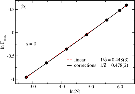
Figure 1: (color online) Results for $s=0$. (a) $\Gamma$, as defined in Eq. (8), as a function of temperature, for different polymer sizes. Smaller sizes have been omitted for clarity. (b) Logarithm of the maximum value of $\Gamma$ obtained in (a) as a function of the logarithm of the polymer length $N$ for different chain sizes. The dots correspond to the simulation results and the lines are the best fit according to Eq. (14), without corrections to scaling (linear, taking $A_{d}(x=0)=0$) and with corrections to scaling ($A_{d}(x=0)\neq 0$). The error bars are smaller than the symbol sizes.

Fig. 1 shows results obtained by using Eqs. (8) and (14). In Fig. 1(a) we have plotted $\Gamma$ as a function of temperature for several polymer lengths. The corresponding logarithm of its maximum value as a function of the logarithm of the polymer length $N$ for different chain sizes is shown in Fig. 1(b). From the linear fit one gets $1/\delta=0.448(3)$, while taking into account corrections to scaling one gets $1/\delta=0.478(2)$. Although the corresponding data are rather close, as can be seen in Fig. 1(b), the value of the $1/\delta$ exponent is sensitive when one considers correction to scaling. This value should be compared to the estimate $1/\delta=0.56$ from reference luo and $1/\delta=0.485(6)$ from reference brad , where the latter ones have been obtained from different procedures.

The fourth-order Binder cumulant, as a function of the temperature, is shown in Fig. 2. One can clearly see that there is a systematic crossing of the larger chains with relation to the smallest one ($N=16$). Taking these crossings as $T_{N}$, for $N\geq 32$, we can plot them as a function of $N^{-1/\delta}$, where $1/\delta$ has been computed from the data of Fig. 1. The corresponding results are depicted in Fig. 3. We note that corrections to scaling are more important in this case and the value $T_{a}=3.494(2)$, so calculated, is comparable to the values $T_{a}=3.500(1)$ obtained by Klushin et al. binder , $T_{a}=3.44(2)$ by Luo luo , and the most recent estimate $T_{a}=3.520(6)$ obtained by Bradly et al. brad . All these estimates were obtained by different approaches.

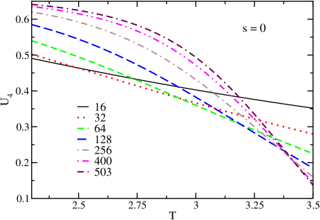
Figure 2: (color online) Fourth-order Binder cumulant $U_{4}$ as a function of the temperature $T$ for different chain sizes for $s=0$.

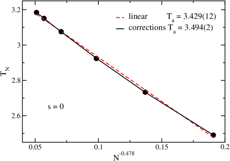
Figure 3: (color online) Transition temperature $T_{N}$ as a function of $N^{-1/\delta}$ for $s=0$. The dots correspond to the crossings of the fourth-order Binder cumulant for chain lengths $N\geq 32$ with the result for $N=16$, as shown in Fig. 2. The lines are the best fit according to Eq. (15), without corrections to scaling (linear, taking $A_{T}(x=0)=0$) and with corrections to scaling ($A_{T}(x=0)\neq 0$).

Once the critical temperature has been calculated, one can now utilize the scaling relation (13) to get the crossover exponent. The results are shown in Fig. 4. Although not visible in the scale of the figure, the corrections to scaling are important in this case as well, and the computed value $\phi=0.492(4)$ is also in agreement with the result quoted in reference brad , $\phi=0.485(6)$, and quite close to the value $\phi=0.483(2)$ given in reference binder (these results are smaller than the estimate $0.56$ obtained by Luo luo ).

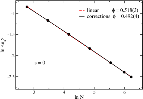
Figure 4: (color online)Logarithm of the order parameter $\langle n_{s}\rangle$ as a function of the logarithm of the polymer length $N$ for different chain sizes, for $s=0$, at the transition temperature $T_{a}$. The dots correspond to the simulation results and the lines are the best fit according to Eq. (13), without corrections to scaling (linear, taking $A_{n_{s}}(x=0)=0$) and with corrections to scaling ($A_{n_{s}}(x=0)\neq 0$).

From the above results, we can see that the present approach can furnish quite good results for the special case $s=0$, when compared to the values previously obtained from other procedures. The corresponding values of the critical behavior are displayed in Table 1, together with those from references  binder , luo , and brad for a comparison. However, our approach has the advantage of being easily extended to get the critical behavior for other values of the solvent condition parameter $s$ without any extra simulation.

Table 1: Adsorption critical temperature $T_{a}$ and crossover exponents $\phi$ and $1/\delta$ for some selected values of the solvent conditions $s$. For comparison, some values for $s=0$ coming from different methods are also shown. The last row gives the estimate of the correction-to-scaling exponent.

$s$	$T_{a}$	$\phi$	1/$\delta$
-10	3.31(1)	0.469(5)	0.44(1)
-5	3.303(4)	0.473(3)	0.448(1)
-2	3.358(4)	0.478(3)	0.450(8)
-1	3.407(3)	0.482(3)	0.453(8)
0	3.494(2)	0.492(4)	0.478(2)
0binder	3.500(1)	0.483(2)	–
0luo	3.44(2)	0.54(1)	0.56
0brad	3.520(6)	0.484(4)	=$\phi$
1	3.788(9)	0.524(4)	0.59(3)
1.5	4.60(2)	0.353(4)	0.52(1)
2	5.74(2)	0.228(2)	0.39(1)
2.5	6.87(7)	0.20(3)	0.29(1)
3	7.9(1)	0.205(2)	0.232(7)
		$\omega=0.5(1)$

V.2 Different solvent conditions $s\neq 0$

The behavior of the thermodynamic quantities for other values of the solvent conditions are qualitatively similar to those presented in Figs. 1-4. For example, the behavior of $\Gamma$ as a function of temperature is shown for different polymer chains for $s=-2$ in Fig. 5(a) and for $s=2$ in Fig. 5(b). The logarithm of the maximum value of $\Gamma$, as a function of the logarithm of the polymer length $N$, for the different chain sizes, is shown in Fig. 6 for both values of solvent conditions, together with the previous data of good solvent for comparison. The values of the exponent $1/\delta$ include corrections to scaling.

Fig. 7 depicts the behavior of the fourth-order Binder cumulant for $s=-2$ [Figure 7(a)] and $s=2$ [Figure 7(b)]. From these curves the crossings of the cumulants with the smaller chain ($N=16$) can be determined in order to compute $T_{N}$ for $N\geq 32$ under each solvent condition. The corresponding results are presented in Fig. 8 together with the respective fits and extrapolated adsorbed critical temperature $T_{a}$. The previously obtained value of the adsorbed transition temperature for $s=0$ is also included in Fig. 8 for comparison. We note that the scale of the curves for $s=-2$ and $s=0$ are the same, showing that there is not a sensitive variation in $T_{a}$ as for $s=2$.

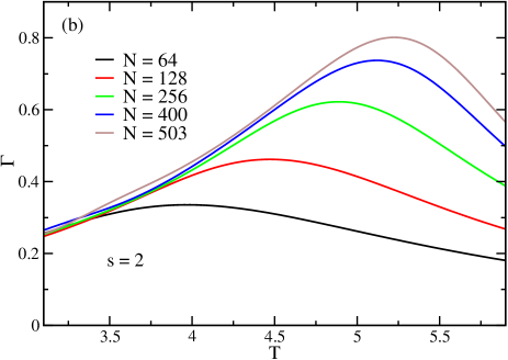
Figure 5: (color online) $\Gamma$, as defined in Eq. (8), as a function of temperature, for different polymer sizes. In (a) we have $s=-2$ and in (b) $s=2$. In both cases, smaller sizes have been omitted for clarity.

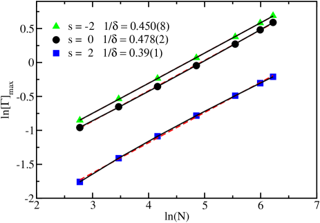
Figure 6: (color online) Logarithm of the maximum value of $\Gamma$ obtained from the data of Fig. 5, as a function of the logarithm of the polymer length $N$, for different chain sizes. The dots correspond to the simulation results and the lines are the best fit according to Eq. (14). Dashed lines without corrections to scaling (linear, taking $A_{d}(x=0)=0$) and full lines with corrections to scaling ($A_{d}(x=0)\neq 0$). Only the values coming from correction to scaling are listed in the figure. The error bars from the simulations are smaller than the symbol sizes.

With the values of $T_{a}$ we can proceed and compute the crossover exponent $\phi$. The results are shown in Fig. 9. In all the fits one can notice that corrections to scaling are indeed important in obtaining the critical behavior of the polymer. For easier comparison, all results are compiled in Table 1, together with some additional selected values for different solvent conditions $s$.

V.3 Discussion of the phase diagram and critical behavior

Although the scaling behavior of the thermodynamic quantities for general solvent conditions ($s\neq 0$) is qualitatively similar to that for good solvent ($s=0$) the character of the adsorption transition changes considerably. This is clearly seen in the phase diagram shown in Fig. 10. Results for $s=0$ from Refs. binder , luo , and brad , also included in this figure, fit very well into the extended picture of polymer adsorption presented here. For poor solvent ($s>0$), desorbed and adsorbed polymer conformations are much more compact. The self-interacting polymer undergoes a collapse and an additional freezing transition, and both transitions compete with the adsorption transition, depending on the solvent conditions. From the estimates for transition temperatures and critical exponents, we find that the specific parametrization of the critical behavior depends in fact on the solvent quality. As Table 1 shows, the values of the exponents obtained for $s\neq 0$ are significantly different. Obviously, the solvent quality has a noticeable quantitative influence on the adsorption behavior.

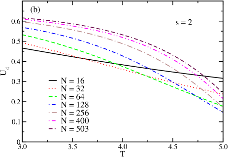
Figure 7: (color online) Fourth-order Binder cumulant $U_{4}$ as a function of the temperature $T$ for different chain sizes for (a) $s=-2$ and (b) $s=2$.

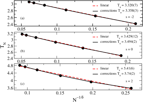
Figure 8: (color online) Transition temperature $T_{N}$ as a function of $N^{-1/\delta}$ for $s=-2$ (a), $s=0$ (b), and $s=2$ (c). The values of the exponents $1/\delta$, for each solvent condition, come from the data of Fig. 6. The dots correspond to the crossings of the fourth-order Binder cumulant for chain lengths $N\geq 32$ with the result for $N=16$, as shown in Figs. 2 and 7. The lines are the best fit according to Eq. (15). Dashed lines without corrections to scaling (linear, taking $A_{T}(x=0)=0$) and full lines with corrections to scaling ($A_{T}(x=0)\neq 0$).

Figure 9: (color online) Logarithm of the order parameter $\langle n_{s}\rangle$ as a function of the logarithm of the polymer length N, for different chain sizes, at the transition temperature $T_{a}$, obtained from Fig. 8. The dots correspond to the simulation results and the lines are the best fit according to Eq. (15). Dashed lines without corrections to scaling (linear, taking $A_{d}(x=0)=0$) and full lines with corrections to scaling ($A_{d}(x=0)\neq 0$). Only the values coming from correction to scaling are listed in the figure. The error bars from the simulations are smaller than the symbol sizes.

On the other hand, if $s$ is negative, the monomer-monomer interaction is repulsive, and the polymer avoids forming nearest-neighbor contacts. This mimics the effect of a good solvent. In the limit $s\rightarrow-\infty$, the system is represented by what we may call a “super-self-avoiding walk” (SSAW) model, where the contacts between nearest neighbors are forbidden. This effectively increases the excluded volume and the corresponding adsorption temperature of the system is expected to be smaller than for $s=0$. To our knowledge, this case has not yet been studied and there are no values to compare with. However, as our results suggest, the corresponding critical adsorption temperature of this intrinsically non-energetic SSAW should be $T_{a}\lesssim 3.31$.

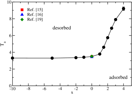
Figure 10: Critical temperature $T_{a}$ as a function of $s$ for the adsorbed-desorbed transition. Results for $s=0$ from references binder ; luo ; brad are also shown for comparison. The line is just a guide to the eyes.

Increasing the value of $s$ effectively increases the conformational entropy at a given energy in the phase of adsorbed conformations more than in the desorbed phase. As a consequence, the slope of the microcanonical entropy (or the density of states) becomes smaller near the transition point, which, in turn, results in a larger adsorption temperature. The phase diagram plotted in Fig. 10 shows exactly this behavior for the adsorption temperature.

For all $s$ values, the adsorption transition is of second-order. Figure 11 depicts the behavior of the exponents $\phi$ and $1/\delta$ if the solvent quality $s$ is changed. We find that their values vary along the second-order transition line, meaning that this transition seems to be non-universal. Moreover, they cross each other close to $s=0$ and both exponents exhibit a peak near $s\sim 1.5$. These peaks can be an indication of the presence of a multicritical point in this region bell ; vrb ; raj ; owc . In fact, various additional crossovers between different adsorbed phases in the high-$s$ regime are expected. Analyses for a finite system puli2 show a complex structure of adsorbed compact phases in this regime, but simulations of sufficiently large systems which would allow for a thorough finite-size scaling analysis are extremely challenging. Therefore, the discussion of the nature of separate tricritical points or a single tetracritical point with coil-globule transition lines extending into the desorbed and the adsorbed phases and the crystallization behavior near the adsorption line should be left as a future work.

Finally, something should be said about the correction-to-scaling exponent $\omega$. In all of the fits, we have noted that it did not change significantly as we changed the parameter $s$, in contrast to $\phi$ and $1/\delta$. In addition, the fits are not sensitive upon variation of $\omega$. Thus, all of our results have been obtained using an exponent $\omega=0.5(1)$.

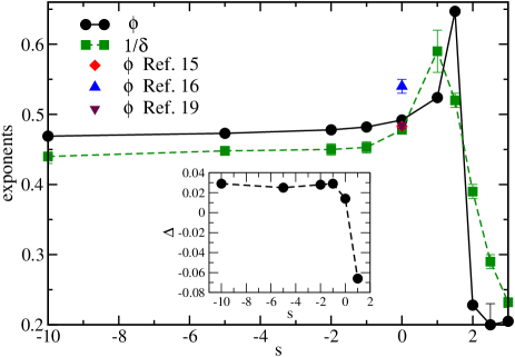
Figure 11: (color online) Critical exponents $\phi$ and $1/\delta$ as a function of the solvent parameter $s$. Results for $s=0$ from references binder ; luo ; brad are also shown for comparison. The lines are guides to the eyes only. The inset shows the difference between the exponets $\Delta=\phi-1/\delta$ as a function of $s$.

VI Additional Comments and Concluding Remarks

The adsorption/desorption transition of long polymers grafted on a surface has been studied in simulations employing the contact-density chain-growth algorithm, where the density of contacts is directly obtained. This quantity can be used to analyze the thermodynamic behavior for any value of temperature and solvent conditions. By using finite-size scaling theory, taking into account properly the corrections to scaling, we constructed the phase diagram in the temperature versus solvent parameter space and estimated the critical exponents. Our results are comparable to estimates found in the literature for good solvent condition ($s=0$). In particular, they agree very well with those reported by Klushin et al. binder , obtained by a different approach. On the other hand, the agreement with the results from Luo luo is less satisfactory. Although Luo has used a similar FSS for some quantities, the present work has considered an additional scaling relation [given by Eq. (14)] and resorted to corrections to scaling. The present values are also quite comparable to the more recent ones obtained by Bradly et al. brad , who have likewise included corrections to scaling in their fits.

The phase diagram and the critical exponents suggest that the critical line is not universal. Moreover, the exponents present a peak near the region $s\sim 1.5$, indicating the existence of a possible multicritical point. The presence of this multicritical point can be associated to the existence of different conformational phases of the polymer in the adsorbed phase, with first-order transitions between them. At least one of these first-order transition lines will end up at the multicritical point. However, whether or not there is only one first-order line or several lines, is not clear at the moment. In addition, the rather strong variation of the critical exponents, as well as the corresponding critical temperature near this region, can be the cause of the difficulty encountered in getting the criticality of the model, even for $s=0$. Naturally, more simulations in the ordered adsorbed region should be very welcome to precisely determine the behavior of the transition lines close to the multicritical point.

We have also estimated the adsorbed transition temperature $T_{a}$ from the position of the maximum values of $\Gamma$, as depicted in Figs. 1(a) and 5. However, this quantity turned out to be less robust than the fourth-order Binder cumulant $U_{4}$ and seems to have similar pitfalls like the specific heat based measurement kraw .

Regarding the critical exponents $\phi$ and $1/\delta$, it is apparent from the scaling theory that they are independent exponents, as has been reported by Klushin et al. binder . However, in the recent work by Bradly et al. brad , it has been shown that, although independent, $\phi$ and $1/\delta$ have the same value, at least for $s=0$. Indeed, with an argument similar to that used in Ref. brad , one can show that they are identical for $s=0$. For instance, close to the adsorbing transition temperature the free energy of the polymer chain can be given by Eq. (12). On the other hand, the energy, U, is given by

$$U={{\partial\left(\beta G\right)}\over{\partial\beta}}=-{{1}\over{k_{B}T^{2}}}{{\partial\left(\beta G\right)}\over{\partial T}},$$ (16)

where $\beta=1/k_{B}T$. Close to the transition temperature $T_{a}$, $\beta G=\beta_{a}G$ where $\beta_{a}=1/k_{B}T_{a}$, leading to

$$U=-k_{B}{\beta_{a}}^{3}N^{1/\delta-1}{\cal G}^{\prime}(x),$$ (17)

where ${\cal G}^{\prime}(x)$ is the derivative of ${\cal G}(x)$ with respect to $x$. Nonetheless, for $s=0$, one also has from Eq. (3)

$$U={{\langle E_{s}\rangle}\over{N}}=-\epsilon\langle n_{s}\rangle=-\epsilon_{s}N^{\phi-1}f_{ns}(x).$$ (18)

From the above equations one concludes that $\phi=1/\delta$.

We can see from Table 1 that the values of $\phi$ and $1/\delta$ are not equal, but close taking into account the numerical error. We would also like to emphasize that it is far more efficient to directly simulate self-avoiding walks instead of interacting self-avoiding walks, as has been done here with sophisticated algorithmic efforts. In particular, simpler methodologies would enable simulations of much longer chains for the case $s=0$, and in this case a better test for the equality of $\phi$ and $1/\delta$ would be achieved. However, we believe that the polymer lengths we have considered in this paper are sufficiently long to allow for the quantitative discussion of the adsorption transition for all solvent conditions.

The above argument, however, holds only for $s=0$, where the internal energy and the order parameter are related. Such relation does not hold as soon as $s\neq 0$. The behavior of the critical exponents $\phi$ and $1/\delta$, as a function of $s$, depicted in Fig. 11 clearly shows that despite being different for general solvent conditions, they do meet at $s=0$. The inset in Fig. 11 shows the difference of the critical exponents $\Delta=\phi-1/\delta$ as a function of the solvent conditions. Assuming their equality at $s=0$, from the data of Table 1 we estimate $\phi=1/\delta=0.485(7)$, in quite good agreement with $\phi=1/\delta=0.484(4)$ from Ref. brad .

Another important issue raised in Ref. brad concerns the universality of this system. The present results indicate a non-universal behavior as a function of $s$, while Bradly et al. claim that the critical exponents should be universal. They reached this conclusion by studying the self-avoiding trail in the cubic lattice, which presented the same critical exponents as the self-avoiding walk. However, the self-avoiding trail does not seem to correspond to any value of $s$ in our simulations. It would be, however, desirable to simulate the self-avoiding trail with monomer-monomer interactions in order to see whether the corresponding exponents will differ or not from the good solvent condition.

We believe that it is still premature to decisively claim non-universal behavior with different values for both exponents. In order to seek for a universal behavior we could, in addition of present analysis, consider the same exponent $1/\delta$ along the $s$ line and determine the corresponding transition temperature $T_{a}$ with this exponent, as shown in Figs. 3 and 8. However, in doing so, a different $T_{a}$ is obtained with the corresponding critical exponent $\phi$ not only diferent from $1/\delta$ but also $s$ dependent.

Still within the scope of universality, since the exponents should be equal for $s=0$, such behavior seems to violate both universality and weak universality hypotheses (as is well known, in the weak universality the exponents vary but their ratio is constant). This kind of violation of both hypothesis has been recently reported for the ferromagnetic phase transition of (Sm_1-yNd_y)_0.52Sr_0.48MnO₃ single crystals with ($0.5\leq y\leq 1$), where the magnetic exponents vary with Nd concentration $y$ khan . Our polymer adsorption model can be seen as a similar example of such new scaling behavior, providing also a generic route leading to continuous variation of critical exponents and multi-criticality. In fact, one of the open major problems is the precise identification of multicritical points and their physical understanding. This study requires an in-depth treatment of the different structural phases of the polymer and the corresponding transition lines between them in the adsorbed and desorbed phases, which is far from being easy. Whereas there has been a history of progress, none of the existing results can be considered conclusive. The most recent approach to use a generalized microcanonical statistical analysis method reveals a multitude of features whose explanation requires additional careful analyses. This discussion, however, is beyond the scope of this manuscript and will be published once the analysis of the structural transitions has been completed.

VII ACKNOWLEDGMENTS

The authors would like to thank Prof. Thomas Prellberg for stimulating discussions. This work has been supported partially by CNPq (Conselho Nacional de Desenvolvimento Científico e Tecnológico, Brazil) under Grant No. 402091/2012-4 and by the NSF under Grant No. DMR-1463241. PHLM also acknowledges FAPEMAT (Fundação de Amparo à Pesquisa do Estado de Mato Grosso) for the support (Grant No. 219575/2015).

References

- (1) R. Sinha, H. L. Frisch, and F. R. Eirich, J. Chem. Phys. 57, 584 (1953).
- (2) P. G. de Gennes, Macromolecules 13, 1069 (1980).
- (3) S. T. Milner, Science 251, 905 (1991).
- (4) J. C. Meredith and K. P. Johnston, Macromolecules 31, 5518 (1998).
- (5) M. F. Diaz, S. E. Barbosa, and N. J. Capiati, Polymer 48, 1058 (2007).
- (6) M. Bachmann, Thermodynamics and Statistical Mechanics of Macromolecular Systems (Cambridge University Press, Cambridge, 2014).
- (7) G. J. Fleer, M. A. Cohen Stuart, J. M. H. M. Scheutjens, T. Cosgrove, and B. Vincent, Polymers at Interfaces (Chapman & Hall, London, 1993).
- (8) E. Eisenriegler, K. Kremer, and K. Binder, J. Chem. Phys. 77, 6296 (1982).
- (9) H. Meirovitch and S. Livne, J. Chem. Phys. 88, 4507 (1998).
- (10) R. Hegger and P. Grassberger, J. Phys. A: Math. Gen. 27, 4069 (1994).
- (11) S. Metzger, M. Müller, K. Binder, and J. Baschnagel, J. Chem. Phys. 118, 8489 (2003).
- (12) S. Metzger, M. Müller, K. Binder, and J. Baschnagel, Macromol. Theory Simul. 11, 985 (2002).
- (13) R. Descas, J.-U. Sommer, and A. Blumen, J. Chem. Phys. 120, 8831 (2004).
- (14) P. Grassberger, J. Phys. A: Math. Gen. 38, 323 (2005).
- (15) L. I. Klushin, A. A. Polotsky, H-P Hsu, D. A. Markelov, K. Binder, and A. M. Skvortsov, Phys. Rev. E 87, 022604 (2013).
- (16) M-B Luo, J. Chem. Phys. 128, 044912 (2008).
- (17) M. P. Taylor and J. Luettmer-Strathmann, J. Chem. Phys. 141, 204906 (2014).
- (18) J. A. Plascak, P. H. L. Martins, and M. Bachmann, Phys. Rev. E 95, 050501(R) (2017).
- (19) C. J. Bradly, A. L. Owczarek, and T. Prellberg, Phys. Rev. E 97 022503 (2018).
- (20) P. H. L. Martins and M. Bachmann, Physics Procedia 68 90 (2015)
- (21) M. Bachmann and W. Janke, Phys. Rev. Lett. 95, 058102 (2005).
- (22) M. Bachmann and W. Janke, Phys. Rev. Lett. 91 208105 (2003).
- (23) M. Bachmann and W. Janke, J. Chem. Phys. 120 6779 (2004).
- (24) M. H. Quanouille, Ann. Math. Statist. 20, 355 (1949).
- (25) J. Krawczyk, I. Jensen, A. L. Owczarek, and S. Kumar, Phys. Rev. E 79, 031912 (2009).
- (26) E. J. Janse van Rensburg and A. R. Rechnitzer, J. Phys. A: Math. Gen. 37, 6875 (2004).
- (27) K. Binder, Z. Physik B 43, 119 (1981).
- (28) D. P. Landau, Physica A 205, 41 (1994).
- (29) K. De’Bell and T. Lookman, Rev. Mod. Phys. 65, 87 (1993).
- (30) T. Vrbová and S. G. Whittington, J. Phys. A: Math. Gen. 31, 3989 (1998).
- (31) R. Rajesh, D. Dhar, D. Giri, S. Kumar, and Y. Singh, Phys. Rev. E 65, 056124 (2002).
- (32) A. L. Owczarek, A. Rechnitzer, J. Krawczyk, and T. Prellberg, J. Phys. A: Math. Gen. 40, 13257 (2007).
- (33) P. H. L. Martins and M. Bachmann, Phys. Chem. Chem. Phys. 18, 2143 (2016).
- (34) N. Khan, P. Sarkar, A. Midya, P. Mandal, and P.K. Mohanty, Sci. Rep. 7 45004 (2017).