Elastic Functional Principal Component Regression

Abstract

We study regression using functional predictors in situations where these functions contain both phase and amplitude variability. In other words, the functions are misaligned due to errors in time measurements, and these errors can significantly degrade both model estimation and prediction performance. The current techniques either ignore the phase variability, or handle it via pre-processing, i.e., use an off-the-shelf technique for functional alignment and phase removal. We develop a functional principal component regression model which has comprehensive approach in handling phase and amplitude variability. The model utilizes a mathematical representation of the data known as the square-root slope function. These functions preserve the $\mathbb{L}^{2}$ norm under warping and are ideally suited for simultaneous estimation of regression and warping parameters. Using both simulated and real-world data sets, we demonstrate our approach and evaluate its prediction performance relative to current models. In addition, we propose an extension to functional logistic and multinomial logistic regression

Keywords: Compositional noise, functional data analysis, functional Principal Component Analysis, functional regression

1 Introduction

The statistical analysis of functional data is fast gaining prominence in the statistics community because “big data” is central to many applications. For instance, functional data can be found in a broad swath of application areas ranging from biology, medicine, and chemistry; to geology, sports, and financial analysis. In this problem, some of the random quantities of interest are functions of independent variables, (e.g., time, frequency), and are studied as elements of an appropriate function space, often a Hilbert space. The analysis can include common statistical procedures such as computing statistical summaries, estimating parametric and nonparametric distributions, and generating inferences under noisy observations. One common problem in functional data analysis is regression modeling where the function variables are used as predictors to estimate a scalar response variable.

More precisely, let the predictor functions be given by $\{f_{i}:[0,T]\rightarrow,~{}~{}i=1,2,\dots,n\}$ and the corresponding response variables be $y_{i}$. The standard functional linear regression model for this set of observations is

$$y_{i}=\alpha+\int_{0}^{T}f_{i}(t)\beta(t)\,dt+\epsilon_{i},~{}~{}i=1,\dots,n$$ (1.1)

where $\alpha\in$ is the intercept, $\beta(t)$ is the regression-coefficient function and $\epsilon_{i}\in$ are random errors. This model was first studied by Ramsay and Dalzell (1991) and Cardot et al. (1999). The model parameters are usually estimated by minimizing the sum of squared errors (SSE),

$$\{\alpha^{*},\beta^{*}(t)\}=\operatorname*{arg\,min}_{\alpha,\beta(t)}\sum_{i=1}^{n}|y_{i}-\alpha-\int_{0}^{T}f_{i}(t)\beta(t)\,dt|^{2}.$$

These values form maximum-likelihood estimators of parameters under the additive white-Gaussian noise model. One problem with this approach is the solution is an element of an infinite-dimensional space while its specification for any $n$ is finite dimensional; resulting in an infinite number of possible solutions without further restrictions imposed on the problem. Ramsay and Silverman (2005) proposed two approaches to handle this issue: (1) Represent $\beta(t)$ using $p$ basis functions in which $p$ is kept large to allow desired variations of $\beta(t)$, and (2) add a roughness penalty term to the objective function (SSE) which selects a smooth solution by finding an optimal balance between the SSE and the roughness penalty. The basis can come from Fourier analysis, splines, or functional PCA (Reiss and Ogden (2007)).

Current literature in functional linear regression is focused primarily on the estimation of the coefficient of $\beta(t)$ under a basis representation. For example, (Cuevas et al., 2002; Cardot et al., 2003; Hall and Horowitz, 2007; James et al., 2009) discuss estimation and/or inference of $\beta(t)$ for different cases for the standard functional linear model and the interpretation of $\beta(t)$. Focusing on prediction of the scalar response, Cai and Hall (2006) studied the estimation of $\int f_{i}(t)\beta(t)\,dt$. In some situations the response variable $y_{i}$, is categorical and the standard linear model will not suffice. James (2002) extended the standard functional linear model to functional logistic regression to be able to handle such situations. Müller and Stadtmüller (2005) extended the generalized model to contain a dimension reduction by using a truncated Karhunen-Loève expansion. Recently, Gertheiss et al. (2013) included variable selection to reduce the number of parameters in the generalized model.

In practice the predictor functions are observed at discrete points and not the full interval $[0,T]$. Furthermore, in some situations, these observations are corrupted by noise along the time axis. That is, one observes $\{(t+\eta(t),f(t))\}$ instead of $\{(t,f(t))\}$ where the random variables $\eta(t)$ are constrained so that the observation times do not cross each other. While some papers have assumed parametric models for $\eta(t)$ (Carroll et al. (2006)) and incorporated them in the estimation process, the others have ignored them completely. It is more natural to treat these measurement variables in a nonparametric form as follows: We assume that observation times are given by $\gamma(t)$ where $\gamma$ is a monotonic function with appropriate boundary conditions ($\gamma(0)=0,\ \gamma(T)=T$). Consequently, the observations are modeled as $\{\gamma(t),f(t)\}$ where $\gamma$ captures a random noise component that needs to be accounted for in the estimation process. The effect of $\gamma$ is a warping of $f$, with a nonlinear shift in the locations of peaks and valleys but no changes in the heights of those peaks and valleys. In this effect warping differs across realizations (observations) and, hence, is termed as warping or compositional noise. Some authors have also called it the phase variability in functional data. If the phase variability is ignored, the resulting model may fail to capture patterns present in the data and will lead to inefficient data models. One way to handle this noise is to capture both the phase and amplitude variability properly in the regression model. It is more natural to include handling of warping noise, or alignment, in the regression model estimation itself; and perform a joint inference on all model variables under the same objective function. Recently, Gervini (2015) has proposed a functional linear regression model that includes phase-variability in the model. This uses a random-effect simultaneous linear model on the warping parameters and the principal component scores (of aligned predictor functions). However, this method involves PCA on the original functional space and has shown to be inferior for unaligned data (Tucker et al. (2013):Lee and Jung (2017)). Tucker et al. (2013) showed that if this variability is not accounted for properly when performing fPCA, the results will be misleading due to incorrect shape of the calculated mean function.

In this paper we focus on problems where the functional data contains random phase variability. To handle that variability, we propose a regression model that incorporates the phase variability through the use of functional principal component regression (fPCR); where this variability is handled in a harmonious way. The basic idea is to use a PCA method as the basis that is able to capture the amplitude variability, phase variability, or both in the regression problem. This allows the model to capture the variability that is important in predicting the outcome from the data. Using this representation and the geometry of the warping function $\gamma$, we construct the model and outline the resulting prediction procedures. The fPCR method was first proposed by Reiss and Ogden (2007), but they neglected to account for the phase-variability found in functional data. We extend this framework to the logistic regression case where the response can take on categorical data. We will illustrate this application using both simulated and real data sets, which includes sonar, gait, and electrocardiogram data. The physiological data is studied in the context of classification of disease types or the separation of individuals.

This paper is organized as follows: In Section 2 we review the relevant material from functional regression, and in Section 3 we develop the elastic functional PCR model. In Section 4 we extend the elastic fPCR to the logistic and multinomial logistic case. In Sections 5 and 6, we report the results of applying the proposed approach to a simulated data set and seven real data sets from various application domains. Finally, we close with a brief summary and some ideas for future work in Section 7.

2 Functional Principal Component Regression

We start with a more common functional regression model, and then develop an “elastic” principal component version that accounts for phase variability of the functional data. Without loss of generality we assume the time interval of interest to be $[0,1]$. Let $f$ be a real-valued function on $[0,1]$; from a theoretical perspective we restrict to functions that are absolutely continuous on $[0,1]$ and we let ${\mathcal{F}}$ denote the set of all such functions. In practice, since observed data are discrete, this assumption is not a restriction.

2.1 Functional Principal Component Regression Model

Let $\{f_{i}\}$ denote observations of a predictor function variable and let $y_{i}\in$, be the corresponding response variable. The standard functional linear regression model for this set of observations is

$$y_{i}=\alpha+\int f_{i}(t)\beta(t)\,dt+\epsilon_{i},~{}~{}i=1,\dots,n$$ (2.1)

where $\alpha$ is the bias and $\beta(t)$ is the regression coefficient function. The model is usually determined by minimizing the sum of squared errors (SSE).

$$\{\alpha^{*},\beta^{*}(t)\}=\operatorname*{arg\,min}_{\alpha,\beta(t)}\sum_{i=1}^{n}|y_{i}-\alpha-\int f_{i}(t)\beta(t)\,dt|^{2}.$$ (2.2)

One problem with this approach, is that for any finite $n$, it is possible to perfectly interpolate the responses if no restrictions were are placed on $\beta(t)$. Specifically, since $\beta(t)$ is infinite dimensional, we have infinite degrees of freedom to form $\beta(t)$ in which we can make the SSE equal zero. Ramsay and Silverman (2005) proposed two approaches with the first, representing $\beta(t)$ using a $p$-dimensional basis in which $p$ is hopefully large enough to capture all variations of $\beta(t)$. The second approach is adding a penalty term which shrinks the variability of $\beta(t)$ or smooths its response.

Functional principal component regression uses the principal components as the basis functions where the model is determined by minimizing

$$\{\alpha^{*},\mathbf{b}^{*}\}=\operatorname*{arg\,min}_{\alpha,\mathbf{b}}\sum_{i=1}^{n}|y_{i}-\alpha-\sum_{j=1}^{n_{o}}\left\langle f_{i}(t),\xi_{j}(t)\right\rangle b_{j}|^{2},$$ (2.3)

where $n_{o}$ principal components are used, $\xi(t)$ is the corresponding eigenfunction, and $\mathbf{b}=[b_{1},\dots,b_{j}]$. It should be noted that $f_{i}(t)$ here is mean centered.

3 Elastic Functional Principal Component Regression Model

In order to properly account for the variability, we can use the vertical fPCA and horizontal fPCA presented in Tucker et al. (2013). These PCA methods account for the variability, by first separating the phase and amplitude and then performing the PCA on the spaces separately. Using these methods, one can construct a regression on the amplitude space using the square-root slope function (SRSF), $q$ and specifically the aligned SRSF or the phase space using the warping functions, $\gamma$, the motivation for the using of SRSF will be explained later. A third option is to use the method developed by Lee and Jung (2017) which is an extension of the method developed by Tucker et al. Lee proposes a combined fPCA which generates a function $g^{C}$, which combines the function ($f$) and the warping function. We propose a slight modification to this work to use the SRSF, due to its theoretical properties. The combined function does work on a simplified geometry of the warping function where the warping function, is transformed to the Hilbert Sphere; and the shooting vector that maps to the tangent space is analyzed. This simplification, and SRSF modification allows the use of a metric that is a proper distance as in the vertical and horizontal case. By using the combined fPCA the regression model can be performed on the amplitude and phase simultaneously. Table 1 presents the three domains and where the regression is performed.

Table 1: Functional Principal Component Regression Domains.

	Vertical fPCA	Horizontal fPCA	Combined fPCA
Domain	$\tilde{q}$	$\gamma$	$g^{C}=[\tilde{q}~{}~{}Cv(t)]$
Variability	Amplitude	Phase	Amplitude + Phase
Metric	Fisher-Rao	Fisher-Rao	Fisher-Rao

3.1 Elastic Functional fPCA

We begin by giving a short review of the vertical and horizontal fPCA of Tucker et al. (2013) and the combined phase-amplitude fPCA method of Lee and Jung (2017), with a slight modification which will be described clearly in later sections. These methods are based on the functional data analysis approach outlined in Srivastava et al. (2011), Kurtek et al. (2011), and Tucker et al. (2013); see those references for more details on this background material.

Let $\Gamma$ be the set of orientation-preserving diffeomorphisms of the unit interval $[0,1]$: $\Gamma=\{\gamma:[0,1]\rightarrow[0,1]|~{}\gamma(0)=0,~{}\gamma(1)=1,\gamma~{}\text{is a diffeomorphism}\}$. Elements of $\Gamma$ play the role of warping functions. For any $f\in{\mathcal{F}}$ and $\gamma\in\Gamma$, the composition $f\circ\gamma$ denotes the time-warping of $f$ by $\gamma$. With the composition operation, the set $\Gamma$ is a Lie group with the identity element $\gamma_{id}(t)=t$. This is an important observation since the group structure of $\Gamma$ is seldom utilized in past papers on functional data analysis.

As described in Tucker et al. (2013), there are two metrics to measure the amplitude and phase variability of functions. These metrics are proper distances, one on the quotient space ${\mathcal{F}}/\Gamma$ (i.e., amplitude) and the other on the group $\Gamma$ (i.e., phase). The amplitude or $y$-distance for any two functions $f_{1},\ f_{2}\in{\mathcal{F}}$ is defined as

$$d_{a}(f_{1},f_{2})=\inf_{\gamma\in\Gamma}\|q_{1}-(q_{2}\circ\gamma)\sqrt{\dot{\gamma}}\|,$$ (3.1)

where $q(t)=\mbox{sign}(\dot{f}(t))\sqrt{|\dot{f}(t)|}$ is known as the square-root slope function (SRSF) ($\dot{f}$ represents the derivative of $f$). The optimization problem in Equation 3.1 is most commonly solved using a Dynamic Programming algorithm; see Robinson (2012) for a detailed description. If $f$ is absolutely continuous, then $q\in\mathbb{L}^{2}([0,1],)$ (Robinson (2012)), henceforth denoted by $\mathbb{L}^{2}$. For the properties of the SRSF and the reason for its use in this setting, we refer the reader to Srivastava et al. (2011), Marron et al. (2015) and Lahiri et al. (2015). Moreover, it can be shown that for any $\gamma_{1},\gamma_{2}\in\Gamma$, we have $d_{a}(f_{1}\circ\gamma_{1},f_{2}\circ\gamma_{2})=d_{a}(f_{1},f_{2})$, i.e., the amplitude distance is invariant to function warping.

3.2 Simplifying Geometry of $\Gamma$

The space of warping functions, $\Gamma$, is an infinite-dimensional nonlinear manifold, and therefore cannot be treated as a standard Hilbert space. To overcome this problem, we will use tools from differential geometry to perform statistical analyses and to model the warping functions. The following framework was previously used in various settings including; (1) modeling re-parameterizations of curves (Srivastava and Jermyn (2009)), (2) putting prior distributions on warping functions (Kurtek (2017) and Lu et al. (2017)), (3) studying execution rates of human activities in videos (Veeraraghavan et al. (2009)), and many others. It is also very closely related to the square-root representation of probability density functions introduced by Bhattacharya (1943), and later used for various statistical tasks (see e.g., Kurtek and Bharath (2015)).

We represent an element $\gamma\in\Gamma$ by the square-root of its derivative $\psi=\sqrt{\dot{\gamma}}$. Note that this is the same as the SRSF defined earlier, and takes this form since $\dot{\gamma}>0$. The identity $\gamma_{id}$ maps to a constant function with value $\psi_{id}(t)=1$. Since $\gamma(0)=0$, the mapping from $\gamma$ to $\psi$ is a bijection, and one can reconstruct $\gamma$ from $\psi$ using $\gamma(t)=\int_{0}^{t}\psi(s)^{2}ds$. An important advantage of this transformation is that since $\|\psi\|^{2}=\int_{0}^{1}\psi(t)^{2}dt=\int_{0}^{1}\dot{\gamma}(t)dt=\gamma(1)-\gamma(0)=1$, the set of all such $\psi$s is the positive orthant of the Hilbert sphere $\Psi=\mathbb{S}_{\infty}^{+}$ (i.e., a unit sphere in the Hilbert space $\mathbb{L}^{2}$). In other words, the square-root representation simplifies the complicated geometry of $\Gamma$ to a unit sphere. The distance between any two warping functions, i.e., the phase distance, is exactly the arc-length between their corresponding SRSFs on the unit sphere $\mathbb{S}_{\infty}$:

$$d_{p}(\gamma_{1},\gamma_{2})=d_{\psi}(\psi_{1},\psi_{2})\equiv\cos^{-1}\left(\int_{0}^{1}\psi_{1}(t)\psi_{2}(t)dt\right)\ .$$

Figure 1 shows an illustration of the SRSF space of warping functions as a unit sphere.

Figure 1: Depiction of the SRSF space of warping functions as a sphere and a tangent space at the identity element $\psi_{id}$.

3.3 Mapping to the Tangent Space at Identity Element

While the geometry of $\Psi\subset\mathbb{S}_{\infty}$ is more tractable, it is still a nonlinear manifold and computing standard statistics remains difficult. Instead, we use a tangent (vector) space at a certain fixed point for further analysis. The tangent space at any point $\psi\in\Psi$ is given by: $T_{\psi}(\Psi)=\{v\in\mathbb{L}^{2}|\int_{0}^{1}v(t)\psi(t)dt=0\}$. To map between the representation space $\Psi$ and tangent spaces, one requires the exponential and inverse-exponential mappings. The exponential map at a point $\psi\in\Psi$ denoted by $\exp_{\psi}:T_{\psi}(\Psi)\mapsto\Psi$, is defined as

$$\exp_{\psi}(v)=\cos(\|v\|)\psi+\sin(\|v\|)\frac{v}{\|v\|},$$ (3.2)

where $v\in T_{\psi}(\Psi)$. Thus, $\exp_{\psi}(v)$ maps points from the tangent space at $\psi$ to the representation space $\Psi$. Similarly, the inverse-exponential map, denoted by $\exp_{\psi}^{-1}:\Psi\mapsto T_{\psi}(\Psi)$, is defined as

$$\exp_{\psi}^{-1}(\psi_{1})=\frac{\theta}{\sin(\theta)}(\psi_{1}-\cos(\theta)\psi),$$ (3.3)

where $\theta=d_{p}(\gamma_{1},\gamma)$. This mapping takes points from the representation space to the tangent space at $\psi$.

The tangent space representation $v$ is sometimes referred to as a shooting vector, as depicted in Figure 1. The remaining question is which tangent space should be used to represent the warping functions. A sensible point on $\Psi$ to define the tangent space is the sample Karcher mean $\hat{\mu}_{\psi}$ (corresponding to $\hat{\mu}_{\gamma}$) of the given warping functions or the identity element $\psi_{id}$. For details on the definition of the sample Karcher mean and how to compute it, please refer to Tucker et al. (2013).

3.4 Vertical Functional Principal Components

Let $f_{1},\cdots,f_{n}$ be a given set of functions, and $q_{1},\cdots,q_{n}$ be the corresponding SRSFs, ${\mu}_{q}$ be their Karcher Mean, and let $\tilde{q}_{i}$s be the corresponding aligned SRSFs using Algorithm 1 from Tucker et al. (2013). In performing vertical fPCA, one needs to include the variability associated with the initial values, i.e., $\{f_{i}(0)\}$, of the given functions. Since representing functions by their SRSFs ignores this initial value, this variable is treated separately. That is, a functional variable $f$ is analyzed using the pair $(q,f(0))$ rather than just $q$. This way, the mapping from the function space $\mathcal{F}$ to $\mathbb{L}^{2}\times$ is a bijection. In practice, where $q$ is represented using a finite partition of $[0,1]$, say with cardinality $T$, the combined vector $h_{i}=[q_{i}~{}~{}f_{i}(0)]$ simply has dimension $(T+1)$ for fPCA. We can define a sample covariance operator for the aligned combined vector $\tilde{h}=[\tilde{q}_{1}~{}~{}f_{i}(0)]$ as

$$K_{h}=\frac{1}{n-1}\sum_{i=1}^{n}E[(\tilde{h}_{i}-\mu_{h})(\tilde{h}_{i}-\mu_{h})^{\mathsf{T}}]\in\mathbb{R}^{(T+1)\times(T+1)}\ ,$$

where $\mu_{h}=[\mu_{q}~{}~{}\bar{f}(0)]$. Taking the SVD, $K_{h}=U_{h}\Sigma_{h}V_{h}^{\mathsf{T}}$ we can calculate the directions of principle variability in the given SRSFs using the first $p\leq n$ columns of $U_{h}$ and can be converted back to the function space $\mathcal{F}$, via integration, for finding the principal components of the original functional data. Moreover, we can calculate the observed principal coefficients as $\left\langle\tilde{h}_{i},U_{h,j}\right\rangle$.

One can then use this framework to visualize the vertical principal-geodesic paths. The basic idea is to compute a few points along geodesic path $\tau\mapsto\mu_{h}+\tau\sqrt{\Sigma_{h,jj}}U_{h,j}$ for $\tau\in$ in $\mathbb{L}^{2}$, where $\Sigma_{h,jj}$ and $U_{h,j}$ are the $j^{th}$ singular value and column, respectively. Then, obtain principle paths in the function space $\mathcal{F}$ by integration.

3.5 Horizontal Functional Principal Components

To perform horizontal fPCA we will use the tangent space at $\mu_{\psi}$ to perform analysis, where $\mu_{\psi}$ is the mean of the transformed warping functions. Algorithm 2 from Tucker et al. (2013) can be used to calculate this mean. In this tangent space we can define a sample covariance function:

$$K_{\psi}=\frac{1}{n-1}\sum_{i=1}^{n}E[v_{i}v_{i}^{\mathsf{T}}]\in^{T\times T}.$$

The singular value decomposition (SVD) of $K_{\psi}=U_{\psi}\Sigma_{\psi}V_{\psi}^{\mathsf{T}}$ provides the estimated principal components of $\{\psi_{i}\}$: the principal directions $U_{\psi,j}$ and the observed principal coefficients $\left\langle v_{i},U_{\psi,j}\right\rangle$. This analysis on $\mathbb{S}_{\infty}$ is similar to the ideas presented in Srivastava et al. (2005) although one can also use the idea of principal nested sphere for this analysis Jung et al. (2012). The columns of $U_{\psi}$ can then be used to visualize the principal geodesic paths.

3.6 Combined Functional Principal Components

To model the association between the amplitude of a function and its phase, Lee and Jung (2017) use a combined function $g^{C}$ on the extended domain $[0,2]$ (for some $C>0$)

$$g^{C}(t)=\left\{\begin{array}[]{l r}f^{*}(t),&t\in[0,1)\\ Cv(t-1),&t\in[1,2]\end{array}\right.$$ (3.4)

where $f^{*}$ only contains the function’s amplitude (i.e., after alignment via SRSFs). Furthermore, Lee and Jung (2017) assume that $g^{C}\in\mathbb{L}^{2}([0,2],)$. The parameter $C$ is introduced to adjust for the scaling imbalance between $f^{*}$ and $v$. In their current work, we make a slight modification to the method of Lee and Jung (2017). In particular, it seems more appropriate to construct the function $g^{C}$ using the SRSF $q^{*}$ of the aligned function $f^{*}$, since $q^{*}$ is guaranteed to be an element of $\mathbb{L}^{2}$. Thus, with a slight abuse in notation, we proceed with the following joint representation of amplitude and phase:

$$g^{C}(t)=\left\{\begin{array}[]{l r}q^{*}(t),&t\in[0,1)\\ Cv(t-1),&t\in[1,2]\end{array}\right.$$ (3.5)

where $C$ is again used to adjust for the scaling imbalance between $q^{*}$ and $v$.

Henceforth, we assume that $q^{*}$ and $v$ are both sampled using $T$ points, making the dimensionality of $g^{C}\in^{2T}$. Then, given a sample of amplitude-phase functions $\{g^{C}_{1},\dots,g^{C}_{n}\}$, and their sample mean $\hat{\mu}_{g}^{C}=[\hat{\mu}_{q^{*}}~{}~{}\hat{\mu}_{v}^{C}]$, we can compute the sample covariance matrix as

$$K_{g}^{C}=\frac{1}{n-1}\sum_{i=1}^{n}(g^{C}_{i}-\hat{\mu}_{g}^{C})(g^{C}_{i}-\hat{\mu}_{g}^{C})^{\mathsf{T}}\in\mathbb{R}^{(2T)\times(2T)}\ .$$ (3.6)

Taking the Singular Value Decomposition, $K_{g}^{C}=U_{g}^{C}\Sigma_{g}^{C}(V_{g}^{C})^{\mathsf{T}}$, we calculate the joint principal directions of variability in the given amplitude-phase functions using the first $p\leq n$ columns of $U_{g}^{C}$. These can be converted back to the original representation spaces ($\mathcal{F}$ and $\gamma$) using the mappings defined earlier. Moreover, one can calculate the observed principal coefficients as $\left\langle g^{C}_{i},U^{C}_{g,j}\right\rangle$, for the $i^{th}$ function with the $j^{th}$ principal component. The superscript of $C$ is used to denote the dependence of the principal coefficients on the scaling factor.

This framework can be used to visualize the joint principal geodesic paths. First, the matrix $U^{C}_{g}$ is partitioned into the pair $(U^{C}_{q^{*}},U^{C}_{v})$. Then, the amplitude and phase paths within one standard deviation of the mean are computed as

$$q^{*C}_{\tau,j} = \hat{\mu}_{q^{*}}+\tau\sqrt{\Sigma^{C}_{g,jj}}U^{C}_{q^{*},j}$$ (3.7)

$$v^{C}_{\tau,j} = \tau\frac{\sqrt{\Sigma^{C}_{g,jj}}}{C}U^{C}_{v,j}~{},$$ (3.8)

where $\tau\in$, $\Sigma_{g,jj}$ and $U^{C}_{j}$ are the $j^{th}$ principal component variance and direction of variability, respectively (note that the mean $\hat{\mu}_{v}^{C}$ is always zero). Then, one can obtain a joint amplitude-phase principal path by composing $f^{*C}_{\tau,j}$ (this is the function corresponding to SRSF $q^{*C}_{\tau,j}$) with $\gamma^{C}_{\tau,j}$ (this is the warping function corresponding to $v^{C}_{\tau,j}$).

The results of the above procedure clearly differ for variations of $C$. For example, using small values of $C$, the first few principal directions of variability will capture more amplitude variation, while for large values of $C$, the leading directions reflect more phase variation. Lee and Jung (2017) present a data-driven method for estimating $C$ for a given sample of functions. We use this approach in the current work to determine an appropriate value of $C$.

3.7 Elastic Functional Principal Component Regression Model

The regression model then is

$$y=\alpha+\sum_{j=1}^{n_{o}}\left\langle x_{i}(t),\xi_{j}(t)\right\rangle b_{j}$$ (3.9)

and can be found by solving

$$\{\alpha^{*},\mathbf{b}^{*}\}=\operatorname*{arg\,min}_{\alpha,\mathbf{b}}\sum_{i=1}^{n}|y_{i}-\alpha-\sum_{j=1}^{n_{o}}\left\langle x_{i}(t),\xi_{j}(t)\right\rangle b_{j}|^{2},$$ (3.10)

where the appropriate function is substituted in for $x_{i}$ and appropriate eigenfunction for $\xi_{j}$ from Table 1 depending on which fPCA is used for the regression.

The solution of finding the optimal $\alpha^{*}$ and $\mathbf{b}^{*}$ is found using ordinary least squares. Define $Z=[\mathbf{1}~{}\Theta]$, where $\mathbf{1}$ is a vector of ones and ${\mathbf{y}}=[y_{1},\dots,y_{n}]^{\mathsf{T}}$ and $\Theta\in^{N\times n_{o}}$ is the matrix containing the principal coefficients for the $N$ samples for $n_{o}$ principal components. Then the solution for $\alpha^{*}$ and $\mathbf{b}^{*}$ is

$$[\alpha^{*},\mathbf{b}^{*}]^{\mathsf{T}}=(Z^{\mathsf{T}}Z)^{-1}Z^{\mathsf{T}}\mathbf{y}.$$

4 Elastic Functional Logistic Regression

We now develop the logistic version of the Elastic fPCR model. This model is an extension of the linear regression model with the appropriate link function.

4.1 Functional Logistic Regression Model

Let $\{f_{i}\}$ denote observations of a predictor function variable and let $y_{i}\in\{-1,1\}$, for $i=1,\dots,n$ be the corresponding binary response variable. We define the probability of the function $f_{i}$ being in class 1 ($y_{i}=1$) as

$$P(y_{i}=1|f_{i})=\frac{1}{1+\exp\left(-\left[\alpha+\int_{0}^{1}f_{i}(t)\beta(t)\,dt\right]\right)}.$$

This is nothing but the logistic link function $\phi(t)=1/(1+\exp(-t))$ applied to the conditional mean in a linear regression model: $\alpha+\int_{0}^{1}f_{i}(t)\beta(t)dt$ (James (2002)). Using this relation, and the fact that $P(y=-1|f_{i})=1-P(y=1|f_{i})$, we can express the data likelihood as:

$$\pi(\{y_{i}\}|\{f_{i}\},\alpha,\beta)=\prod_{i=1}^{n}\frac{1}{1+\exp\left(-y_{i}\left[\alpha+\int_{0}^{1}f_{i}(t)\beta(t)\,dt\right]\right)}.$$

Assuming we observe a sequence of i.i.d. pairs $\{f_{i}(t),y_{i}\},i=1,\cdots,n$, the model is identified by maximizing the log-likelihood according to,

$$\{\alpha^{*},\beta^{*}\}=\operatorname*{arg\,max}_{\alpha,\beta(t)}\left(\log\pi(\{y_{i}\}|\{f_{i}\},\alpha,\beta)\right).$$

This optimization has been the main focus of the current literature (see e.g., Ramsay and Silverman (2005), Cardot et al. (2003), Hall and Horowitz (2007)).

4.2 Elastic fPCR Logistic Regression

Now consider the situation where functional predictors can include phase variability as well as the amplitude variability. We will use the Elastic fPCR method with the logistic link function

$$\pi(\{y_{i}\}|\{f_{i}\},\alpha,\mathbf{b})=\prod_{i=1}^{n}\frac{1}{1+\exp\left(-y_{i}\left[\alpha+\sum_{j=1}^{n_{o}}\left\langle x_{i}(t),\xi_{j}(t)\right\rangle b_{j}\right]\right)}$$

where the appropriate fPCA model is used for the proper variability.

The optimization over $\alpha$ and $\mathbf{b}$ is found by maximizing the log-likelihood. We can combine all the parameters – intercept $\alpha$ and coefficients $b_{i}$s – in a vector form $\bm{\theta}=[\alpha,b_{1},\dots,b_{n_{o}}]^{\mathsf{T}}$. Let $\mathbf{z}_{i}=[1,\left\langle x_{i},\xi_{1}(t)\right\rangle,\dots,\left\langle x_{i},\xi_{n_{o}}(t)\right\rangle]^{\mathsf{T}}$. The optimal parameter vector is given as follows:

$$\bm{\theta}^{*}=\operatorname*{arg\,max}_{\bm{\theta}\in^{p+1}}\sum_{i=1}^{n}\log\left(\phi\left(y_{i}\bm{\theta}^{\mathsf{T}}\mathbf{z}_{i}\right)\right),$$ (4.1)

There is no analytical solution to this optimization problem. Since the objective function is concave, we can use a numerical method such as Conjugate Gradient or the Broyden–Fletcher–Goldfarb–Shanno (BFGS) algorithm (Mordecai (2003)). To use these algorithms we need the gradient of the log-likelihood, $L$, which is given by:

$$\nabla L(\bm{\theta})=\sum_{i=1}^{n}-y_{i}\mathbf{z}_{i}(\phi(y_{i}\bm{\theta}^{\mathsf{T}}\mathbf{z}_{i})-1).$$

In this paper we will use the Limited Memory BFGS (L-BFGS) algorithm due to its low-memory usage for large number of predictors (Byrd et al. (1995)). Similar to ideas discussed in Gertheiss et al. (2013), one can also seek a sparse representation by including a $\mathbb{L}_{1}$ or $\mathbb{L}_{2}$ penalty on $\mathbf{b}$ in Eqn 4.1.

4.3 Extension to Elastic fPCR Multinomial Logistic Regression

We can extend the elastic functional logistic regression to the case of multinomial response, i.e. $y_{i}$ has more than two classes. In this case, we have observations {($f_{i}(t)$, $y_{i}$)} and the response variable can take on $m$ categories, $y_{i}\in\{1,\dots,m\}$, for $i=1,\dots,n$. For simplification, we abuse the notation by coding the response variable $y$ as a $m$-dimensional vector with a 1 in the $k$th component when $y=k$ and zero, otherwise. Next, let’s define the probability of the function $f$ being in class $k$ as

$$P(y^{(k)}=1|\{\alpha^{(j)}\},\{\mathbf{b}^{(j)}\},f)=\frac{\exp\left(\alpha^{(k)}+\sum_{j=1}^{n_{o}}\left\langle x(t),\xi_{j}(t)\right\rangle b_{j}^{(k)}\right)}{1+\sum_{l=1}^{m-1}\exp\left(\alpha^{(l)}+\sum_{j=1}^{n_{o}}\left\langle x(t),\xi_{j}(t)\right\rangle b_{j}^{(l)}\right)}$$

we only need $m-1$ $\alpha$’s and $\mathbf{b}$’s as we can assume $\alpha^{(m)}=0$ and $\mathbf{b}^{(m)}=\mathbf{0}$ without loss of generality.

Using the above probability and the multinomial definition of the problem, we can express the log-likelihood of observations {($x_{i}(t)$, $y_{i}$)} as

$$L_{m}(\{\alpha^{(i)}\},\{\mathbf{b}^{(i)}\}) = \sum_{i=1}^{n}\left[\sum_{k=1}^{m-1}y_{i}^{(k)}\left[\alpha^{(k)}+\sum_{j=1}^{n_{o}}\left\langle x_{i}(t),\xi_{j}(t)\right\rangle b_{j}^{(k)}\right]\right.$$

$$\left.-\log\left(1+\sum_{l=1}^{m-1}\exp\left(\alpha^{(l)}+\sum_{j=1}^{n_{o}}\left\langle x_{i}(t),\xi_{j}(t)\right\rangle b_{j}^{(l)}\right)\right)\right].$$

where again the appropriate fPCA model is used for the proper variability modeling.

The optimal $\{\alpha^{*(i)}\}$ and $\{\mathbf{b}^{*(i)}\}$ will be found again by maximizing the log-likelihood. We can re-express the maximization problem of the log-likelihood as

$$\bm{\theta}^{*}=\operatorname*{arg\,max}_{\bm{\theta}}\sum_{i=1}^{n}\left[\sum_{j=1}^{m-1}y_{i}^{(j)}\bm{\theta}^{(j)\mathsf{T}}\mathbf{z}_{i}-\log\left(1+\sum_{j=1}^{m-1}\exp\left(\bm{\theta}^{(j)\mathsf{T}}\mathbf{z}_{i}\right)\right)\right],$$ (4.2)

where $\bm{\theta}=[\alpha^{(k)},b^{(k)}_{1},\dots,b^{(k)}_{n_{o}}]^{\mathsf{T}}$ and $\mathbf{z}_{i}=[1,\left\langle x_{i},\xi_{1}(t)\right\rangle,\dots,\left\langle x_{i},\xi_{n_{o}}(t)\right\rangle]^{\mathsf{T}}$. There is no direct solution to solving this optimization and it has to be performed numerically. Since, the function is concave we will use the L-BFGS algorithm to find the solution numerically. To use this algorithm we need the gradient of the log-likelihood. We need to find the partial derivative of the log-likelihood for each $\mathbf{b}^{(k)}$,

$$\frac{\partial L_{m}(\bm{\theta})}{\partial\bm{\theta}^{(k)}}=\sum_{i=1}^{n}\left[y_{i}^{(k)}\mathbf{z}_{i}-\frac{1}{1+\sum_{j=1}^{m-1}\exp\left(\bm{\theta}^{(j)\mathsf{T}}\mathbf{z}_{i}\right)}\exp\left(\bm{\theta}^{(k)\mathsf{T}}\mathbf{z}_{i}\right)\mathbf{z}\right].$$

We can then find the optimal $\{\alpha^{*(j)}\}$ and $\{\mathbf{b}^{*(j)}\}$ using L-BFGS.

5 Simulation Results

5.1 Elastic Functional Principal Component Regression

To illustrate the developed elastic functional regression method we evaluated the model on a simulated data constructed using

$$f_{i}(t)=a_{i}\frac{1}{\sqrt{2\pi\sigma^{2}}}\exp\left(-\frac{(t-\mu_{j})^{2}}{2\sigma^{2}}\right),$$

where $a_{i}\sim\mathcal{N}(d_{j},0.05)$. The means were chosen according to three models: 1) Combined Amplitude & Phase Variability ($\mu_{j}\in[0.35,0.37,0.40]$ and $d_{j}\in[4,3,2]$), 2. Amplitude Variability ($\mu_{j}\in[0.35,0.35,0.35]$ and $d_{j}\in[4,3.7,4]$), and 3) Phase Variability ($\mu_{j}\in[0.35,0.40,0.50]$ and $d_{j}\in[4,4,4]$). A total of 20 functions were generated for each case and $\sigma=0.075$. The generated functions are shown in Fig. 2(a), 3(a), and 4(a), for cases 1, 2, and 3, respectively The functions were the randomly warped to generate the warped data, $\{f_{i}\}$ are shown in Fig. 2(b), 3(b), and 4(b). The response variable $y_{i}$ was generated with $\alpha=0$, $\beta(t)=0.5\sin(2\pi t)+0.9\cos(2\pi t)$ and is shown in Fig. 2(c), 3(c), and 4(c).

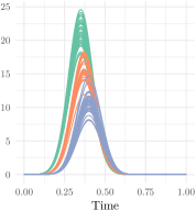
(a) Original Functions

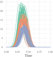
(b) Warped Functions

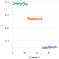
(c) Response Variable

Figure 2: Simulated regression data with phase and amplitude variability.

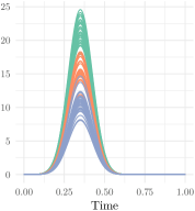
(a) Original Functions

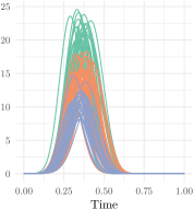
(b) Warped Functions

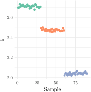
(c) Response Variable

Figure 3: Simulated regression data with amplitude variability.

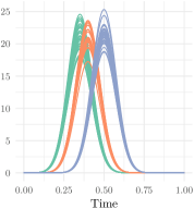
(a) Original Functions

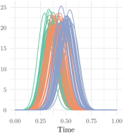
(b) Warped Functions

(c) Response Variable

Figure 4: Simulated regression data with phase variability.

Table 2: Calculated SSE values using four different functional PCR methods for 3 different types of variability.

	Elastic Combined	Elastic Vertical	Elastic Horizontal	Standard
Combined	0.0875 (0.0237)	0.3498 (0.1248)	0.0838 (0.0300)	0.5075 (0.1483)
Vertical	0.2345 (0.0905)	0.2390 (0.0869)	2.0782 (1.9058)	0.3173 (0.0393)
Horizontal	0.1474 (0.0998)	9.1292 (5.3023)	0.2155 (0.1339)	1.8729 (1.1719)

Table 2provides the SSE for each of the three cases with the lowest SSE shown in bold for the applied fPCR method. For the data with the combined variability the combined fPCA in the elastic fPCR model is slightly out performed by the horizontal fPCA. In the cases with the vertical and horizontal variability, the combined elastic fPCA method performed the best with the corresponding vertical or horizontal fPCA method being very close. This is somewhat to be expected as the combined fPCA method is able to capture both types of variability. We compared the results from the elastic method to those using standard fPCR found in the literature on the warped data and is shown in the last column. In all cases the elastic method outperforms the standard fPCR method presented by Reiss and Ogden (2007).

5.2 Elastic Logistic fPCR

To illustrate the developed elastic functional logistic regression method, we evaluated the model on a similar simulated data used in the previous section. The means were chosen according to three models: 1) Combined Amplitude & Phase Variability ($\mu_{j}\in[0.35,0.37]$ and $d_{j}\in[4,3]$), 2. Amplitude Variability ($\mu_{j}\in[0.35,0.35]$ and $d_{j}\in[4,3.7]$), and 3) Phase Variability ($\mu_{j}\in[0.35,0.40]$ and $d_{j}\in[4,4]$). A total of 20 functions were generated for each case and $\sigma=0.075$. The functions were then randomly warped to generate the warped data; $\{f_{i}\}$ and the label was 1 for the first case and -1 for the second case.

Table 3provides the combined probability of classification (PC) for each of the three cases. For the data with the combined variability the combined fPCA in the elastic logistic fPCR model performed the best. In the cases with the vertical and horizontal variability, the corresponding elastic fPCA methods performed well with the combined fPCA method and showed the best performance. We compared the results to the standard logistic fPCR, where the logistic link function is applied to the method of Reiss and Ogden (2007). The results are shown in the last column. In all cases the elastic method outperforms the standard logistic fPCR method.

Table 3: Calculated combined probability of classification values using four different functional PCR methods, for 3 different types of variability for logistic regression.

	Elastic Combined	Elastic Vertical	Elastic Horizontal	Standard
Combined	0.9750 (0.0342)	0.9375 (0.0765)	0.9750 (0.0342)	0.9625 (0.0342)
Vertical	0.9250 (0.0280)	0.8500 (0.0948)	0.6250 (0.0625)	0.8750 (0.0442)
Horizontal	0.9250 (0.0815)	0.6000 (0.1630)	0.8875 (0.1355)	0.8750 (0.0442)

5.3 Elastic Multinomial Logistic fPCR

To illustrate the developed elastic functional regression method we evaluated the model on the simulated data constructed in the elastic functional PCR case. Each of the functions was randomly warped similar to the previous cases. The response variable $y_{i}$ in this case was categorical with values $j\in\{1,2,3\}$ depending on the corresponding model.

Table 4provides the combined probability of classification (PC) for each of the three cases. For the data with the combined variability the horizontal and combined fPCA in the elastic multinomial logistic fPCR model performed the best. In the cases with the vertical and horizontal variability, the corresponding elastic fPCA methods performed the well with the combined fPCA method having the best performance. We compared the results to using standard multinomial logistic fPCR found in the literature on the warped data and is presented in the last column. In all cases the elastic method outperforms the standard multinomial logistic fPCR method.

Table 4: Calculated combined probability of classification values using four different functional PCR methods, for 3 different types of variability for multinomial logistic regression.

	Elastic Combined	Elastic Vertical	Elastic Horizontal	Standard
Combined	0.9420 (0.0633)	0.9246 (0.0355)	0.9670 (0.0348)	0.8663 (0.1597)
Vertical	0.8589 (0.0801)	0.8916 (0.0229)	0.3822 (0.0710)	0.8749 (0.0780)
Horizontal	0.9176 (0.0480)	0.3822 (0.1036)	0.9666 (0.0187)	0.9510 (0.0436)

6 Applications to Real Data

Here, we present the results on multiple real data sets for the three elastic regression models. For the elastic fPCR we use the Sonar data set presented in (Tucker et al. (2014)) where we predict the volumes of two targets. We demonstrate the elastic logistic fPCR model on four sets. The data consists of physiological data, specifically, gait and electrocardiogram (ECG) measurements from various patients. Phase-variability is naturally found in the data, as during collection the signals always start and stop at the different time for each measurement. For example, when measuring a heart beat one cannot assure that the measurement starts on the same part of the heartbeat for each patient measured. For the elastic multinomial logistic fPCR model we demonstrate on two sets that consist of physiologic data similar to those used to test the logistic regression method.

6.1 Sonar Data

The data set used in these experiments was collected at the Naval Surface Warfare Center Panama City Division (NSWC PCD) test pond. For a description of the pond and a similar experimental setup the reader is referred to Kargl et al. (2010). The raw SONAR data was collected using a 1 - 30$kHz$ LFM chirp and data was collected for a solid aluminum cylinder and an aluminum pipe. The aluminum cylinder is 2$ft$ long with a 1$ft$ diameter; while the pipe is 2$ft$ long with an inner diameter of 1$ft$ and 3/8 inch wall thickness. During the experiment the targets were placed with added uncertainty of their orientation. The acoustic signals were generated from the raw SONAR data to construct target strength as a function of frequency and aspect angle.

Figure 5(a) presents the original functions for the acoustic color measurements at $0^{\circ}$ aspect angle. There appears to be significant amplitude and phase variability between functional measurements due to experimental collection uncertainty. Not accounting for the phase variability can greatly affect summary statistics and follow-on statistical models. Figure 5(b) and (c) show the aligned functions (amplitude) and warping functions (phase), respectively. Overall there is significant difference between the original functions and the aligned functions. With the large amount of phase variability, the frequency structure of the data was lost. As a result, cross-sectional methods without alignment will not capture this important difference in the functions.

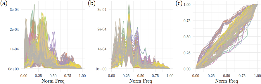
Figure 5: Alignment of the sonar dataset. (a) Original functions. (b) Aligned functions (amplitude). (c) Warping functions (phase).

Table 5: Calculated SSE values using four different functional PCR methods for the sonar data set.

	Elastic Combined	Elastic Vertical	Elastic Horizontal	Standard
SSE	0.1210 (0.0472)	0.1497 (0.1399)	0.1597 (0.0485)	0.1908 (0.1184)

Table 5presents the sum of squared errors (SSE) calculated using 5-fold cross-validation. For this data set, we use ten principal components resulting in a ten-dimensional model for all four methods. In the table we present the mean of the SSE across the folds, along with the standard deviation. We compare the three elastic versions and standard functional principal component regression; the lowest SSE is shown in bold. The lowest SSE is the combined elastic fPCR method and all three elastic methods have lower SSE than the standard method in predicting the volume from the sonar data. With the high degree of phase and amplitude variability in the data, the elastic method is more able to accurately predict and capture the variability.

6.2 Gait Data

The Gait data is a collection of gait measurements for patients having Parkinson’s disease, and those not having Parkinson’s disease. It is from the gaitpdb data set on Physionet (Goldberger et al. (2000)). This database contains measures of gait from 93 patients with idiopathic Parkinson’s disease and 73 healthy patients. The gait was measured using vertical ground reaction force records of subjects as they walked at their usual, self-selected pace for approximately 2 minutes on level ground.

Figure 6(a) presents the original functions for gait data and are colored for the two different classes. There appears to be significant amplitude and phase variability between functional measurements due to experimental collection uncertainty and where one subject will start and stop their gate. Figure 6(b) and (c) show the aligned functions (amplitude) and warping functions (phase), respectively. Overall there is significant difference between the original functions and the aligned functions. With the large amount of phase variability, the temporal structure of the gaits will be lost in the analysis. As a result, cross-sectional methods without alignment will not capture this important difference in the functions.

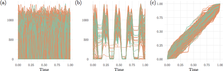
Figure 6: Alignment of the gait data dataset. (a) Original functions. (b) Aligned functions (amplitude). (c) Warping functions (phase).

The first row in Table 6presents the calculated mean probability of classification (PC) using 5-fold cross-validation. For this data set, we use five principal components resulting in a five-dimensional model for all four methods. In the table we present the mean of the PC across the folds, along with the standard deviation. We compare the three elastic versions and standard logistic fPCR and the largest PC is shown in bold. The largest PC is the vertical elastic logistic fPCR method. All three elastic methods have higher PC than the standard method for predicting if the subject has Parkinson’s based on gait measurement. This suggests that a large portion of the information is contained in the amplitude variability.

6.3 ECG200 Data

The ECG200 data is a collection of ECG measurements of heartbeats demonstrating an arrhythmia, and those which do not. The data set is from the MIT-BIH Arrhythmia Database available from Physionet. The database contains ECG recordings where each electrocardiogram was recorded from a single patient for a duration of approximately thirty minutes. From the recordings heartbeats were extracted with the most prevalent abnormality—supra-ventricular premature beat. Additionally, heartbeats were extracted from the recordings that were representative of normal heartbeats. The task is then to distinguish between the abnormalities using the heartbeat. Naturally, the heartbeats are not aligned and no alignment was made to the data.

Figure 7(a) presents the original electrocardiogram measurements. There appears to be significant phase variability between functional measurements due to timing uncertainty across collections. Figure 7(b) and (c) show the aligned functions (amplitude) and warping functions (phase), respectively.

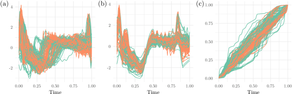
Figure 7: Alignment of the ECG200 data dataset. (a) Original functions. (b) Aligned functions (amplitude). (c) Warping functions (phase).

The second row in Table 6presents the calculated mean probability of classification (PC) using 5-fold cross-validation. Again for this data set, we use five principal components resulting in a five-dimensional model for all four methods, and present the mean of the PC across the folds; along with the standard deviation. The largest PC is the vertical elastic logistic fPCR method. All three elastic methods have higher PC than the standard method, however, for this data it performs quite well.

6.4 TwoLead ECG Data Set

The TwoLead ECG data set, is a collection of ECG measurements from the MIT-BIH Long-Term ECG Database available as well from Physionet. These contains long term ECG measurements with beat annotations. Heartbeats were extracted that were annotated normal and abnormal for the two classes.

Figure 8(a) presents the original electrocardiogram measurements. Again, there appears to be significant phase variability between functional measurements due to timing uncertainty across collections. Figure 8(b) and (c) show the aligned functions (amplitude) and warping functions (phase), respectively. Overall there is a noticeable alignment and better definition of the wave structure.

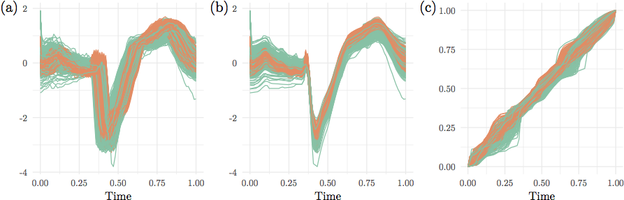
Figure 8: Alignment of the TwoLead ECG data dataset. (a) Original functions. (b) Aligned functions (amplitude). (c) Warping functions (phase).

The third row in Table 6presents the calculated mean probability of classification (PC) using 5-fold cross-validation. Again for this data set, we use five principal components resulting in a five-dimensional model for all four methods and present the mean of the PC across the folds, along with the standard deviation. The largest PC is the vertical elastic logistic fPCR method and all three elastic methods have higher PC than the standard method.

6.5 ECGFiveDays Data Set

The ECGFiveDays data set, is a collection of ECG measurements from a 67 year old male. There are two classes which are simply the data of the ECG measurements which are 5 days apart. The task is then to distinguish between the two days, as the wandering baseline was not removed and the heartbeats are not aligned. The data set is the ECGFiveDays from the UCR Time Series Classification Database (Keogh et al. (2001)). Moreover, the previous two data sets can also be obtained from the UCR database under the names ECG200 and TwoLeadECG, respectively.

Figure 9(a) presents the original electrocardiogram measurements from the ECGFiveDays set. Again, there appears to be some phase variability between functional measurements due to timing uncertainty across collections. Figure 9(b) and (c) show the aligned functions (amplitude) and warping functions (phase), respectively. Overall there is a noticeable alignment and separation of the two classes in both the aligned functions and the warping functions.

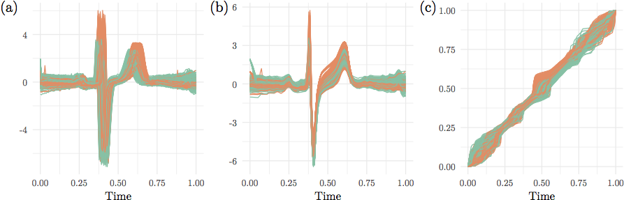
Figure 9: Alignment of the ECGFiveDays data dataset. (a) Original functions. (b) Aligned functions (amplitude). (c) Warping functions (phase).

Table 6: Calculated probability of correct classification using four different functional logistic fPCR methods for four different data sets.

	Elastic Combined	Elastic Vertical	Elastic Horizontal	Standard
Gait	0.6467 (0.0321)	0.6900 (0.0465)	0.6333 (0.0425)	0.4300 (0.0923)
ECG200	0.7750 (0.0791)	0.8350 (0.0675)	0.7450 (0.0716)	0.8200 (0.0694)
TwoLead ECG	0.9113 (0.0125)	0.9845 (0.0163)	0.9156 (0.0146)	0.8012 (0.0133)
ECGFiveDays	0.9570 (0.0228)	0.8902 (0.0462)	0.8473 (0.0429)	0.9061 (0.0297)

The last row in Table 6presents the calculated mean probability of classification (PC) using 5-fold cross-validation. Again for this data set, we use five principal components resulting in a five-dimensional model for all four methods. We present the mean of the PC across the folds, along with the standard deviation. The largest PC is the combined elastic fPCR method and all three elastic methods have higher PC than the standard method. This suggests that there is a combination of both phase and amplitude that contribute to correct classification.

6.6 Gaitndd Data set

The Gaitndd data set is a collection of gait measurements for patients having Parkinson’s disease, Amyotrophic lateral sclerosis, Huntington’s disease, and healthy controls; and is from the gaitndd data set on Physionet (Goldberger et al. (2000)). This database contains measures of gait from 15, 20, 13, and 16 patients for the respective diseases. The gait was measured using vertical ground reaction force records of subjects as they walked at their usual pace.

Figure 10(a) presents the original gait measurements and are colored for the different classes. There is a large phase and amplitude variability between functional measurements. Figure 10(b) and (c) show the aligned functions (amplitude) and warping functions (phase), respectively. Overall there is a large improvement in the structure after alignment, and some class definition can be noticed in the functions.

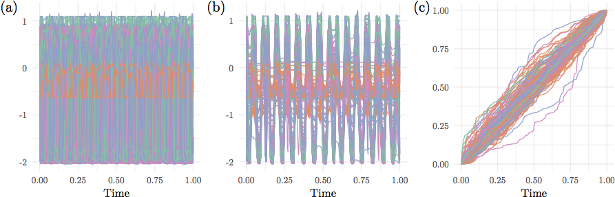
Figure 10: Alignment of the Gaitndd data dataset. (a) Original functions. (b) Aligned functions (amplitude). (c) Warping functions (phase).

The first row in Table 7presents the calculated mean probability of classification (PC) using 5-fold cross-validation. For this data set, we use ten principal components resulting in a ten-dimensional model for all four methods. We then present the mean of the PC across the folds, along with the standard deviation. The largest PC is the vertical elastic fPCR method and all three elastic methods have higher PC than the standard method. This suggests there is a large amplitude component in how each disease affects the gait.

6.7 CinC ECG Data Set

The last data set is a collection of ECG measurements from multiple torso-surface sites. There are measurements from 4 different people who are the 4 different classes. The data set is from the 2007 Physionet CinC challenge and is also found as the CinC data set from the UCR Time Series Classification Database (Keogh et al. (2001)).

Figure 11(a) presents the original ECG measurements and are colored for the different classes. There is a large phase and amplitude variability between functional measurements. Figure 11(b) and (c) show the aligned functions (amplitude) and warping functions (phase), respectively. Overall there is a large improvement in the structure after alignment and noticeable class separation in the warping functions. This suggests that the phase will have a large contribution to the classification.

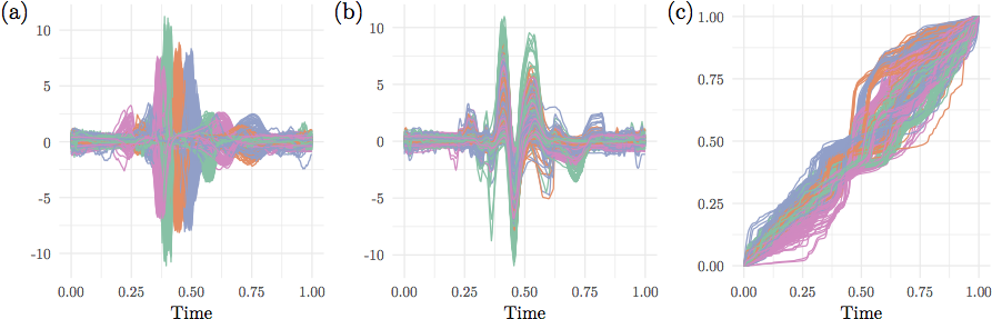
Figure 11: Alignment of the CinC ECG data dataset. (a) Original functions. (b) Aligned functions (amplitude). (c) Warping functions (phase).

Table 7: Calculated probability of correct classification using four different functional multinomial logistic fPCR methods for two different data sets.

	Elastic Combined	Elastic Vertical	Elastic Horizontal	Standard
Gaitndd	0.3949 (0.0648)	0.4888 (0.0326)	0.3645 (0.0398)	0.3123 (0.0413)
CinC ECG	0.6785 (0.0403)	0.6342 (0.0311)	0.6954 (0.0452)	0.3297 (0.0374)

The last row in Table 7presents the calculated mean probability of classification (PC) using 5-fold cross-validation. For this data set, we use ten principal components resulting in a ten-dimensional model for all four methods and present the mean of the PC across the folds, along with the standard deviation. The largest PC is the horizontal elastic fPCR method, and all three elastic methods have higher PC than the standard method. This suggests there is a large phase component in the classification performance. When accounting for this performance of correct classification is dramatically larger than just performing standard multinomial functional principal component regression.

7 Conclusion and Future Work

The statistical modeling and classification of functional data with phase variability is a challenging task. We have proposed a new functional principal component regression approach, that addresses the problem of registering and modeling functions in one elastic-framework. We demonstrated three PCA methods: 1) combined, 2) vertical, and 3) horizontal that can be used depending on the type of data encountered. This enabled the implementation of a regression model that is geometrically-motivated. We demonstrated the applicability of these to models on a three different simulated examples, that contain different types of variability. We also tested seven real data examples with significant amplitude and phase variabilities. In all cases, we illustrated improvements in prediction power of the proposed models.

We have identified several directions for future work. First, we will explore the influence of the weight $C$ in the combined amplitude and phase fPCA model on the resulting regression model performance. Second, in many applications, the functional data of interest may be more complex than the simple univariate functions considered in this work; some examples include shapes of curves, surfaces, and images. These more complicated data objects often exhibit different sources of variability, which must be taken into account when computing regression models.

References

- Bhattacharya (1943) Bhattacharya, A. (1943). On a measure of divergence between two statistical populations defined by their probability distributions. Bull. Calcutta Math. Soc. 35, 99–109.
- Byrd et al. (1995) Byrd, R. H., P. Lu, J. Nocedal, and C. Zhu (1995). A limited memory algorithm for bound constrained optimization. SIAM J. Sci. Comput. 16(5), 1190–1208.
- Cai and Hall (2006) Cai, T. and P. Hall (2006). Prediction in functional linear regression. Annals of Statistics 34(5), 2159–2179.
- Cardot et al. (1999) Cardot, H., F. Ferraty, and P. Sarda (1999). Functional linear model. Statistics & Probability Letters 45, 11–22.
- Cardot et al. (2003) Cardot, H., F. Ferraty, and P. Sarda (2003). Spline estimator for the functional linear model. Statistica Sinica 13, 571–591.
- Carroll et al. (2006) Carroll, R. J., D. Ruppert, L. A. Stefanski, and C. M. Crainiceanu (2006). Measurement Error in Nonlinear Models: A Modern Perspective (2 ed.). Chapman and Hall/CRC.
- Cuevas et al. (2002) Cuevas, A., M. Febrero, and R. Fraiman (2002). Linear functional regression; the case of fixed design and functional response. The Canadian Journal of Statistics 30, 285–300.
- Gertheiss et al. (2013) Gertheiss, J., A. Maity, and A.-M. Staicu (2013). Variable selection in generalized functional linear models. Stat 2(1), 86–101.
- Gervini (2015) Gervini, D. (2015). Curve registration. Biometrika 102(1), 1–14.
- Goldberger et al. (2000) Goldberger, A. L., L. A. N. Amaral, L. Glass, J. M. Hausdorff, P. C. Ivanov, R. G. Mark, J. E. Mietus, G. B. Moody, C. Peng, and H. E. Stanley (2000, June). Physiobank, physiotoolkit, and physionet: Components of a new research resource for complex physiologic signals. Circulation 101(23), e215–e220.
- Hall and Horowitz (2007) Hall, P. and J. L. Horowitz (2007). Methodology and convergence rates for functional linear regression. Annals of Statistics 35(1), 70–91.
- James (2002) James, G. M. (2002). Generalized linear models with functional predictors. Journal of the Royal Statistical Society: Series B 64, 411–432.
- James et al. (2009) James, G. M., J. Wang, and J. Zhu (2009). Functional linear regression that’s interpretable. Anals of Statistics 37(5A), 2083–2108.
- Jung et al. (2012) Jung, S., I. L. Dryden, and J. S. Marron (2012). Analysis of principal nested spheres. Biometrika 99(3), 551–568.
- Kargl et al. (2010) Kargl, S., K. Williams, T. Marston, J. Kennedy, and J. Lopes (2010). Acoustic response of unexploded ordnance (UXO) and cylindrical targets) and cylindrical targets. Proc. of MTS/IEEE Oceans 2010 Conference, 1 –5.
- Keogh et al. (2001) Keogh, E., Q. Zhu, B. Hu, Y. Hao, X. Xi, L. Wei, and C. A. Ratanamahatana (2001). The UCR time series classification/clustering homepage.
- Kurtek (2017) Kurtek, S. (2017). A geometric approach to pairwise Bayesian alignment of functional data using importance sampling. Electronic Journal of Statistics 11(1), 502–531.
- Kurtek and Bharath (2015) Kurtek, S. and K. Bharath (2015). Bayesian sensitivity analysis with Fisher–Rao metric. Biometrika 102(3), 601–616.
- Kurtek et al. (2011) Kurtek, S., A. Srivastava, and W. Wu (2011). Signal estimation under random time-warpings and nonlinear signal alignment. In Proceedings of Neural Information Processing Systems (NIPS).
- Lahiri et al. (2015) Lahiri, S., D. Robinson, and E. Klassen (2015). Precise matching of PL curves in in the Square Root Velocity framework. Geometry, Imaging and Computing 2, 133–186.
- Lee and Jung (2017) Lee, S. and S. Jung (2017). Combined analysis of amplitude and phase variations in functional data. arXiv:1603.01775 [stat.ME], 1–21.
- Lu et al. (2017) Lu, Y., R. Herbei, and S. Kurtek (2017). Bayesian registration of functions with a Gaussian process prior. Journal of Computational and Graphical Statistics 26(4), 894–904.
- Marron et al. (2015) Marron, J. S., J. Ramsay, L. Sangalli, and A. Srivastava (2015). Functional data analysis of amplitude and phase variation. Statistical Science 30(4), 468–484.
- Mordecai (2003) Mordecai, A. (2003). Nonlinear Programming: Analysis and Methods. Dover Publishing.
- Müller and Stadtmüller (2005) Müller, H. G. and U. Stadtmüller (2005). Generalized functional linear models. Annals of Statistics 33(2), 774–805.
- Ramsay and Dalzell (1991) Ramsay, J. O. and C. J. Dalzell (1991). Some tools for functional data analysis. Journal of the Royal Statistical Society, Ser. B 53(3), 539–572.
- Ramsay and Silverman (2005) Ramsay, J. O. and B. W. Silverman (2005). Functional Data Analysis. Springer.
- Reiss and Ogden (2007) Reiss, P. and R. Ogden (2007). Functional principal component regression and functional partial least squares. Journal of American Statistical Association 102(479), 984–996.
- Robinson (2012) Robinson, D. (2012). Functional analysis and partial matching in the square root velocity framework. Ph. D. thesis, Florida State University.
- Srivastava and Jermyn (2009) Srivastava, A. and I. H. Jermyn (2009). Looking for shapes in two-dimensional, cluttered point clouds. IEEE Trans. Pattern Analysis and Machine Intelligence 31(9), 1616–1629.
- Srivastava et al. (2005) Srivastava, A., S. H. Joshi, W. Mio, and X. Liu (2005). Statistical shape analysis: Clustering, learning and testing. IEEE Trans. Pattern Analysis and Machine Intelligence 27(4), 590–602.
- Srivastava et al. (2011) Srivastava, A., E. Klassen, S. Joshi, and I. Jermyn (2011). Shape analysis of elastic curves in euclidean spaces. IEEE Trans. Pattern Analysis and Machine Intelligence 33(7), 1415–1428.
- Srivastava et al. (2011) Srivastava, A., W. Wu, S. Kurtek, E. Klassen, and J. S. Marron (2011). Registration of functional data using fisher-rao metric. arXiv:1103.3817v2 [math.ST].
- Tucker et al. (2013) Tucker, J. D., W. Wu, and A. Srivastava (2013). Generative models for functional data using phase and amplitude separation. Computational Statistics and Data Analysis 61, 50–66.
- Tucker et al. (2014) Tucker, J. D., W. Wu, and A. Srivastava (2014). Analysis of signals under compositional noise with applications to sonar data. IEEE Journal of Oceanic Engineering 39(2), 318–330.
- Veeraraghavan et al. (2009) Veeraraghavan, A., A. Srivastava, A. K. Roy-Chowdhury, and R. Chellappa (2009). Rate-invariant recognition of humans and their activities. IEEE Transactions on Image Processing 8(6), 1326–1339.