Analysis of the energy dissipation laws in multi-component phase field models

Abstract

In this paper, two approaches for modeling three-component fluid flows using diffusive interface method are discussed. Thermodynamic consistency of the proposed models is preserved when using an energetic variational framework to derive the coupled systems of partial differential equations that comprise the resulting models. The issue of algebraic and dynamic consistency is investigated. In addition, the two approaches that are presented are compared analytically and numerically.

1 Introduction

Interface problems arising in mixtures of different fluids, solids and gases have attracted attention for more than two centuries. Many surface properties, such as capillarity, are associated with the surface tension through special boundary conditions [25, 24].

Figure 1: Schematic representation of a binary mixture.

The classical approach to this problem usually considers the interface to be a free surface that evolves in time with the fluid velocity [20]. In this approach the so-called sharp interface problem for the immiscible mixture of two fluids is written as Navier-Stokes equation in each component with stress jump conditions on the moving interface (see fig. 1). This approach results in the system that satisfies the following energy law:

$$\frac{d}{dt}\left[\sum_{i=1,2}\int_{\Omega_{i}}\frac{1}{2}\rho\left|\mathbf{u}^{i}\right|d\mathbf{x}+\sigma\ \text{area}\Gamma_{t}\right]=-\sum_{i=1,2}\int_{\Omega_{i}}2\eta_{i}\left|\frac{\nabla\mathbf{u}^{i}+\left(\nabla\mathbf{u}^{i}\right)^{T}}{2}\right|^{2}d\mathbf{x}.$$ (1)

Here $\Omega_{i}$ are the sub-domains corresponding to each component of the mixture, $\mathbf{u}^{i}$ and $\eta_{i}$ are local velocities and viscosities of each component, $\sigma$ is the surface tension constant, and $\Gamma_{t}$ is the moving interface between the components.

Energetic Variational Approach

The models presented in this paper are derived from the underlying energetic variational structures. For an isothermal closed system, the combination of the First and Second Laws of Thermodynamics yields the following energy dissipation law [19]:

$$\frac{dE^{\rm total}}{dt}=-\Delta,$$ (2)

where $E^{\rm total}$ is the sum of kinetic energy and the total Helmholtz free energy, and $\Delta$ is the entropy production (here the rate of energy dissipation). The choices of the total energy functional and the dissipation functional, together with the kinematic (transport) relations of the variables employed in the system, determine all the physical and mechanical considerations and assumptions for the problem.

The Energetic Variational Approach (EnVarA) is motivated by the seminal works of Rayleigh [38] and Onsager [36, 35]. The framework, including Least Action Principle (LAP) and Maximum Dissipation Principle (MDP), provides a unique, well defined, way to derive the coupled dynamical systems from the total energy functionals and dissipation functions in the dissipation law (2) [22]. Instead of using the empirical constitutive equations, the force balance equations are derived. Specifically, the Least Action Principle determines the Hamiltonian part of the system [3, 1] and the Maximum Dissipation Principle accounts for the dissipative part [36, 4]. Formally, LAP represents the fact that the force multiplied by the distance is equal to the work, i.e., $\delta E={\rm force}\times\delta x,$ where $x$ is the location and $\delta$ the variation/derivative. This procedure gives the conservative forces. The MDP, by Onsager and Rayleigh, produces the dissipative forces of the system, $\delta\frac{1}{2}\Delta={\rm force}\times\delta{\dot{x}}.$ The factor $\frac{1}{2}$ is consistent with the choice of quadratic form for the “rates” that describe the linear response theory for long-time near equilibrium dynamics [29].

Both total energy and energy dissipation may contain terms related to microstructure and those describing macroscopic flow. Competition between different parts of energy, as well as energy dissipation defines the dynamics of the system. For more details see [19].

Diffuse Interface Method

To regularize the transition between two phases in the sharp interface model here the statistical point of view (or phase field approach) is employed, which treats the interface as a continuous, but steep, change of properties (density, viscosity etc) of the two fluids. Within a “thin” transition region, the fluid is mixed and has to store certain amount of “mixing energy”. Such an approach coincides with the usual phase field models in the theory of phase transition [10, 9]. These models will allow the topological change of the interface [33], and have many advantages when simulating front motions [12]. Recently many researchers have employed the phase field approach for various fluid models [23, 21, 2, 32, 5, 37, 31].

Figure 2: Configuration of a phase field function $\varphi$ describing two phase flow.

The phase field function $\varphi$ takes values $\varphi=1$ in $\Omega_{1}$, $\varphi=-1$ in $\Omega_{2}$, and $\varphi\in\left(-1,\,1\right)$ on the diffusive interface. We use phase field to approximate the interface energy with mixing energy

$$\frac{\lambda}{\sigma}\mathcal{W}\left(\varphi\right)=\frac{\lambda}{\sigma}\int\frac{\varepsilon}{2}\left|\nabla\varphi\right|^{2}+\frac{1}{\varepsilon}G\left(\varphi\right)d\mathbf{x}\approx\text{area}\Gamma_{t},$$ (3)

where $G$ is a so-called double-well potential (e.g. $G\left(\varphi\right)=\frac{1}{4}\left(\varphi^{2}-1\right)^{2}$), $\varepsilon$ is a parameter responsible for the “width” of the interface, and $\lambda/\sigma$ depends on $G\left(\varphi\right)$ (for example, $\lambda=\frac{3}{2\sqrt{2}}\sigma$ if $G\left(\varphi\right)=\frac{1}{4}\left(\varphi^{2}-1\right)^{2}$, where $\sigma$ is the surface tension constant, see [40]).

Then the energy law for two-component fluid flow

$$\frac{d}{dt}\left(\int\frac{1}{2}\rho\left|\mathbf{u}\right|^{2}d\mathbf{x}+\lambda\mathcal{W}\left(\varphi\right)\right)=-\int\frac{1}{2}\eta\left|\nabla\mathbf{u}+\nabla\mathbf{u}^{T}\right|^{2}+\frac{\varphi^{2}}{M\left(\varphi\right)}\left|\mathbf{V}-\mathbf{u}\right|^{2}d\mathbf{x},$$ (4)

combined with kinematic constraint $\varphi_{t}+\nabla\cdot\left(\varphi\mathbf{V}\right)=0$ and incompressibility condition $\nabla\cdot\mathbf{u}=0$ after applying EnVarA gives way to the following Cahn-Hilliard/Navier-Stokes system:

$$\begin{cases}\varphi_{t}+\nabla\cdot\left(\varphi\mathbf{u}\right)=\nabla\cdot\left(M\left(\varphi\right)\nabla\zeta\right),\quad\zeta=-\lambda\varepsilon\Delta\varphi+\lambda\frac{1}{\varepsilon}\left(\varphi^{2}-1\right)\varphi,\\ \rho\left(\mathbf{u}_{t}+\left(\mathbf{u}\cdot\nabla\right)\mathbf{u}\right)+\nabla p=\nabla\cdot\left[\eta\left(\nabla\mathbf{u}+\left(\nabla\mathbf{u}\right)^{T}\right)-\lambda\varepsilon\nabla\varphi\otimes\nabla\varphi\right],\\ \nabla\cdot\mathbf{u}=0.\end{cases}$$ (5)

For more details see [19].

Multi-component mixtures

The phase field model for ternary mixtures is much less studied in comparison to its binary analog. It was first introduced by Morral and Cahn [34] and later developed by several works [16, 17, 18, 28, 6, 8, 41].

In [6] for a phase field model based on concentrations authors introduce consistency requirements that should be imposed on the ternary model (we shall call this approach “non-degenerate”). They analyze the energy law and resulting system and derive constraints to satisfy the requirements. This and positivity of the proposed energy limit the range of physical parameters. In [8] authors introduce a phase field model that does not require imposing limits on physical parameters (we shall call this approach “degenerate” for the degeneracy in one of the coefficients in the energy law).

In section 2 we introduce the Cahn-Hilliard models based on the aforementioned approaches. In section 3.1 we analyze the consistency requirements for the “degenerate” model. In section 3.2 we compare the energies and dynamics of the systems between the two approaches.

2 Models of Multi-component Flows

The phase field modeling of three-component dynamics can be divided into two distinct approaches, which we call non-degenerate [27, 26, 6, 41, 14] and degenerate (for the degeneracy in the dynamics of one of the components) [8, 7]. With the energetic variational approach the main requirement for any such model is that in the absence of one of the phases, the postulated mixing energy reduces to that of the two-phase flow (energetic consistency). Additionally, in [6] authors suggested, that such requirement should be imposed not just on the energy, but on the dynamics of the system as well (algebraic consistency) and that this property should hold under small perturbations (dynamic consistency). Similar to two-component flow, we postulate the following generic energy law:

$$\frac{d}{dt}\left(\int\frac{1}{2}\rho\left|\mathbf{u}\right|^{2}d\mathbf{x}+\mathcal{W}\right)=-2\mathcal{D},$$ (6)

Different models may be obtained by introducing different mixing energies $\mathcal{W}$ and dissipation functionals $\mathcal{D}$. We briefly describe two approaches, discuss the differences in their postulated mixing energies and resulting dynamics and investigate requirements on the energy for the degenerate system to satisfy the dynamic consistency requirement without any limitations on the mobility coefficients.

Non-degenerate system

Let us introduce a phase field vector $\mathbf{c}=\left<c_{1},\,c_{2},\,c_{3}\right>$, where each component of the vector may be thought of as relative concentration (or relative

Figure 3: Configuration of a phase field vector $\mathbf{c}=\left<c_{1},\,c_{2},\,c_{3}\right>=\left<c,\,d,\,1-c-d\right>$ describing three phase flow.

density) of the corresponding phase. Then we can write the mixing energy as follows:

$$\mathcal{W}\left(\mathbf{c}\right)=\int\frac{3}{8}\varepsilon\sum_{i=1}^{3}\chi_{i}\left|\nabla c_{i}\right|^{2}+\frac{12}{\varepsilon}F\left(\mathbf{c}\right)d\mathbf{x},$$ (7)

where $F\left(\mathbf{c}\right)$ is a triple-well potential, that may be taken of different forms, and constants $\chi_{i}$ are related to penetration constants in capillarity theory and may be expressed through surface tension constants of the three interfaces using the energetic consistency requirement.

Here we introduce the following dissipation functional

$$\mathcal{D}=\int\frac{1}{4}\eta\left|\nabla\mathbf{u}+\nabla\mathbf{u}^{T}\right|^{2}+\sum_{i=1}^{3}\frac{c_{i}^{2}}{2M_{i}}\left|\mathbf{V}_{i}-\mathbf{u}\right|^{2}d\mathbf{x},$$ (8)

together with kinematic relations $c_{i\,t}+\nabla\cdot\left(c_{i}\mathbf{V}_{i}\right)=0,\ i=1,2,3$, and incompressibility constraint $\nabla\cdot\mathbf{u}=0$. In addition, the concentrations are related by a linear constraint $c_{1}+c_{2}+c_{3}=1$. In order to satisfy the algebraic consistency, authors of [6] perform the variation with Lagrange multiplier $\beta$ and algebraic restrictions on mobility coefficients $M_{i}$ to derive the following ternary Cahn-Hilliard/Navier-Stokes system:

$$\begin{cases}c_{t}+\left(\mathbf{u}\cdot\nabla\right)c=M_{1}\Delta\zeta_{c},\quad\zeta_{c}=-\frac{3}{4}\varepsilon\nabla\cdot\left(\chi_{1}\nabla c\right)+\frac{12}{\varepsilon}\partial_{1}F\left(\mathbf{c}\right)+\beta,\\ d_{t}+\left(\mathbf{u}\cdot\nabla\right)d=M_{2}\Delta\zeta_{d},\quad\zeta_{d}=-\frac{3}{4}\varepsilon\nabla\cdot\left(\chi_{2}\nabla d\right)+\frac{12}{\varepsilon}\partial_{2}F\left(\mathbf{c}\right)+\beta,\\ \beta=-\frac{12}{\varepsilon}\chi_{0}\left(\frac{1}{\chi_{1}}\partial_{1}F\left(\mathbf{c}\right)+\frac{1}{\chi_{2}}\partial_{2}F\left(\mathbf{c}\right)+\frac{1}{\chi_{3}}\partial_{3}F\left(\mathbf{c}\right)\right),\\ \rho\left(\mathbf{u}_{t}+\left(\mathbf{u}\cdot\nabla\right)\mathbf{u}\right)+\nabla p=\nabla\cdot\left[\eta\left(\nabla\mathbf{u}+\left(\nabla\mathbf{u}\right)^{T}\right)-\frac{3}{4}\varepsilon\sum_{i=1}^{3}\chi_{i}\nabla c_{i}\otimes\nabla c_{i}\right],\\ \nabla\cdot\mathbf{u}=0,\\ \mathbf{c}=\left\langle c_{1},\,c_{2},\,c_{3}\right\rangle=\left\langle c,\,d,\,1-c-d\right\rangle,\\ \chi_{0}=\left(\chi_{1}^{-1}+\chi_{2}^{-1}+\chi_{3}^{-1}\right)^{-1},\quad M_{1}\chi_{1}=M_{2}\chi_{2}=M_{3}\chi_{3}=M_{0}.\end{cases}$$ (9)

Dynamic consistency requires additional restrictions on the choice of nonlinear potential $F\left(\mathbf{c}\right)$.

Figure 4: Configuration of a phase field functions $\varphi$ and $\psi$ describing ternary flow.

Degenerate system

In the degenerate approach, instead of three linearly dependent functions, we introduce two completely independent phase field functions $\varphi$ and $\psi$, which act as labels. Two of the components are distinguished from each other using values of $\varphi$, while third component is distinguished from both of the first two using values of $\psi$ (see Fig. 4). Then the mixing energy will have a term acting on the interface of the first two components in the region with $\psi=1$, and another term on the interface separating third component from both of the first two:

$$\mathcal{W}\left(\varphi,\psi\right)=\int \widetilde{\gamma}_{1}\left(\psi\right)\left(\frac{\psi+1}{2}\right)^{2}\left(\frac{\varepsilon}{2}\left|\nabla\varphi\right|^{2}+\frac{1}{4\varepsilon}\left(1-\varphi^{2}\right)^{2}\right)$$

$$+\gamma_{2}\left(\varphi\right)\left(\frac{\varepsilon}{2}\left|\nabla\psi\right|^{2}+\frac{1}{4\varepsilon}\left(1-\psi^{2}\right)^{2}\right),$$ (10)

where $\gamma_{1}\left(\psi\right)=\widetilde{\gamma}_{1}\left(\psi\right)\left(\frac{\psi+1}{2}\right)^{2}$ and $\gamma_{2}\left(\varphi\right)$ are coefficients related to the surface tensions on the corresponding interfaces. Writing the dissipation functional as

$$\mathcal{D}=\int\frac{1}{4}\eta\left|\nabla\mathbf{u}+\nabla\mathbf{u}^{T}\right|^{2}+\frac{\varphi^{2}}{2M_{1}}\left|\mathbf{V}_{\varphi}-\mathbf{u}\right|^{2}+\frac{\psi^{2}}{2M_{2}}\left|\mathbf{V}_{\psi}-\mathbf{u}\right|^{2}d\mathbf{x},$$ (11)

and applying energetic variational approach one can derive degenerate ternary Cahn-Hilliard/Navier-Stokes system:

$$\begin{cases}\varphi_{t}+\left(\mathbf{u}\cdot\nabla\right)\varphi=\nabla\cdot\left(M_{1}\nabla\zeta_{\varphi}\right),\quad\psi_{t}+\left(\mathbf{u}\cdot\nabla\right)\psi=\nabla\cdot\left(M_{2}\nabla\zeta_{\psi}\right),\\ \zeta_{\varphi}=-\varepsilon\nabla\cdot\left[\gamma_{1}\left(\psi\right)\nabla\varphi\right]+\frac{1}{\varepsilon}\gamma_{1}\left(\psi\right)\left(\varphi^{2}-1\right)\varphi\\ \hskip 27.0pt+\frac{\partial\gamma_{2}\left(\varphi\right)}{\partial\varphi}\left(\frac{\varepsilon}{2}\left|\nabla\psi\right|^{2}+\frac{1}{4\varepsilon}\left(\psi^{2}-1\right)^{2}\right),\\ \zeta_{\psi}=-\varepsilon\nabla\cdot\left(\gamma_{2}\left(\varphi\right)\nabla\psi\right)+\frac{\gamma_{2}\left(\varphi\right)}{\varepsilon}\left(\psi^{2}-1\right)\psi+\\ \hskip 27.0pt+\frac{\partial\gamma_{1}\left(\psi\right)}{\partial\psi}\left(\frac{\varepsilon}{2}\left|\nabla\varphi\right|^{2}+\frac{1}{4\varepsilon}\left(\varphi^{2}-1\right)^{2}\right),\\ \rho\left(\mathbf{u}_{t}+\left(\mathbf{u}\cdot\nabla\right)\mathbf{u}\right)+\nabla p=\nabla\cdot\left[\eta\left(\nabla\mathbf{u}+\left(\nabla\mathbf{u}\right)^{T}\right)\right.\\ \hskip 60.0pt\left.-\varepsilon\gamma_{1}\left(\psi\right)\left(\nabla\varphi\otimes\nabla\varphi\right)-\varepsilon\gamma_{2}\left(\varphi\right)\left(\nabla\psi\otimes\nabla\psi\right)\right],\\ \nabla\cdot\mathbf{u}=0.\end{cases}$$ (12)

3 Main results

3.1 Degenerate system analysis

Violating the algebraic consistency requirement may lead to unphysical nucleation of one of the components in the middle of the interface between the other two components. For the non-degenerate system, to satisfy algebraic consistency and well posedness requirements, some restrictions on the physical parameters of the system have to be introduced. Another way to enforce algebraic consistency (instead of restricting the values of the

(a)                                                                                                                      (b)

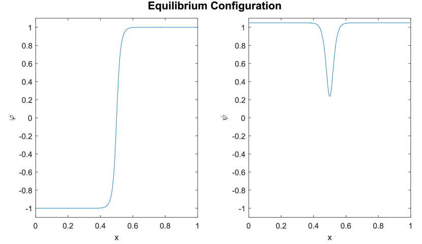
(c)                                                                                                                      (d)

Figure 5: Initial and equilibrium configuration of the ternary system with absent third phase in case of dynamically inconsistent coefficients.

mobility coefficients) is by introducing degenerate mobility, which is used and studied in binary phase field systems [15, 13, 11, 30, 39]. A similar approach can be used for degenerate models. However, it is interesting to make dynamic consistency energetically preferable as opposed to restricting the dynamics of the system through mobility.

Let us consider surface tension coefficients defined by

$$\gamma_{1}\left(\psi\right) =\frac{3}{2\sqrt{2}}\sigma_{12}\left(\frac{\psi+1}{2}\right)^{2},$$ (13)

$$\gamma_{2}\left(\varphi\right) =\frac{3}{2\sqrt{2}}\sigma_{13}=\frac{3}{2\sqrt{2}}\sigma_{23}=\mathrm{const},$$ (14)

where $\sigma_{12},\ \sigma_{13}$ and $\sigma_{23}$ are the surface tension constants on the corresponding interfaces. And to study the algebraic consistency we take an initial configuration with the third phase absent (see Fig. 5a,b). The Cahn-Hilliard equation describes the volume preserving minimization of the energy. Thus since the mixing energy in $\varphi$ is positive, by decreasing the value of $\gamma_{1}\left(\psi\right)$ and simultaneously increasing the $\psi$ portion of the mixing energy $\left(\frac{\varepsilon}{2}\left|\nabla\psi\right|^{2}+\frac{1}{4\varepsilon}\left(1-\psi^{2}\right)^{2}\right)$ the system can achieve a lower value of total energy.

This dynamics results in unnatural nucleation of the third phase, as in the case of the equilibrium configuration shown on figure 5c,d. In addition to the unnatural nucleation this behavior results in the decrease in equilibrium interfacial energy (comparing to the analytical assumption equal to surface tension multiplied by area of the interface). Numerical simulations show that this result does not depend on numerical precision, and decreasing interfacial thickness $\varepsilon$ results in a decrease in width of the cusp, but nearly does not affect height of the cusp and the energy loss.

As one can see from figure 6, both cusp size and relative energy loss increase with the ratio between surface tensions. Here, relative energy loss at the equilibrium is computed using the formula $\left|\sigma_{12}-\mathcal{W}\right|/\sigma_{12}.$

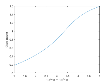
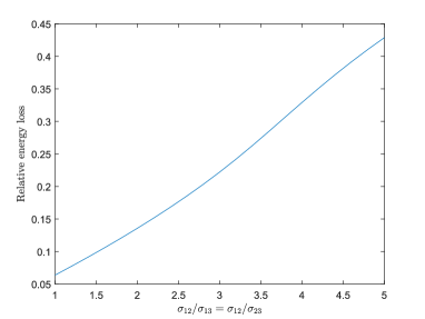
(a)	(b)

Figure 6: For the case of algebraically inconsistent coefficients (a) cusp height and (b) relative interfacial energy loss as a function of surface tension ratio.

To remedy this behavior all the coefficients in the energy need to have critical points at $\varphi=\pm 1$ and $\psi=\pm 1$. Additionally, to make this effect dynamically consistent (i.e. numerically stable, there should be no nucleation if the phase field is sufficiently close to $\pm 1$), one should require the coefficients to have double well structure, similar to that in the mixing energy. In particular, for $\gamma_{1}\left(\psi\right)$ and $\gamma_{2}\left(\varphi\right)$ we suggest the following formulation:

$$\gamma_{1}\left(\psi\right) =\frac{3}{2\sqrt{2}}\sigma_{12}\left(\frac{1+\psi}{2}\right)^{2}\left(2-\psi+\frac{\alpha}{4}\left(1-\psi\right)^{2}\right),$$ (15)

$$\gamma_{2}\left(\varphi\right) =\frac{3}{2\sqrt{2}}\left(\sigma_{13}\left(\frac{1+\varphi}{2}\right)^{2}\left(2-\varphi\right)+\sigma_{23}\left(\frac{1-\varphi}{2}\right)^{2}\left(2+\varphi\right)\right.$$

$$\qquad\quad\left.+\frac{\alpha}{16}\left|\sigma_{23}-\sigma_{13}\right|\left(1-\varphi^{2}\right){}^{2}\right).$$ (16)

Here $\alpha>3$ is a constant regulating the size of the double-well. One can take $\alpha=3+\varepsilon$ to reduce additional energy introduced by the double well structure of these terms at the triple junction. With $\alpha=3$ one would get fourth order interpolation in the interval $(-1,\,1)$ and convexity outside this interval.

Remark 1.

When $\alpha=3+\varepsilon$, the polynomial $\gamma_{2}\left(\varphi\right)$ satisfies the following conditions:

$$\gamma_{2}\left(1\right)=\frac{3}{2\sqrt{2}}\sigma_{13},\ \gamma_{2}\left(-1\right)=\frac{3}{2\sqrt{2}}\sigma_{23},\ \gamma_{2}^{\prime}\left(\pm 1\right)=0,\ \gamma_{2}^{\prime\prime}\left(\pm 1\right)>0,$$

$$\underset{-1<\varphi<1}{\max}\gamma_{2}\left(\varphi\right)=\frac{3}{2\sqrt{2}}\max\left(\sigma_{13},\,\sigma_{23}\right)+\frac{3}{2\sqrt{2}}\frac{\left|\sigma_{23}-\sigma_{13}\right|}{108}\varepsilon^{3}+O\left(\varepsilon^{4}\right).$$

Additionally, in case $\sigma_{13}=\sigma_{23}$ we obtain $\gamma_{2}\left(\varphi\right)=\frac{3\varepsilon}{2\sqrt{2}}\sigma_{13}=\mathrm{const}$.

Remark 2.

One should consider same kind of coefficients when introducing the additional (possibly non-Newtonian) structure into one of the components in binary model, so that changes in the structure inside the component do not affect the behavior of the phase field.

Remark 3.

Surface tension coefficients have to be interpolated only between two components. To interpolate a parameter $b_{\alpha}\left(\varphi,\,\psi\right)$ between all three components with values $b_{1},\ b_{2}$ and $b_{3}$ in the corresponding component, one may use a more complicated formula:

$$\begin{array}[]{rl}b_{\alpha}\left(\varphi,\psi\right)=&\left(b_{1}\left(\frac{1-\varphi}{2}\right)^{2}\left(2+\varphi\right)+b_{2}\left(\frac{1+\varphi}{2}\right)^{2}\left(2-\varphi\right)\right)\left(\frac{1+\psi}{2}\right)^{2}\left(2-\psi\right)\\ &+b_{3}\left(\frac{1-\psi}{2}\right)^{2}\left(2+\psi\right)+\frac{\alpha}{16}\left|b_{2}-b_{1}\right|\left(1-\varphi^{2}\right)^{2}\left(\frac{1+\psi}{2}\right)^{2}\left(2-\psi\right)\\ &+\frac{\alpha}{16}\left(\left|b_{3}-b_{1}\right|\left(\frac{1-\varphi}{2}\right)^{2}\left(2+\varphi\right)+\left|b_{3}-b_{2}\right|\left(\frac{1+\varphi}{2}\right)^{2}\left(2-\varphi\right)\right)\left(1-\psi^{2}\right)^{2}\\ &+\frac{\alpha^{2}}{16^{2}}\left|\left|b_{3}-b_{1}\right|-\left|b_{3}-b_{2}\right|\right|\left(1-\varphi^{2}\right)^{2}\left(1-\psi^{2}\right)^{2}\par\end{array}$$

3.2 Approach comparison

For two-phase systems there is a lot of research using order parameters both on intervals $(0,1)$ and $(-1,1)$. While those approaches are equivalent in case of binary mixture (which can be shown by linear change of variables), the difference in the dynamics of degenerate and non-degenerate ternary systems is fundamental – there is no linear relation connecting the models.

Let us introduce a non-linear change of variables:

$$c=\frac{1+\varphi}{2}\cdot\frac{1+\psi}{2},\quad d=\frac{1-\varphi}{2}\cdot\frac{1+\psi}{2}.$$ (17)

Substituting this into the mixing energy (7) we get

$$\frac{8}{3}\mathcal{W}=\int_{\Omega} \frac{\varepsilon}{2}\left(\sigma_{12}\left(\frac{1+\psi}{2}\right)^{2}\left|\nabla\varphi\right|^{2}+\frac{\sigma_{13}\left(1+\varphi\right)+\sigma_{23}\left(1-\varphi\right)-\frac{1}{2}\sigma_{12}\left(1-\varphi^{2}\right)}{2}\left|\nabla\psi\right|^{2}\right)$$

$$+\frac{\varepsilon}{2}\left(\sigma_{12}\varphi+\sigma_{13}-\sigma_{23}\right)\left(\frac{1+\psi}{2}\right)\left\langle\nabla\varphi,\,\nabla\psi\right\rangle+\frac{32}{\varepsilon}F\left(\varphi,\,\psi\right)d\mathbf{x}.$$ (18)

A natural extension of 2-phase potential $F$ within this framework is

$$F\left(c,\,d\right)= \sigma_{12}c^{2}d^{2}+\left(1-c-d\right)^{2}\left(\sigma_{13}c^{2}+\sigma_{23}d^{2}\right)$$

$$= \frac{1}{16}\left[\sigma_{12}\left(\frac{1+\psi}{2}\right)^{4}\left(1-\varphi^{2}\right)^{2}+\frac{\sigma_{13}\left(1+\varphi\right)^{2}+\sigma_{23}\left(1-\varphi\right)^{2}}{4}\left(1-\psi^{2}\right)^{2}\right].$$ (19)

The improved, algebraically and dynamically consistent version is then

$$F\left(c,\,d\right)= \sigma_{12}c^{2}d^{2}+\left(1-c-d\right)^{2}\left(\sigma_{13}c^{2}+\sigma_{23}d^{2}\right)$$

$$+cd\left(1-c-d\right)\left[\Sigma_{1}c+\Sigma_{2}d+\Sigma_{3}\left(1-c-d\right)\right]+\Lambda c^{2}d^{2}\left(1-c-d\right)^{2}=$$

$$= \frac{1}{16}\sigma_{12}\left(\frac{1+\psi}{2}\right)^{2}\left(1-\varphi^{2}\right)^{2}$$

$$+\frac{\sigma_{13}\left(1+\varphi\right)+\sigma_{23}\left(1-\varphi\right)-\frac{1}{2}\sigma_{12}\left(1-\varphi^{2}\right)}{32}\left(1-\psi^{2}\right)^{2}$$

$$+\frac{1}{16}\left(1-\varphi^{2}\right)\left(1-\psi^{2}\right)\left(\frac{1+\psi}{2}\right)^{2}\left[\sigma_{12}+\left(\sigma_{13}-\sigma_{23}\right)\varphi\right]$$

$$-\frac{1}{64}\sigma_{12}\left(1-\psi^{2}\right)\left(\frac{1+\psi}{2}\right)\left(\frac{3+\psi}{2}\right)\left(1-\varphi^{2}\right)^{2}$$

$$+\frac{1}{256}\Lambda\left(\frac{1+\psi}{2}\right)^{2}\left(1-\varphi^{2}\right)^{2}\left(1-\psi^{2}\right)^{2}.$$ (20)

Let us compare the resulting energy (18), (20) to the degenerate energy (10). Apart from a constant multiple, balance between diffusive and nonlinear terms, and $\gamma_{1}=\sigma_{12}\left(\frac{1+\psi}{2}\right)^{2}$ and $\gamma_{2}=\frac{\sigma_{13}\left(1+\varphi\right)+\sigma_{23}\left(1-\varphi\right)-\frac{1}{2}\sigma_{12}\left(1-\varphi^{2}\right)}{2}$ potentially leading to a dynamically inconsistent system, the differences are as follows:

• Cross-difusion term $\left(\sigma_{12}\varphi+\sigma_{13}-\sigma_{23}\right)\left(\frac{1+\psi}{2}\right)\left\langle\nabla\varphi,\,\nabla\psi\right\rangle$,

• Higher order nonlinear energy on the triple junction only

  $$\begin{array}[]{l}\frac{2}{\varepsilon^{2}}\left(1-\varphi^{2}\right)\left(1-\psi^{2}\right)\left(\frac{1+\psi}{2}\right)^{2}\left[\sigma_{12}+\left(\sigma_{13}-\sigma_{23}\right)\varphi\right]\\ -\frac{1}{2\varepsilon^{2}}\sigma_{12}\left(1-\psi^{2}\right)\left(\frac{1+\psi}{2}\right)\left(\frac{3+\psi}{2}\right)\left(1-\varphi^{2}\right)^{2}+\frac{1}{8\varepsilon^{2}}\Lambda\left(\frac{1+\psi}{2}\right)^{2}\left(1-\varphi^{2}\right)^{2}\left(1-\psi^{2}\right)^{2}.\end{array}$$

Overall, these differences may need to be considered in a more general terms to obtain the most physically relevant models.

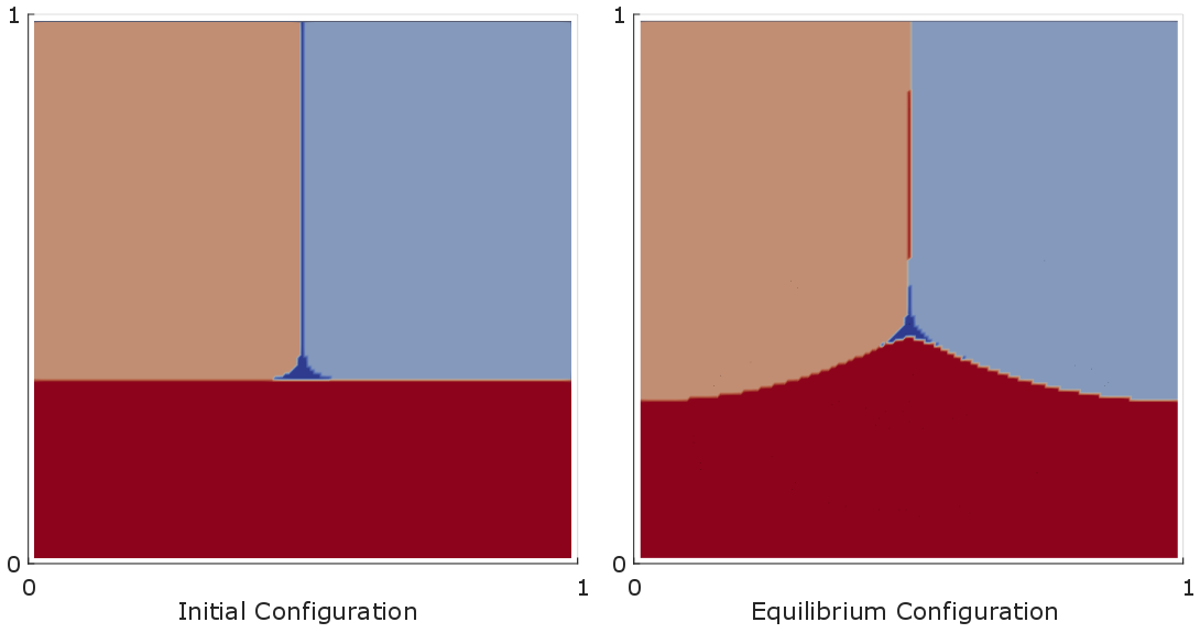
Figure 7: Initial configuration and equilibrium configuration of a three-component mixture.

Let us compare the dynamic behavior of the described systems on the example with initial and equilibrium states shown on figure 7. Here we take equal surface tensions $\sigma_{12}=\sigma_{13}=\sigma_{23}=1$.

First we look at the difference between the dynamics of the model derived from the non-degenerate mixing energy (7) vs the model derived from the same mixing energy rewritten in terms of variable $\varphi$ and $\psi$ given by formula (18), (20) (matching energy). Note that the latter system is not dynamically consistent, so under certain set of parameters may produce significant difference. As we can see from the figure 8a,b, the $L_{2}$ norm of the differences between relative concentrations is of order $10^{-4}$ and relative difference in energy stays bellow $2\cdot 10^{-3}$. This shows that behavior of the systems is nearly identical in this example.

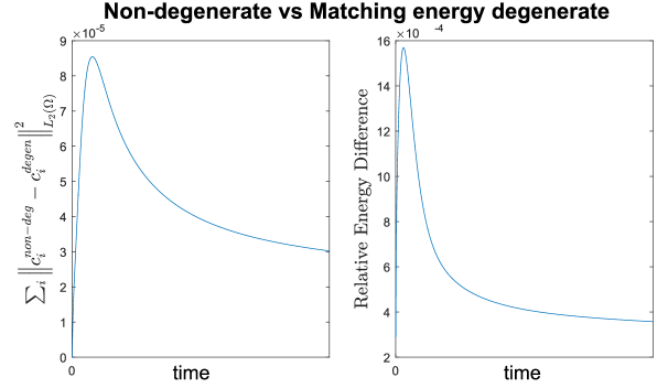
(a)                                               (b)

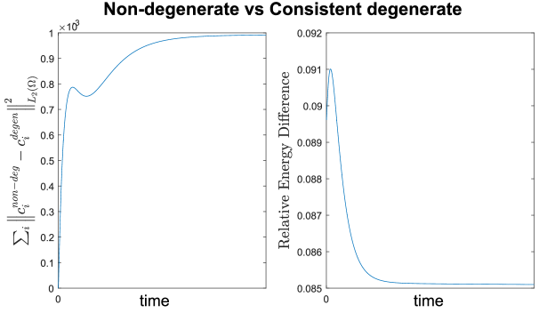
(c)                                                 (d)

Figure 8: Qualitative numerical comparison of the degenerate and non-degenerate models: (a, b) non-degenerate model vs degenerate model with matching energy; (c, d) non-degenerate model vs dynamically consistent degenerate model

Now on the same example we compare the two dynamically consistent models. Figure 8c,d demonstrates that the difference in concentrations remains qualitatively negligible, while the difference in the energy is more noticeable. This can be explained by the fact that the mixing energies under consideration approximate the surface tension differently. However, with $\varepsilon\rightarrow 0$ both converge to the desired value.

4 Conclusion

In this paper we analyze the consistency of the degenerate approach to diffusive interface modeling of ternary mixtures of immiscible fluids. The analysis results in a restriction on the way physical parameters are interpolated within the interface, which results in algebraic and dynamic consistency of the model with no restrictions on physical parameters. This model can be naturally extended to any number of components, while preserving the consistency. Moreover, we argue that the restrictions suggested should be applied to any diffusive interface model of immiscible mixture, where a physical property or parameter is interpolated within the interface.

We also perform a comparison of the degenerate approach to an earlier proposed non-degenerate approach. We have shown that the models have equivalence in the mixing energies used and behave qualitatively similar. One of the main differences is that nondegenerate model has restrictions on physical parameters it can be applied to. While having no physical restrictions, degenerate model has a more complicated nonlinear coefficients and approximates the immiscibility to the order of $\varepsilon$.

The future work includes design of stable numerical schemes for the degenerate model as well as consistently introducing non-newtonian effects in ternary mixtures.

Acknowledgments  The work of Arkadz Kirshtein and Chun Liu is partially supported by NSF grant DMS-1759536. The work of Arkadz Kirshtein and James Brannick is partially supported by NSF grant DMS-1620346.

Arkadz Kirshtein, Department of Mathematics, Pennsylvania State University, University Park, Pennsylvania 16802, USA

E-mail address, Arkadz Kirshtein: azk194@psu.edu

James Brannick, Department of Mathematics, Pennsylvania State University, University Park, Pennsylvania 16802, USA

E-mail address, James Brannick: brannick@psu.edu

Chun Liu, Department of Applied Mathematics, Illinois Institute of Technology, Chicago, IL 60616, USA

E-mail address, Chun Liu: cliu124@iit.edu

References

- [1] R. Abraham and J. E. Marsden. Foundations of mechanics. Benjamin/Cummings Publishing Company Reading, Massachusetts, 1978.
- [2] D. Anderson and G. B. McFadden. A diffuse-interface description of internal waves in a near-critical fluid. Physics of Fluids (1994-present), 9(7):1870–1879, 1997.
- [3] V. I. Arnol’d. Mathematical methods of classical mechanics, volume 60. Springer, 1989.
- [4] V. Berdichevsky. Variational Principles of Continuum Mechanics: I. Fundamentals. Springer Science & Business Media, 2009.
- [5] F. Boyer. A theoretical and numerical model for the study of incompressible mixture flows. Computers & fluids, 31(1):41–68, 2002.
- [6] F. Boyer and C. Lapuerta. Study of a three component Cahn-Hilliard flow model. ESAIM: Mathematical Modelling and Numerical Analysis, 40(04):653–687, 2006.
- [7] J. Brannick, A. Kirshtein, and C. Liu. Dynamics of multi-component flows: diffusive interface methods with energetic variational approaches. In S. Hashmi and M. Buggy, editors, Reference Module in Materials Science and Materials Engineering, pages 1–7. Elsevier, Oxford, 2016.
- [8] J. Brannick, C. Liu, T. Qian, and H. Sun. Diffuse Interface Methods for Multiple Phase Materials: An Energetic Variational Approach. Numerical Mathematics: Theory, Methods and Applications, 8(02):220–236, 2015.
- [9] J. Cahn and S. Allen. A microscopic theory for domain wall motion and its experimental verification in Fe-Al alloy domain growth kinetics. Le Journal de Physique Colloques, 38(C7):C7–51, 1977.
- [10] J. W. Cahn and J. E. Hilliard. Free energy of a nonuniform system. I. Interfacial free energy. The Journal of chemical physics, 28(2):258–267, 1958.
- [11] H. D. Ceniceros and C. J. García-Cervera. A new approach for the numerical solution of diffusion equations with variable and degenerate mobility. Journal of Computational Physics, 246:1–10, 2013.
- [12] Y.-C. Chang, T. Hou, B. Merriman, and S. Osher. A level set formulation of Eulerian interface capturing methods for incompressible fluid flows. Journal of computational Physics, 124(2):449–464, 1996.
- [13] Z. Chen. Degenerate two-phase incompressible flow: I. existence, uniqueness and regularity of a weak solution. Journal of Differential Equations, 171(2):203–232, 2001.
- [14] S. Dong. Wall-bounded multiphase flows of N immiscible incompressible fluids: Consistency and contact-angle boundary condition. Journal of Computational Physics, 338:21–67, 2017.
- [15] C. M. Elliott and H. Garcke. On the Cahn-Hilliard equation with degenerate mobility. SIAM Journal on Mathematical Analysis, 27(2):404–423, 1996.
- [16] C. M. Elliott and S. Luckhaus. A generalised diffusion equation for phase separation of a multi-component mixture with interfacial free energy’. Retrieved from the University of Minnesota Digital Conservancy,, 1991.
- [17] D. J. Eyre. Systems of Cahn-Hilliard equations. SIAM Journal on Applied Mathematics, 53(6):1686–1712, 1993.
- [18] H. Garcke, B. Nestler, and B. Stoth. On anisotropic order parameter models for multi-phase systems and their sharp interface limits. Physica D: Nonlinear Phenomena, 115(1):87–108, 1998.
- [19] M.-H. Giga, A. Kirshtein, and C. Liu. Variational Modeling and Complex Fluids. In Y. Giga and A. Novotny, editors, Handbook of Mathematical Analysis in Mechanics of Viscous Fluids, pages 1–41. Springer International Publishing, Cham, 2017.
- [20] M. E. Gurtin. Thermomechanics of evolving phase boundaries in the plane, volume 1. Oxford University Press, 1993.
- [21] M. E. Gurtin, D. Polignone, and J. Vinals. Two-phase binary fluids and immiscible fluids described by an order parameter. Mathematical Models and Methods in Applied Sciences, 6(06):815–831, 1996.
- [22] Y. Hyon, D. Y. Kwak, and C. Liu. Energetic variational approach in complex fluids: maximum dissipation principle. DCDS-A, 24(4):1291–1304, 2010.
- [23] D. Joseph. Fluid dynamics of two miscible liquids with diffusion and gradient stresses. European journal of mechanics. B, Fluids, 9(6):565–596, 1990.
- [24] D. D. Joseph and Y. Renardy. Fundamentals of Two-Fluid Dynamics. Part I: Mathematical Theory and Applications, volume 3 of Interdisciplinary Applied Mathematics. Springer-Verlag, New York, 1993.
- [25] D. D. Joseph and Y. Renardy. Fundamentals of Two-Fluid Dynamics. Part II: Lubricated Transport, Drops and Miscible Liquids, volume 4 of Interdisciplinary Applied Mathematics. Springer-Verlag, New York, 1993.
- [26] J. Kim, K. Kang, and J. Lowengrub. Conservative multigrid methods for Cahn-Hilliard fluids. Journal of Computational Physics, 193(2):511–543, 2004.
- [27] J. Kim, K. Kang, J. Lowengrub, and others. Conservative multigrid methods for ternary Cahn-Hilliard systems. Communications in Mathematical Sciences, 2(1):53–77, 2004.
- [28] J. Kim and J. Lowengrub. Phase field modeling and simulation of three-phase flows. Interfaces and free boundaries, 7(4):435, 2005.
- [29] R. Kubo. The fluctuation-dissipation theorem. Reports on progress in physics, 29(1):255, 1966.
- [30] A. A. Lee, A. Münch, and E. Süli. Degenerate mobilities in phase field models are insufficient to capture surface diffusion. Applied Physics Letters, 107(8):081603, 2015.
- [31] C. Liu and J. Shen. A phase field model for the mixture of two incompressible fluids and its approximation by a Fourier-spectral method. Physica D: Nonlinear Phenomena, 179(3):211–228, 2003.
- [32] C. Liu and N. J. Walkington. An Eulerian description of fluids containing visco-elastic particles. Archive for rational mechanics and analysis, 159(3):229–252, 2001.
- [33] J. Lowengrub and L. Truskinovsky. Quasi-incompressible Cahn-Hilliard fluids and topological transitions. Proceedings of the Royal Society of London. Series A: Mathematical, Physical and Engineering Sciences, 454(1978):2617–2654, 1998.
- [34] J. Morral and J. Cahn. Spinodal decomposition in ternary systems. Acta metallurgica, 19(10):1037–1045, 1971.
- [35] L. Onsager. Reciprocal relations in irreversible processes. I. Physical Review, 37(4):405, 1931.
- [36] L. Onsager. Reciprocal relations in irreversible processes. II. Physical Review, 38(12):2265, 1931.
- [37] T. Qian, X.-P. Wang, and P. Sheng. Molecular scale contact line hydrodynamics of immiscible flows. Physical Review E, 68(1):016306, 2003.
- [38] L. Rayleigh. Some general theorems relating to vibrations. Proceedings of the London Mathematical Society, 1(1):357–368, 1871.
- [39] A. Voigt. Comment on “Degenerate mobilities in phase field models are insufficient to capture surface diffusion” [Appl. Phys. Lett. 107, 081603 (2015)]. Applied Physics Letters, 108(3):036101, 2016.
- [40] P. Yue, J. J. Feng, C. Liu, and J. Shen. A diffuse-interface method for simulating two-phase flows of complex fluids. Journal of Fluid Mechanics, 515:293–317, 2004.
- [41] Q. Zhang and X.-P. Wang. Phase field modeling and simulation of three-phase flow on solid surfaces. Journal of Computational Physics, 319:79–107, 2016.