Torques on low-mass bodies in retrograde orbit in gaseous disks

Abstract

We evaluate the torque acting on a gravitational perturber on a retrograde circular orbit in the midplane of a gaseous disk. We assume that the mass of this satellite is so low it weakly disturbs the disk (type I migration). The perturber may represent the companion of a binary system with a small mass ratio. We compare the results of hydrodynamical simulations with analytic predictions. Our two-dimensional (2D) simulations indicate that the torque acting on a perturber with softening radius $R_{\rm soft}$ can be accounted for by a scattering approach if $R_{\rm soft}<0.3H$, where $H$ is defined as the ratio between the sound speed and the angular velocity at the orbital radius of the perturber. For $R_{\rm soft}>0.3H$, the torque may present large and persistent oscillations, but the resultant time-averaged torque decreases rapidly with increasing $R_{\rm soft}/H$, in agreement with previous analytical studies. We then focus on the torque acting on small-size perturbers embedded in full three-dimensional (3D) disks and argue that the density waves propagating at distances $\lesssim H$ from the perturber contribute significantly to the torque because they transport angular momentum. We find a good agreement between the torque found in 3D simulations and analytical estimates based on ballistic orbits. We compare the radial migration timescales of prograde versus retrograde perturbers. For a certain range of the perturber’s mass and aspect ratio of the disk, the radial migration timescale in the retrograde case may be appreciably shorter than in the prograde case. We also provide the smoothing length required in 2D simulations in order to account for 3D effects.

1. Introduction

Black hole (BH) binaries in the centers of galaxies may lose orbital angular momentum as a result of the gravitational interaction with the surrounding gas and stars (e.g., Ivanov et al., 1999; Milosavljević & Merritt, 2001; Armitage & Natarajan, 2002; Escala et al., 2004; Cuadra et al., 2009; Tanaka & Haiman, 2009; Kocsis, Haiman & Loeb, 2012; Mayer, 2013), which leads to a reduction of the separation between the BHs. In merging galaxies, the strong gas inflows may induce the formation of a circumbinary rotating disk. Tidal torques between the binary and the circumbinary disk may play an important role in the orbital evolution of the binary.

In the center of galaxies, BH binaries do not necessarily corotate with the disk because the angular momentum of new material accreted into the circumbinary disk may have a different (random) direction. Nixon et al. (2011) suggest that retrograde flows are as likely as prograde (see also Nixon, 2012; Miller & Krolik, 2013). Interestingly, Nixon et al. (2011) find that for retrograde binaries with mass ratios $\geq 0.1$, mass capturing into the secondary BH near apocenter leads to a rapid decrease in the orbital angular momentum of the binary while only a modest change in its orbital energy; the eccentricity of the binary grows and the pericenter distance is shortened. This reduction of the pericenter distance may bring the BHs close enough for gravitational wave radiation to drive their merger.

A number of papers have studied the evolution of the orbital parameters of a binary surrounded by a retrograde accretion disk using numerical simulations (e.g., Roedig & Sesana, 2014; Bankert, Krolik & Shi, 2015; Nixon & Lubow, 2015; Amaro-Seoane et al., 2016). All the abovementioned papers consider the non-linear regime, that is, they adopt secondary to primary mass ratios $q$ between $0.1$ and $1$.

On the other hand, Ivanov et al. (2015) study a binary with small $q$ immersed in a retrograde disk through semi-analytic methods and two-dimensional (2D) simulations. They mainly focus on binary mass ratios that are small but large enough to significantly perturb the disk.

Here we study the accretion and gravitational torques acting on a retrograde satellite with such a small mass that it is unable to carve a gap or open a cavity in the disk. In the context of planetary migration, this regime is referred to as type I migration. The perturbing mass may represent the secondary component of a binary with small mass ratio, or a stellar cluster or dwarf galaxy embedded in a gas-rich host galaxy. In this paper, we will mainly talk about binary systems, but the majority of our results can be translated to galactic systems.

Binary systems consisting of two BHs and having small values of $q$ can arise in the core of the merger of unequal-mass galaxies (e.g., Khan et al., 2012). They can also arise in systems composed by a supermassive BH and a stellar-mass BH (or star) trapped in the accretion disk (e.g., Bartos et al., 2017), or in systems composed by a supermassive BH and an intermediate-mass BH. In fact, it has been suggested that intermediate-mass BHs can grow efficiently in disks around supermassive BHs via mass accretion (McKernan et al., 2012).

The paper is organized as follows. A short overview of the assumptions together with some definitions are given in Section 2. In Section 3, we compile the different analytical estimates of the gravitational torque acting on a retrograde satellite embedded in a gaseous disk. In Section 4, these analytical estimates are compared to the results based on hydrodynamical simulations. Some implications of our results are presented in Section 5. Our conclusions are given in Section 6.

2. Basic assumptions and relevant parameters

Consider a rotating disk with surface density $\Sigma(\mbox{\boldmath$r$}{},t)$ in a spherical background potential $\Phi_{b}$. Suppose that a small satellite (perturber) of mass $M_{2}$ is on a fixed circular orbit with radius $a_{2}$. The mass within a sphere of radius $a_{2}$ is $M_{1}$. The ratio between these masses, $q\equiv M_{2}/M_{1}$, is assumed to be small. Therefore, the perturber rotates with angular velocity $\omega\equiv\sqrt{GM_{1}/a_{2}^{3}}$. In the particular case of a binary, $M_{1}$ and $M_{2}$ are the masses of the primary and the secondary, respectively. Note that by assumption, the disk’s mass is negligible compared to $M_{1}$.

We assume that the interaction between the perturber and the disk is exclusively gravitational; the perturber does not have any rigid surface. The gravitational potential associated with the perturber is given by

$$\Phi_{2}(\mbox{\boldmath$r$}{},t)=-\frac{GM_{2}}{\sqrt{|\mbox{\boldmath$r$}{}-\mbox{\boldmath$r$}{}_{2}|^{2}+R_{\rm soft}^{2}}},$$ (1)

where $\mbox{\boldmath$r$}{}_{2}(t)$ is the position of the perturber and $R_{\rm soft}$ is a softening radius, which is nonzero for finite-sized bodies and it is zero for point-mass accretors. The exchange of angular momentum with the disk through waves produces a dynamical torque on the perturber. In addition to this dynamical torque, and for point-like satellites ($R_{\rm soft}=0$), accretion of material may lead to an “aerodynamic” drag.

For systems with a mass ratio $q$ well below a certain critical value $q_{\rm cr}$, the torques expressed on the disk are too small to significantly alter its density structure (type I migration). However, for $q\gtrsim q_{\rm cr}$, the torques can open an annular gap in the surface density of the disk at the location of the perturber (type II migration).

In the prograde case, $q_{\rm cr}$ is given by

$$q_{\rm cr}^{(p)}=10\left(\frac{\nu}{\omega a_{2}^{2}}\right)^{1/2}h^{3/2}=10\sqrt{\alpha}h^{5/2},$$ (2)

where $\nu$ is the viscosity of the disk, $\alpha$ is the Shakura-Sunyaev viscosity parameter and $h$ is the disk’s aspect ratio $h\equiv H/a_{2}$ (e.g., Lin & Papaloizou, 1986; Chametla et al., 2017). Here $H$ is the vertical scaleheight of the disk at the perturber’s location. Along the paper, we will use the scripts $(p)$ and $(r)$ to distinguish between the prograde case and the retrograde case.

In the retrograde case and assuming that the perturbing particle is a perfect accretor, such as a BH or a star, $q_{\rm cr}^{(r)}$ can be obtained by imposing that its mass accretion rate must be smaller than the radial flow rate of mass in the disk. For a Keplerian disk with viscosity $\nu$, the radial mass flow is $3\pi\nu\Sigma$, while the accretion rate by the perturber is $\pi\rho R_{\rm acc}^{2}V_{\rm rel}$, where $\rho$ is the disk’s density at the cylindrical radius $a_{2}$, $V_{\rm rel}$ is the relative velocity of the perturber with respect to the gas and $R_{\rm acc}\equiv 2GM_{2}/V_{\rm rel}^{2}$ is the accretion radius. In the retrograde case, $V_{\rm rel}=2\omega a_{2}$ and $R_{\rm acc}=qa_{2}/2$. For the density, we take $\rho=\Sigma/(\sqrt{2\pi}H)$, which corresponds to the midplane density of a Gaussian vertical profile. Hence, the type I condition implies

$$q<q_{\rm cr}^{(r)}\equiv 4\left(\frac{\nu}{\omega a_{2}^{2}}\right)^{1/2}h^{1/2}.$$ (3)

In terms of the Shakura-Sunyaev viscosity parameter $\alpha$, $q_{\rm cr}^{(r)}$ can be expressed as $q_{\rm cr}^{(r)}=4\alpha^{1/2}h^{3/2}$. The type I condition can be recast in terms of the accretion radius as

$$R_{\rm acc}\lesssim 2\left(\frac{\nu}{\omega a_{2}^{2}}\right)^{1/2}h^{1/2}a_{2}.$$ (4)

For a retrograde disk with parameters $h=0.05$ and $\nu=10^{-5}\omega a_{2}^{2}$, the type I condition is fulfilled as long as $q\lesssim q_{\rm cr}^{(r)}=2.8\times 10^{-3}$ or, equivalently, $R_{\rm acc}\lesssim 0.028H$.

Ivanov et al. (2015) evaluate the minimum value of $q$ for gap opening through tidal torques, instead of being the result of depletion by accretion. They establish that tidal torques are too weak to open a gap if $q\leq 1.57h^{2}$. This upper limit for $q$ coincides with our condition (3) for a disk with $h=0.05$ and $\nu=2\times 10^{-5}\omega a_{2}^{2}$. For lower viscosities or/and thicker disks, the condition given in Eq. (3) is more stringent.

Retrograde systems with $q$ larger than $q_{\rm cr}^{(r)}$ may still lie in the type I regime if the perturber is an extended body. In particular, the type I condition is met if $R_{\rm soft}\gg R_{\rm acc}$ because the response of the disk is linear at any location in this case (e.g., Bernal & Sánchez-Salcedo, 2013; Ivanov et al., 2015).

3. Torques in a retrograde disk

Without loss of generality, we take in both theoretical analysis and simulations throughout the paper, that the disk rotates in counterclockwise direction. For the retrograde case, the satellite rotates in the clockwise direction. We denote $dT_{g}/dR$ the torque acting upon an elementary ring of radius $R$ and width $\delta R$, and use the sign convention that the ring loses (gains) angular momentum if $dT_{g}/dR$ is negative (positive).

3.1. Strict 2D disk

A first estimate of the excitation torque density $dT_{g}/dR$ exerted by a retrograde satellite on a 2D disk can be obtained in the impulse approximation in a similar way as Lin & Papaloizou (1979, 1993) did for the prograde case. The impulse approximation yields

$$\frac{dT_{g}}{dR}\simeq-\frac{1}{2}q^{2}\Sigma a_{2}^{3}\omega^{2}\left(\frac{a_{2}}{R-a_{2}}\right)^{2}.$$ (5)

Ivanov et al. (2015) use that expression for the torque density to predict the density profile of the disk and the gap profile in the nonlinear case.

A more refined derivation of the excitation torque density can be done using perturbation analysis of the orbits (see Appendix). For a Keplerian disk, we find

$$\frac{dT_{g}}{dR}=-\frac{1}{8}q^{2}\Sigma\omega^{2}a_{2}^{3}\left(\frac{a_{2}}{R}\right)^{3}\left(-2K_{0}\left[\frac{\xi}{2R}\right]+\frac{\Delta}{\xi}K_{1}\left[\frac{\xi}{2R}\right]\right)^{2}$$ (6)

where $\Delta\equiv R-a_{2}$, $\xi=(\Delta^{2}+R_{\rm soft}^{2})^{1/2}$ and $K_{n}$ are the modified Bessel functions. For impact parameters such that $\xi\ll R$, Equation (6) can be approximated by

$$\frac{dT_{g}}{dR}\simeq-\left(\frac{1}{2}\right)q^{2}\Sigma\omega^{2}a_{2}^{3}\left[\frac{R\Delta}{\xi^{2}}+\ln\left(\frac{\xi}{4R}\right)+0.577\right]^{2}.$$ (7)

In general, the impulse approximation (Equation 5) overestimates (underestimates) the torque density in the external (internal) disk, as compared to Equation (7). Only in the particular case that $R_{\rm soft}\ll|\Delta|\leq 0.05a_{2}$, we can approximate the torque density by Equation (5) with an error $\lesssim 50\%$ in the external disk ($\Delta>0$) and $\lesssim 30\%$ in the internal disk ($\Delta<0$).

Figure 1.— Dimensionless torque as a function of the softening radius for $q=10^{-3}$ using the orbital scattering approach. The solid curve corresponds to the torque derived using Equations (6) and (8) with $\Delta_{1}=\Delta_{2}=0.2a_{2}$. The dotted and dashed lines are the torques derived using Equations (7) and (8) with $\Delta_{1}=\Delta_{2}=0.2a_{2}$ (dotted line) and with $\Delta_{1}=\Delta_{2}=0.5a_{2}$ (dashed line).

The net torque acting on the perturber, $T_{p}$, can be calculated by integrating $dT_{g}/dR$ over $R$ or, equivalently, over $\Delta$. Since our perturbation analysis is strictly valid only for $\xi\ll a_{2}$, which implies $\Delta\ll a_{2}$, we compute the net torque as

$$T_{p}=-\int_{-\Delta_{1}}^{\Delta_{2}}\frac{dT_{g}}{d\Delta}\,d\Delta,$$ (8)

where the integral limits $\Delta_{1}$ and $\Delta_{2}$ must be taken less than $a_{2}$. Note that the integration in Equation (8) diverges if $R_{\rm soft}=0$ and $\Delta\rightarrow 0$. The reason is that Equation (7) is not valid for small impact parameters if $R_{\rm soft}=0$. In fact, in the integration over $\Delta$, we have to exclude the streamlines that suffer significant deflection. The condition for small deflections is given in Eq. (A13) in the Appendix. For a point mass ($R_{\rm soft}=0$), it requires that the impact parameter $\Delta$ should be larger than $20R_{\rm acc}$.

Figure 1 shows $T_{p}$ as a function of $R_{\rm soft}$ for $q=10^{-3}$. We compute $T_{p}$ using Eqs. (6) and (8), for $\Delta_{1}=\Delta_{2}=0.2a_{2}$. For comparison we also plot the net torque derived using Equation (7) instead of Equation (6), for $\Delta_{1}=\Delta_{2}=0.2a_{2}$ and for $\Delta_{1}=\Delta_{2}=0.5a_{2}$. We see that the three curves almost overlap. The curves have an inflection point at $R_{\rm soft}\simeq 0.005a_{2}$. For values of $R_{\rm soft}$ smaller than $0.005a_{2}$, $T_{p}$ flattens because of the exclusion of those impact parameters that produce large deflections.

The scattering approach is usually adopted to estimate the torque density in the nonlinear type II regime. For perturbers with $q$ small enough that $R_{\rm acc}\ll R_{\rm soft}$, the response of the disk is linear even in the immediate vicinity of the perturber and thus the torque $T_{p}$ can be computed using linear theory. Muto et al. (2011) derived the linear dynamical friction force on a softened object moving in a rectilinear orbit with constant velocity $V_{\rm rel}$ through a 2D (zero thickness) slab of constant surface density $\Sigma$ and sound speed $c_{s}$. For a supersonic perturber, the dynamical friction force, according to Muto et al. (2011), is

$$F_{\rm\scriptscriptstyle DF}\simeq\frac{\pi\Sigma G^{2}M_{2}^{2}}{R_{\rm soft}V_{\rm rel}^{2}}.$$ (9)

Applying this formula to a body on a retrograde circular orbit and making use of the relations $GM_{2}=q\omega^{2}a_{2}^{3}$ and $V_{\rm rel}=2\omega a_{2}$, the torque is

$$T_{p}=a_{2}F_{\rm\scriptscriptstyle DF}=\frac{\pi}{4}q^{2}\Sigma\omega^{2}a_{2}^{4}\left(\frac{a_{2}}{R_{\rm soft}}\right).$$ (10)

In Figure 2, we see that the curve for $T_{p}$ derived in linear theory closely follows the curve derived in the scattering calculation.

As an alternative method, Ivanov et al. (2015) study the linear interaction between a retrograde circular-orbit satellite (secondary) and a 2D disk, by assuming that the flow is stationary in a frame rotating with the secondary. The torque $T_{p}$ is written as a summation of the contribution of the different Fourier modes with azimuthal wave number $m$. According to Ivanov et al. (2015), the torque in the linear regime is

$$T_{p}=2\pi q^{2}\Sigma\omega^{2}a_{2}^{4}\left(\frac{a_{2}}{H}\right)$$

$$\times\sum_{m=1}^{\infty}\frac{m}{\sqrt{4m^{2}-1}}\exp\left(-2\sqrt{4m^{2}-1}R_{\rm soft}/H\right),$$ (11)

where $H\equiv c_{s}/\omega$ with $c_{s}$ the sound speed evaluated at $R=a_{2}$. Equation (11) can be approximated by

$$T_{p} \simeq\frac{2\pi}{\sqrt{3}}q^{2}\Sigma\omega^{2}a_{2}^{4}\left(\frac{a_{2}}{H}\right)$$ (12)

$$\times\biggl{(}\exp\left[-\frac{2\sqrt{3}R_{\rm soft}}{H}\right]+\frac{2}{\sqrt{5}}\exp\left[-\frac{2\sqrt{5}R_{\rm soft}}{H}\right]$$

$$+\frac{\sqrt{3}}{2}\frac{\exp(-12R_{\rm soft}/H)}{1-\exp(-4R_{\rm soft}/H)}\biggl{)}.$$

If $R_{\rm soft}\ll 0.2H$, the last term in the right-hand side of Equation (12) is the leading term, and the expression (10) for the torque is recovered. Indeed, it easy to check that Equation (10) is a good approximation of Equation (12) for $R_{\rm soft}\leq 0.3H$ with a fractional error less than $16\%$. In this limit, the torque $T_{p}$ is essentially independent of $H$ (see Eq. 10).

Figure 2.— Dimensionless torque as a function of the softening radius using different approaches. The solid line is calculated after adopting Equations (6) and (8) with $\Delta_{1}=\Delta_{2}=0.2a_{2}$, the dotted lines using Equation (10), and the dashed lines correspond to Equation (12). In all cases it is assumed that $q$ is small enough that $R_{\rm acc}\ll R_{\rm soft}$.

For $R_{\rm soft}>0.3H$, the third term in the right-hand side of Equation (12) is small compared to the two first terms. Given $H$, Equation (12) then predicts that the torque declines exponentially when increasing $R_{\rm soft}$ with a characteristic scale $\sim H/4$. On the other hand, if $R_{\rm soft}$ is kept fixed, Equation (12) predicts that the magnitude of the torque is sensitive to the value of $H$. In particular, if $H\rightarrow 0$ (i.e. $c_{s}\rightarrow 0$), then $T_{p}\rightarrow 0$.

The above features are exemplified in Figure 2 where we compare $T_{p}$ versus $R_{\rm soft}$, under the different approaches. The values of the torque predicted by Equation (12) converge to the values derived in the scattering method only for small values of $R_{\rm soft}/H$. For values $R_{\rm soft}/H\gtrsim 1$, Equation (12) predicts smaller torques than the other two methods. For instance, for $R_{\rm soft}=0.04a_{2}$ and $H=0.025a_{2}$ (implying $R_{\rm soft}=1.6H$), Equation (12) predicts a torque about $30$ times lower than Equations (6) or (10).

The estimates of $T_{p}$ given in Eqs. (6) and (10) ignore the gravitational torque exerted by the perturbed disk at the front side of the satellite. If we drop the satellite at $t=0$ in an unperturbed disk, these estimates should be good at least at times $t\leq\tau_{1/2}$, that is, before the satellite has reached its own wake. At $t\gg\tau_{1/2}$, Equation (12) should be more precise as it takes into account the contribution of this material. Equations (6), (10) and (12) converge if $R_{\rm soft}\ll H$. The reason for this matching at large $H$ is that in thicker disks, the wake is less colimated when the perturber penetrates into it and hence the gravitational push is less important. In fact, the condition $R_{\rm soft}\ll H$ implies that the thickness of the wake, when the perturber reaches its tail (which is $c_{s}\tau_{1/2}$) is much larger than $R_{\rm soft}$.

In Section 4, we present the results of 2D simulations in order to answer the following questions: Does the torque take a value as predicted by Equations (6) and (10) at $t\simeq\tau_{\scriptscriptstyle 1/2}$? At later times, does the torque decrease with time to the value predicted by Equation (12)? If so, what is the timescale for this relaxation process?

3.2. Torques in a retrograde 3D disk

The 2D analysis is strictly valid only if the vertical velocity dispersion of the disk particles is zero and thus the disk has zero thickness at any time. 2D models correctly describe the far field (i.e. at distances from the perturber much larger than $H$), but a delicate vertical averaging procedure is necessary to obtain the 2D equations to account for the otherwise neglected vertical thickness of the disk (e.g., Müller et al., 2012; Kley et al., 2012).

In the context of type I migration, it was soon noticed that the 2D theory could give a reasonable estimate of the 3D torque in the prograde case, even if the perturber has a size much less than $H$ (e.g., §5.3 in Artymowicz 1993; Takeuchi & Miyama 1998). This is because of the existence of the torque cut-off: acoustic waves cannot be excited at a distance from the perturber less than $\sim H$ if the perturber is on a prograde orbit because the gas velocity relative to the perturber is subsonic and, in a stationary state, a subsonic perturber cannot excite acoustic waves. More quantitatively, Tanaka et al. (2002) computed the torque in linear theory for a 2D disk and for a 3D disk. In the particular case of a disk with constant surface density, the torque for the 3D case is only $18\%$ higher than it is for the 2D case.

However, if the secondary has a retrograde orbit, its relative velocity with respect to the gas is supersonic at any distance from the perturber. As a consequence, the perturber can excite acoustic waves at distances $\leq H$, especially if it is a point-mass with $R_{\rm acc}\ll H$. These waves carry angular momentum and contribute to the torque. Therefore, a 3D treatment of the interaction is required to evaluate the torque. The 3D analysis is also important if we wish to capture 3D effects in 2D simulations.

3.2.1 Analytical predictions

Cantó et al. (2013) use the ballistic approximation to compute the dynamical friction force on a gravitational perturber moving along a rectilinear trajectory, at relative velocity with respect to the gas $V_{\rm rel}$, in the midplane ($z=0$) of a vertically-stratified slab with density $\rho(z)=\rho_{0}\exp(-z^{2}/2H^{2})$.

For a perfect accretor ($R_{\rm soft}=0$) with $R_{\rm acc}\ll H$, Cantó et al. (2013) obtain that the drag force is

$$F_{\rm\scriptscriptstyle DF}=\frac{\sqrt{8\pi}\Sigma(GM_{2})^{2}}{V_{\rm rel}^{2}H}\ln\left(\left[\frac{8e^{3}}{\pi}\right]^{1/2}\frac{H}{R_{\rm acc}}\right),$$ (13)

where $\Sigma$ is the surface density of the slab ($\Sigma=\sqrt{2\pi}\rho_{0}H$). Using again that for a perturber in counter-rotating circular orbit $V_{\rm rel}=2\omega a_{2}$ and $GM_{2}=q\omega^{2}a_{2}^{3}$, the corresponding torque is

$$T_{\rm bal}^{(r)}=\sqrt{\frac{\pi}{2}}\frac{q^{2}}{h}\Sigma\omega^{2}a_{2}^{4}\ln\left(\frac{14.3h}{q}\right),$$ (14)

where we have used that $R_{\rm acc}=qa_{2}/2$. It is important to remark here that the aerodynamic torque due to mass accretion by the perturber, which is given by

$$T_{\rm acc}^{(r)}=\frac{\pi}{2}\frac{q^{2}}{h}\Sigma\omega^{2}a_{2}^{4},$$ (15)

has also been included in $T_{\rm bal}^{(r)}$. The aerodynamic torque $T_{\rm acc}^{(r)}$ is not negligible; for $h/q=50$, $T_{\rm acc}^{(r)}$ contributes $19\%$ to the total torque $T_{\rm bal}^{(r)}$.

For a non-accreting perturber with softening radius much smaller than $H$, Cantó et al. (2013) infer that

$$F_{\rm\scriptscriptstyle DF}=\frac{\sqrt{8\pi}\Sigma(GM_{2})^{2}}{V_{\rm rel}^{2}H}\ln\left(\frac{r_{\rm max}}{r_{\rm min}}\right),$$ (16)

where $r_{\rm max}\simeq 2.1\sqrt{2}H$ and $r_{\rm min}$ is the minimum impact parameter for the interaction. In the case of a Plummer perturber with $R_{\rm soft}>R_{\rm acc}$, Bernal & Sánchez-Salcedo (2013) found that $r_{\rm min}=2.25R_{\rm soft}$ (see also Sánchez-Salcedo & Brandenburg, 1999). Putting together, the predicted torque on a softened body having $R_{\rm acc}<R_{\rm soft}\ll H$, on a retrograde circular orbit, is

$$T_{\rm bal}^{(r)}=\sqrt{\frac{\pi}{2}}\frac{q^{2}}{h}\Sigma\omega^{2}a_{2}^{4}\ln\left(\frac{1.32H}{R_{\rm soft}}\right).$$ (17)

On the other hand, Ivanov et al. (2015) also give an expression for the torque on a small perturber ($R_{\rm acc}<H$ and $R_{\rm soft}<H$) using the linear mode decomposition. If the disturbing body is not very massive (more specifically, for $q$ less than $3\pi h/5$, which is the range of interest in the present investigation), they find

$$T_{\rm wave}^{(r)}=\frac{5}{3}\frac{q^{2}}{h}\Sigma\omega^{2}a_{2}^{4},$$ (18)

without distinction between accreting or non-accreting perturbers. Equation (18) is similar to Equations (14) and (17), except by factors of order unity and the logarithmic dependence. By comparing Eq. (15) and (18), we find that $T_{\rm wave}^{(r)}$ is only $6\%$ larger than $T_{\rm acc}^{(r)}$, which suggests that $T_{\rm wave}^{(r)}$ might underestimate the net torque on an accreting perturber. Moreover, $T_{\rm bal}^{(r)}$ may be significantly larger than $T_{\rm wave}^{(r)}$. For instance, for a perfect accretor ($R_{\rm soft}=0$) with $h/q$ between $50$ and $500$, $T_{\rm bal}^{(r)}$ is a factor of $5-7$ larger than $T_{\rm wave}^{(r)}$. In the next Section, we present the results of 3D simulations to test the accuracy of these two formulae.

4. Hydrodynamical simulations

We have carried out 2D and 3D simulations of a binary embedded in a gaseous disk, using the FARGO3D code (Benítez-Llambay & Masset, 2016). We use a spherical grid $(r,\phi,\theta)$. The self-gravity of the disk is not included. In all our simulations, the secondary with a mass $q=10^{-3}$ is dropped suddently at $t=0$ and it is held on a fixed circular orbit in retrograde direction. Initially, the disk has pure azimuthal rotation and constant surface density. The thermal profile is fixed by assuming that the ratio between the sound speed and the circular velocity is constant with $R$. The evolution is locally isothermal. The kinematical viscosity of the disk was taken $\nu=10^{-5}\omega a_{2}^{2}$ in all the simulations. We simulate a ring of the disk with inner radius $r_{\rm min}$ and outer radius $r_{\rm max}$. In the radial direction we employ damping boundary conditions at $r_{\rm min}$ and at $r_{\rm max}$ (de Val-Borro et al., 2006). Remind that the disk rotates in counterclockwise direction and the binary in clockwise direction: the secondary loses angular momentum if the torque $T_{p}$ is positive.

Two dimensionless parameters define a model: $h\equiv H/a_{2}=c_{s}/(\omega a_{2})$ and $s\equiv R_{\rm soft}/a_{2}$. In terms of $h$, a retrograde perturber in circular orbit travels at a Mach number ${\mathcal{M}}=2/h$ relative to the local gas.

We have checked that convergence of the results requires at least $2$ zones per $R_{\rm soft}$ in the radial direction, and $1.5$ zones per $R_{\rm soft}$ in the azimuthal and vertical directions.

4.1. 2D simulations

In all the simulations presented in this subsection, we use $r_{\rm min}=0.3a_{2}$ and $r_{\rm max}=4a_{2}$, and the number of zones per $R_{\rm soft}$ is taken to be larger than $2$ in each direction, in order to obtain reliable estimates of the torque. We have explored the effect of the finite size of the domain by comparing models at varying size of the domain (see Figure 3). In all these models, the number of zones per $R_{\rm soft}$ is $9$ in the radial direction and $1.5$ in the azimuthal direction and, therefore, all they have the same spatial resolution. We find that for $r_{\rm min}\lesssim 0.3a_{2}$ and $r_{\rm max}\gtrsim 3a_{2}$, the torque is estimated with reasonable accuracy. In fact, the torque for the model having $r_{\rm min}=0.2a_{2}$ and $r_{\rm max}=6a_{2}$ (not shown) overlaps with the curve obtained for $r_{\rm min}=0.25a_{2}$ and $r_{\rm max}=3.5a_{2}$.

Figure 3.— Dimensionless torque versus time, in 2D runs, for different values of $r_{\rm min}$ and $r_{\rm max}$ (in units of $a_{2}$), but having the same number of zones per $R_{\rm soft}$. In all cases, $h=0.06$ and $s=0.006$.

   

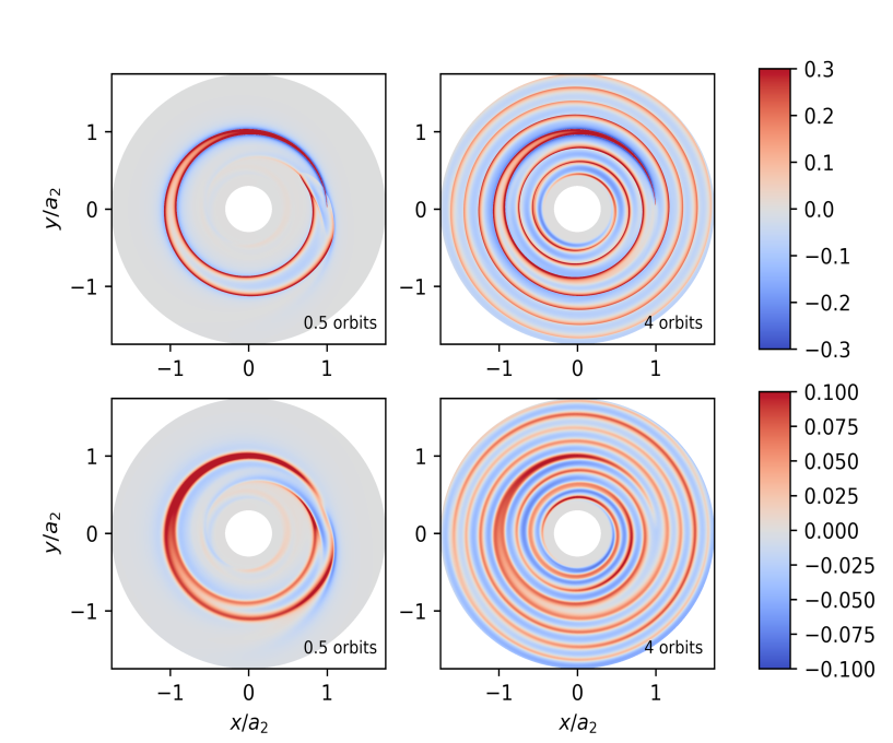
Figure 4.— Snapshots of the perturbation of the surface density $(\Sigma-\Sigma_{i})/\Sigma_{i}$, where $\Sigma_{i}$ is the initial surface density, in 2D runs with $h=0.05$ and $s=0.006$ (upper panels), and with $h=0.05$ and $s=0.06$ (lower panels). The time is quoted at the lower-right corner in each panel. The secondary is at $x/a_{2}=1$ and $y=0$ in all the panels. Only the central regions of the disk is shown (the computional domain extends up to $r_{\rm max}=4a_{2}$).

Figure 5.— Dimensionless torque as a function of time in 2D simulations with different combinations of $h$ and $s$ (see legends).

Our first objective is to find out the dependence of the strength of the torque with $R_{\rm soft}$ and with the gas sound speed (or, equivalently with $h$). To do so, we have computed the torque on the perturber for several values of $s$, spanning between $0.006$ and $0.06$, and different values of $h$, between $0.025$ and $0.15$.

Figure 4 displays color maps of the perturbed surface density for a disk with $h=0.05$ and two different softening radii ($s=0.006$ and $s=0.06$). The density wake consists of very thin plumes that are curved along the orbit. These plumes are bounded by sharp discontinuities. After a few orbits, the density wake becomes tighly wound.

Figure 6.— Comparison of the torque in 2D simulations (symbols) and analytical predictions (lines). The top panel shows $T_{p}^{\ast}$ for different simulated models, while the solid line indicates the torque using the ballistic approximation presented in §3. A small shift along the horizontal axis has been introduced to avoid overlapping. The middle panel shows $\left<T_{p}\right>$ versus $s$ for the same models. The dashed lines represent the curves using Equation (12), for varying values of $h$. The bottom panel shows $s\left<T_{p}\right>$ as a function of $R_{\rm soft}/H$. The dashed line corresponds to the curve predicted by Equation (12).

The behaviour of the torque versus time is shown in Figure 5 for seven representative cases. Consider first the magnitude of the torque at early stages, i.e. at $t<0.4$ orbits, when the perturber has not penetrated yet into its own wake. We see in this Figure that the torque at those times depends on $s$ but it is not sensitive to the disk aspect ratio $h$, i.e. it does not depend on the sound speed of the gas. This is in agreement with Equations (6) and (10). The reason is that the perturber moves so highly supersonic that the trajectory of a fluid element can be obtained by neglecting the pressure force. In this limit, the sound speed of the gas is not relevant in determining the torque. This pressureless approximation was already made by Bondi & Hoyle (1944) to study mass accretion onto a star. In order to check further whether or not the ballistic approximation developed in §3 reproduces satisfactorily the torque at early times, it is convenient to define $T_{p}^{\ast}$ as the mean torque between $t=0.05$ and $t=0.4$ orbits. The upper panel of Figure 6 compares $T_{p}^{\ast}$ as obtained from our simulationes with the torque predicted by Equations (6) and (8). We find a good agreement between them.

At $t\simeq 0.5$ orbits, the secondary encounters its own tail. At this time, in most of the cases, the torque exhibits a remarkable peak and then an abrupt decline. This is the result of the interaction with small-scale density substructures in the wake, as the secondary runs close to them (see Figure 4). Indeed, during the first $2.5$ orbits, the disk is at the process of relaxation and the torque may exhibit some narrow fluctuations until those density substructures are smeared out. Note, however, that these fluctuations in the torque are small for disks with $h=0.15$.

After $t\simeq 2.5$ orbits, the torque reaches a nearby constant value in the models with $h=0.15$. In these models, the wake achieves a quasi-stationary state in the frame rotating with the perturber. For a compact body (i.e. $s=0.006$), and a relatively hot disk ($h=0.15$), its stationary value is almost identical to $T_{p}^{\ast}$ (see first panel of Figure 5).

On the other hand, in models with $h\leq 0.05$, the torque oscillates around the mean value with frequency $\omega$. To be sure that these oscillations are not a numeric artefact, we varied the viscosity, the value of the mass of the secondary, and used different rotating frames of reference, as well as different initial radial profiles for the disk surface density. In all these variations, the oscillations in the torque are present. At a fixed value of $c_{s}$, say at $h=0.05$, the amplitude of these oscillations is rather insensitive to the adopted value of $s$. All this suggests that disks with $h\leq 0.05$ are trapped in an oscillatory mode. A long-time run shows that these oscillations are persistent (see Figure 7); they are damped in a timescale $\sim 30$ orbits orbits but they can be again self-excited in the disk.

The torque in the model with $h=0.1$ and $s=0.06$ (see third panel in Figure 5), presents oscillations, but they are damped after $\sim 5$ orbits.

The orbital decay timescale of the secondary is of course determined by the average torque over time. Figure 6 shows $\left<T_{p}\right>$, which denotes the mean torque between $t=3$ and $t=10$ orbits (i.e. it is the average taken over $7$ complete cycles). For comparison, we also plot the predicted values according to Equation (12). We find a good agreement between them.

Figure 7.— Dimensionless torque as a function of time in a 2D run with $h=0.05$ and $s=0.06$.

Table 1Parameters of the 3D runs

Run	$h$	$s$	$R_{\rm soft}/H$	$r_{\rm min}$	$r_{\rm max}$	$z_{\rm max}$	$(N_{r},N_{\phi},N_{\theta})$
$1$	$0.06$	$0.003$	$0.05$	$0.55a_{2}$	$1.4a_{2}$	$2.6H$	$(512,2560,96)$
$2$	$0.06$	$0.003$	$0.05$	$0.55a_{2}$	$1.4a_{2}$	$2.6H$	$(1024,5120,192)$
$3$	$0.15$	$0.0075$	$0.05$	$0.3a_{2}$	$3.5a_{2}$	$2.7H$	$(1560,2048,192)$
$4$	$0.18$	$0.018$	$0.1$	$0.65a_{2}$	$1.3a_{2}$	$1.7H$	$(1536,1536,768)$

To assess the extent to which the initial radial profile may affect the torque, we repeated the simulations starting with $\Sigma\propto R^{-3/2}$. For the range of $h$ and $s$ under consideration, the maximum change in the mean torque $\left<T_{p}\right>$ with respect to a flat disk, occurs for the model with $s=0.06$ and $h=0.025$, for which the torque differs by $30\%$. On the other hand, for models with $s=0.006$, $\left<T_{p}\right>$ for $\Sigma\propto R^{-3/2}$ is almost identical to the torque for $\Sigma=$const.

In summary, the formula of Ivanov et al. (2015) for the torque of a satellite in retrograde circular orbit predicts correctly the mean torque. The formula derived in the scattering approach gives the correct value of the torque for compact perturbers ($R_{\rm soft}\leq 0.3H$). It also provides the strength of the torque in the first half orbit, i.e. before the perturber reaches its own wake. In the next subsection we extend the numerical analysis to small-size gravitational objects embedded in full 3D disks.

Figure 8.— Dimensionless torque versus time for Run 1 and Run 2, which differ only in the resolution (see Table 1). The diamonds correspond to Run 1, whereas the asterisks correspond to Run 2. Both simulations have $h=0.06$ and $s=0.003$ (or, equivalently, $R_{\rm soft}=H/20$).

4.2. 3D simulations

We wish to determine the 3D structure of the wake created by a retrograde perturber with a physical size much smaller than the local scaleheight of the disk $H$. We run a set of $4$ simulations of a retrograde perturber with $q=10^{-3}$ in a fixed circular and coplanar orbit. Table 1 lists the parameters of the simulations: $h$, $s$, $R_{\rm soft}/H$, the computational domain and the resolution used. $z_{\rm max}$ denotes the vertical extension of our box at the perturber’s location. In the four simulations, the spacing between grid points is $<R_{\rm soft}$. Note that for $R_{\rm soft}<H/10$ (or, equivalently, for $s<h/10$), we have $T_{\rm bal}^{(r)}/T_{\rm wave}^{(r)}>2$. Therefore, models with $s<h/10$ may be used to discern between Equation (17) and Equation (18).

Figure 8 shows the torque versus time over the first $1.5$ orbits in Run 1 ($h=0.06$ and $s=0.003$). Doubling the number of zones in each direction (Run 2) gives the same values for the torque (differences less than $1\%$). As occurs in the corresponding 2D run, the torque exhibits a first peak at $t=0.45$ orbits (although less pronounced than it is in the 2D counterpart) and a minimum at $t=0.9$ orbits.

Figure 9 shows the values of $T_{p}^{\star}$ derived from our simulations, together with the torque predicted in the scattering approximation (Equation 17). A good agreement between numerical and analytical values are found.

In order to determine the mean torque, it is preferable to consider cases where the torque shows small fluctuations. Otherwise, we must run the simulation for a long time, what is computationally very expensive in 3D simulations. According to our 2D runs in Section 4.1, this can be accomplished by using a thicker disk.

Figure 10 shows the temporal evolution of the torque for $h=0.15$ and $s=0.0075$ (again $R_{\rm soft}=H/20$). For comparison, we also plot $T_{\rm bal}^{(r)}$ (Equation 17) and $T_{\rm wave}^{(r)}$ (Equation 18). It is clear that $T_{\rm bal}^{(r)}$ predicts correctly the mean value of the torque in this case, while $T_{\rm wave}^{(r)}$ underestimates the torque.

In summary, we have confirmed that $T_{\rm bal}^{(r)}$ reproduces correctly the value of the torque acting on a retrograde object with $R_{\rm soft}$ significantly smaller than $H$. For systems with $R_{\rm soft}\gtrsim 0.3H$, $T_{\rm bal}^{(r)}$ overestimates the torque, because it ignores the gravitational pull of the wake ahead of the perturber.

Figure 9.— $T_{p}^{\ast}$ is plotted for 3D simulations with different combinations of $h$ and $s$ (symbols). This torque is compared with Equation (17).

Figure 10.— Dimensionless torque as a function of time for Run 3 ($h=0.15$ and $s=0.0075$). The torque is compared with the values predicted by the ballistic formula $T_{\rm bal}^{(r)}$ (Eq. 17) and with the torque $T_{\rm wave}^{(r)}$ (Eq. 18).

5. Discussion

Perturbers with $q\leq q_{\rm cr}^{(r)}$ satisfy $R_{\rm acc}\ll H$ if they are embedded in a gaseous disk with aspect ratio and viscosity expected in astrophysical disks (Section 2). Thus, we may use Equation (14) to estimate the torque acting on a retrograde BH binary (or on a binary composed by a massive BH and a star) with $q\leq q_{\rm cr}^{(r)}$. Remind that Equation (14) includes the contribution of the non-linear part of the wake close to the body, as well as mass accretion. In the following, we discuss some implications of our results.

5.1. Comparing migration timescales for BH binaries: prograde versus retrograde disks

For a satellite with semimajor axis $a_{2}$, the characteristic timescale for radial migration is defined as

$$\tau\equiv\frac{a_{2}}{\dot{a}_{2}}=\frac{M_{2}\omega a_{2}^{2}}{2|T_{p}|}.$$ (19)

It is usually argued that the radial migration of low-mass companions in coplanar retrograde motion is much slower than in standard prograde migration scenarios (e.g., McKernan et al., 2014; Bankert, Krolik & Shi, 2015; Ivanov et al., 2015). In the following, we compare radial migration timescales for binaries in prograde and in retrograde orbits, assuming orbits are always in the midplane of the disk.

Using Equation (14) for the torque, the resulting type I migration timescale is

$$\tau_{\rm\scriptscriptstyle I}^{(r)}=\sqrt{\frac{\pi}{2}}\frac{h}{q\eta\omega\ln(14.3h/q)},$$ (20)

where $\eta$ is the ratio between the characteristic disk mass contained within the orbital radius $\pi\Sigma_{2}a_{2}^{2}$ and the central mass $M_{1}$, i.e. $\eta\equiv\pi\Sigma_{2}a_{2}^{2}/M_{1}$. Here $\Sigma_{2}$ is the disk surface density at the position of the secondary.

Consider now a prograde binary with $q\ll 3h^{3}\leq q_{\rm cr}^{(p)}$. In this case, the response of the disk is linear (e.g., Miyoshi et al., 1999). The torque acting on the secondary was evaluated by Tanaka et al. (2002) for a 3D disk with surface density $\Sigma\propto R^{-\beta}$. They find that the torque for type I migration is

$$T_{\scriptscriptstyle\rm I}^{(p)}=\psi(\beta)\frac{q^{2}}{h^{2}}\Sigma_{2}\omega^{2}a_{2}^{4},$$ (21)

where $\psi(\beta)=1.364+0.541\beta$. Once the torque is known, we may evaluate the type I migration timescale in the prograde case, $\tau_{\rm\scriptscriptstyle I}^{(p)}$, from Eq. (19).

The dashed line in Figure 11 gives $\tau_{\rm\scriptscriptstyle I}^{(p)}$ versus $q$ for a disk with $\beta=0$ and $h=0.05$, while the solid line corresponds to $\tau_{\rm\scriptscriptstyle I}^{(r)}$. The ratio between the migration timescale for a BH in retrograde orbit and prograde orbit is

$$\frac{\tau_{\rm\scriptscriptstyle I}^{(r)}}{\tau_{\rm\scriptscriptstyle I}^{(p)}}=\frac{1.088+0.432\beta}{h\ln(14.3h/q)}.$$ (22)

For $\beta=0$ and $h=0.05$, this ratio is $2.45$ for a binary with $q=10^{-4}$. However, for disks thicker than $h\simeq 0.1$, the radial migration rate may be larger (shorter migration timescale) in the retrograde case than in the prograde.

Now consider values of $q$ in the range $q_{\rm cr}^{(p)}<q<q_{\rm cr}^{(r)}$, where $q_{\rm cr}^{(p)}$ and $q_{\rm cr}^{(r)}$ are given in Equations (2) and (3), respectively. As guide numbers, we have $q_{\rm cr}^{(p)}=3\times 10^{-4}$ and $q_{\rm cr}^{(r)}=2.4\times 10^{-3}$ for a disk with parameters $h=0.05$ and $\alpha=3\times 10^{-3}$. For mass ratios between $q_{\rm cr}^{(p)}$ and $q_{\rm cr}^{(r)}$, the secondary component has enough mass to carve a gap in a prograde disk, and will undergo type II migration with timescale $\tau_{\rm\scriptscriptstyle II}^{(p)}$. However, the secondary weakly disturbs the disk if it is in retrograde orbit (see §2), and migrates in a timescale $\tau_{\rm\scriptscriptstyle I}^{(r)}$. In the following, we compare $\tau_{\rm\scriptscriptstyle II}^{(p)}$ with $\tau_{\rm\scriptscriptstyle I}^{(r)}$.

In the standard descriptions of prograde type II migration, the timescale is estimated as a first approximation by

$$\tau_{\rm\scriptscriptstyle II}^{(p)}=\frac{2}{3\alpha h^{2}\omega}\times{\rm max}\left(1,\frac{\pi q}{4\eta}\right)$$ (23)

(Sotiriadis et al. 2017, and references therein). However, more detailed simulations have demonstrated that the type II migration timescale in the prograde case can be larger or smaller than $\tau_{\rm\scriptscriptstyle II}^{(p)}$, depending on the disk mass (Duffell et al., 2014; Dürmann & Kley, 2015).

In Figure 11 we plot the migration timescales as a function of $q$ for an accretor embedded in a disk with parameters $h=0.05$, $\eta=0.01$ and $\alpha$ between $3\times 10^{-3}$ and $10^{-2}$. We also plot $\tau_{\rm acc}^{(r)}\equiv M_{2}\omega a_{2}^{2}/(2T_{\rm acc}^{(r)})$. We see that for $\alpha=3\times 10^{-3}$, the migration timescale for a retrograde accretor with $q=10^{-3}$ is $\sim 90$ times shorter than the viscous drift timescale $\tau_{\rm\scriptscriptstyle II}^{(p)}$, and about $\sim 20-30$ times shorter than the corresponding migration timescale found in prograde simulations by Duffell et al. (2014) and Dürmann & Kley (2015).

It is remarkable that for $q$’s in the range $q_{\rm cr}^{(p)}<q<q_{\rm cr}^{(r)}$ and for the values of the viscosity under consideration, $\tau_{\rm acc}^{(r)}$ is smaller by a factor of $2-10$ than $\tau_{\rm\scriptscriptstyle II}^{(p)}$ (see Figure 11). In other words, the accretion torque on a satellite in retrograde rotation is larger than the net torque in prograde rotation.

Figure 11.— Comparison of the migration timescales for circular binaries with different ratios of secondary to primary mass $q$, for a disk with $\beta=0$, $h=0.05$ and $\eta=0.01$. The solid line represents the migration timescale for retrograde binaries. The dashed line corresponds to the type I migration timescale for prograde binaries. This regime is adequate provided that $q\lesssim 10^{-4}$. The horizontal dot-dashed lines correspond to the viscous drift timescale for $\alpha=0.003$ (upper line) and for $\alpha=0.01$ (lower line). We also plot the migration timescale for prograde binaries in the type II regime from the numerical calculations by Dürmann & Kley (2015), who assume $\alpha=0.003$ (squares), and from Duffell et al. (2014), who use $\alpha=0.01$ (triangle).

5.2. The effective smoothing length in retrograde 2D simulations

In numerical simulations, point-like satellites, such as planets and BHs, are usually described with softened Plummer gravitational potentials to avoid singularities in the evaluation of the force. In 3D simulations, the smoothing length is chosen as small as possible while meeting convergence constraints. However, the smoothing length in 2D runs is usually chosen to resemble a stratified 3D disk as closely as possible (Masset, 2002; Müller et al., 2012). One route is to choose such a smoothing length in 2D simulations that the total torque acting on the perturbing particle is approximately equal to that obtained in 3D simulations. For prograde disks, 2D and 3D torques are similar for smoothing lengths $R_{\rm sl}$ in the range $(0.5-0.7)H$ (Tanaka et al., 2002; Masset, 2002; Müller et al., 2012). Likewise, the required amount of smoothing in retrograde 2D runs can be estimated by equating the 2D torque given in Equation (12), with the 3D torque given in Equation (14)

$$\sqrt{\frac{8\pi}{3}}\exp(-2\sqrt{3}\lambda)+\frac{2}{\sqrt{5}}\exp(-2\sqrt{5}\lambda)$$ (24)

$$+\frac{\sqrt{3}}{2}\frac{\exp(-12\lambda)}{1-\exp(-4\lambda)}=\ln(14.3h/q),$$

where $\lambda\equiv R_{\rm sl}/H$, with $R_{\rm sl}$ the smoothing length in 2D runs. We see that $\lambda$ depends on $h/q$. In particular, for $h/q=50$, we obtain $R_{\rm sl}=0.095H$, whereas for $h/q=500$, we get $R_{\rm sl}=0.068H$. $R_{\rm sl}$ is significantly smaller than $H$ because the torque contribution of the wake at distances $\sim H$ from the perturber is not negligible. We must stress, however, that these values for $R_{\rm sl}$ do not ensure that the surface density in 2D runs will match the projected surface density in full 3D disks.

5.3. The process of alignment between the disk and the BH orbital plane

In §5.1, we have discussed the radial migration timescale under the assumption that the angular momentum of the binary $\mbox{\boldmath$J$}{}_{b}$ is antiparallel to the angular momentum of the disk $\mbox{\boldmath$J$}{}_{d}$ (i.e. orbital inclination $i=180$ deg). This counter-aligned orientation is stable if $J_{d}<2J_{b}$ (King et al., 2005; Lodato & Pringle, 2006; Nixon, 2012). If this condition is not fulfilled, torques can flip the binary orbit, and the system evolves towards the prograde state of rotation, even if the binary starts out close to counter-alignment (i.e. the binary evolves towards prograde coplanarity ($i=0$), passing first through a polar orbit).

The stability condition for a circular binary with $q\ll 1$ can be written as $M_{d}/M_{1}\lesssim 2q\sqrt{a_{2}/R_{d}}$, where $R_{d}$ is a characteristic radius for the disk whose mass is $M_{d}$. We have taken $J_{d}\simeq M_{d}\sqrt{GM_{1}R_{d}}$ and $J_{b}=M_{2}\sqrt{GM_{1}a_{2}}$. For a typical disk with $M_{d}\simeq 10^{-2}M_{1}$ and a secondary with $q\lesssim 10^{-3}$, it is clear that the criterion is not satisfied.

The temporal evolution of the orbital parameters of an inclined perturber due to successive interactions with a disk has been examined in different works (Syer et al., 1991; Rauch, 1995; Vokrouhlický & Karas, 1998; Rein, 2012). All these studies assume that the force acting on the perturber, at the moment that the perturber crosses the disk, is antiparallel to the velocity of the perturber relative to the disk, which is a good approximation also in our case. For circular orbits with inclinations $|\sin i|\gg h$, ${\mathcal{R}}\equiv a_{2}\cos^{4}(i/2)$ is a constant, i.e. $d{\mathcal{R}}/dt=0$ along the orbit evolution (Rauch, 1995; Vokrouhlický & Karas, 1998). From the constancy of ${\mathcal{R}}$, the timescale for the inclination to change can be related to the timescale for radial migration. For instance, a body that starts with an inclination of $165$ deg will reach one tenth its initial orbital radius when it has an inclination of $153$ deg. This implies that the timescale for variations in inclination is significantly larger than it is for radial evolution. However, we caution that the timescale $a_{2}/\dot{a}_{2}$ may be sensitive to the inclination, especially at inclinations close to $180$ deg. In fact, a satellite with an inclination of $170$ deg in a disk with $h=0.05$, only spends about $25\%$ of its time at $|z|\leq H$. Therefore, precise estimates of the radial migration timescale for bodies in highly retrograde orbits should take into account the departure from coplanarity.

6. Conclusions

We have studied the gravitational coupling between a counter-rotating satellite of mass $M_{2}$ and a disk. For simplicity, we have assumed that the orbit of the perturber is circular and coplanar to the disk. In this situation, the perturber moves highly supersonic relative to the surrounding gas.

We have evaluated the torque acting on a low-mass perturber in 2D hydrodynamical simulations. In all the runs, the softening radius of the perturber is large enough that the response of the disk is linear. Therefore, the angular momentum imparted to the disk is not deposited locally but is carried away by waves. We find that the formula derived in the ballistic approximation can account for the strength of the torque in the first half-orbit of the perturber, i.e. when the perturber has not yet penetrated into its own wake. At later times, after the perturber overtakes its own tail, the ballistic approximation predicts correctly the strength of the torque as long as $R_{\rm soft}\leq 0.3H$ (we remind that $H=c_{s}/\omega$, evaluated at the orbital radius $a_{2}$). For larger values of the softening radius, the disk has not time to recircularize between two successive passages of the perturbing mass. Therefore, the assumption that disk particles return to a circular orbit breaks down.

Our 2D runs indicate that the torque oscillates with time for perturbers with $R_{\rm soft}>0.3H$. The amplitude of these oscillations may be large for $R_{\rm soft}\gtrsim H$. For illustration, the amplitude of the oscillations in the first $10$ orbits for a run with $h=0.05$ and $R_{\rm soft}=1.2H$, is a factor of $5$ times larger than the time-averaged torque. In this case, the oscillations in the torque are damped after $\sim 30$ orbits.

We have studied how the time-averaged torque depends on the parameters of the disk. We find that the formula based on the Fourier mode decomposition carried out by Ivanov et al. (2015) predicts correctly the time-averaged torque in 2D runs. We confirm that the time-averaged torque is sensitive to the sound speed of the gas (i.e. it depends on $H$) if $R_{\rm soft}>0.3H$. For instance, if we take $R_{\rm soft}=0.06a_{2}$, the 2D torque (average over time) is a factor of $5$ larger when $H=0.15a_{2}$ than for $H=0.05a_{2}$.

It is worth noting that the time-averaged torque in 2D simulations is sensitive to the adopted value for $R_{\rm soft}$. For instance, for a disk with $h=0.05$, the torque is a factor of $5$ larger for $R_{\rm soft}=0.3H$ than for $R_{\rm soft}=0.7H$. This strong dependence of the torque with $R_{\rm soft}$ should be borne in mind when doing 2D simulations.

Real disks have finite thickness and, therefore, 2D calculations are an approximation to the problem. The dependence of the torque with the disk parameters (e.g., with $H$) is not necessarily the same for 2D disks than for 3D disks. A 3D treatment of the disk-perturber interaction has been carried out in order to evaluate the torque exerted on the perturber by the near field, i.e. by the wake at distances $\leq H$.

We have ran high-resolution, 3D hydrodynamical simulations of a low-mass circular-orbit perturber interacting with a retrograde disk to confirm the validity of the approximation of ballistic orbits. In our 3D simulations, we take $R_{\rm soft}<0.1H$. The agreement between the predicted torque in the ballistic approximation and the numerical result is very good.

We have compared the radial migration timescale of prograde versus retrograde perturbers. Provided that the mass ratio $q$ is so low that the surface density of the disk is weakly disturbed, i.e. for $q<{\rm min}(q_{\rm cr}^{(p)},q_{\rm cr}^{(r)})$, the migration timescale in the prograde case is shorter than in the retrograde case if the aspect ratio of the disk is $\lesssim 0.1$. For thicker disks, a body migrates faster if it rotates in the retrograde sense than in the prograde sense.

Systems with $q$ in the interval $q_{\rm cr}^{(p)}<q<q_{\rm cr}^{(r)}$ can open a gap in the disk if they are in prograde orbit, yielding to a saturation of the torque. However, this effect of “decretion” flow does not occur in the retrograde circular case. As a consequence, the migration timescale of satellites in retrograde motion may be shorter than in prograde motion. For instance, for a disk with $h=0.05$ and $\eta=0.01$, the migration timescale for a body in retrograde orbit is $20-30$ times shorter than in prograde orbit. A related phenomenon occurs for $q>0.1$. As Nixon et al. (2011) showed, accretion by the secondary in a retrograde disk is more efficient in shrinking a BH binary than accretion in the prograde case because of the absence of a decretion flow in a retrograde binary. Therefore, the statement that the torque is much weaker in retrograde disks than in prograde disks because retrograde disks cannot support resonances is not valid in general.

Our results have also relevant implications regarding the issue of the appropriate smoothing length to be adopted in retrograde 2D runs. We find that 2D runs require a smoothing length of $(0.07-0.1)H$ in order to obtain the same torque than in 3D runs. Softening lengths just slighly smaller than the disk scale height, as usually adopted in the prograde case, underestimate the torque for retrograde perturbers.

Appendix A Angular momentum exchange between a retrograde perturber and the disk

In this Appendix we determine the change in the orbital parameters of a disk particle after a gravitational encounter with a perturber of mass $M_{2}$ that is on a circular and retrograde orbit. We assume that in the absence of any perturber, all the particles of the disk move in circular orbits, which are confined to the $z=0$ plane. Therefore, a disk particle with orbital radius $R_{0}$ rotates with angular frequency $\Omega=\sqrt{GM_{1}/R_{0}^{3}}$, so that its azimuthal angle changes at a rate $\dot{\phi}=\Omega$. In the presence of the mass $M_{2}$, the orbits of disk particles will be perturbed in radius and azimuth. We consider a system of reference with origin at the center of the background potential $\Phi_{b}$, but ignore the indirect term in the potential (see Nelson et al., 2000, for its definition) because of our assumption $q\ll 1$. Let $(R(t),\phi(t))$ the radius and azimuthal angle of a disk particle. We will treat $\Phi_{2}$ as a small perturbation and write the perturbed orbit as $R(t)=R_{0}+\chi(t)$ and $\phi(t)=\Omega t+\alpha(t)$. The equations of motion are

$$\ddot{\chi}+(\kappa_{0}^{2}-4\Omega^{2})\chi-2\Omega R_{0}\dot{\alpha}=-\frac{\partial\Phi_{2}}{\partial R}\biggl{|}_{0},$$ (A1)

$$R_{0}\ddot{\alpha}+2\Omega\dot{\chi}=-\frac{1}{R_{0}}\frac{\partial\Phi_{2}}{\partial\phi}\biggl{|}_{0},$$ (A2)

where $\kappa_{0}$ is the radial epicyclic frequency at $R_{0}$ (e.g., Lin & Papaloizou, 1979; Binney & Tremaine, 1987). To derive $\chi(t)$ and $\alpha(t)$, we follow the same procedure as Goldreich & Tremaine (1982), which was also sketched in Binney & Tremaine (1987), Chapter 7.

The radial and azimuthal derivatives of $\Phi_{2}$ in the unperturbed orbit are calculated using the local field approximation, which is valid when the duration of one gravitational encounter is $\ll\pi/\Omega$. This implicitly assumes that $R_{\rm soft}\ll a_{2}$. In the retrograde case, we find

$$\frac{\partial\Phi_{2}}{\partial R}\biggl{|}_{0}=\frac{GM_{2}\Delta_{0}}{\xi_{0}^{3}(1+4B^{2}t^{2})^{3/2}},$$ (A3)

and

$$\frac{1}{R_{0}}\frac{\partial\Phi_{2}}{\partial\phi}\biggl{|}_{0}=\frac{2GM_{2}R_{0}\omega t}{\xi_{0}^{3}(1+4B^{2}t^{2})^{3/2}},$$ (A4)

where

$$\Delta_{0}\equiv R_{0}-a_{2},\hskip 39.83368pt\xi_{0}\equiv(\Delta_{0}^{2}+R_{\rm soft}^{2})^{1/2},\hskip 34.14322pt{\rm and}\hskip 34.14322ptB\equiv\frac{\omega R_{0}}{(\Delta_{0}^{2}+R_{\rm soft}^{2})^{1/2}}.$$ (A5)

We recall that $\omega$ is the angular frequency of the mass $M_{2}$ around $M_{1}$. Equations (A1)-(A5) describe the orbit of a disk particle, initially on a circular orbit, during one single encounter with the perturber. For convenience we have chosen that the minimum distance between the disk particle and the perturber occurs at $t=0$.

Upon substituting Equation (A4) into Equation (A2) yields

$$R_{0}\dot{\alpha}+2\Omega\chi=-\frac{GM_{2}}{2\xi_{0}\omega R_{0}(1+4B^{2}t^{2})^{1/2}}.$$ (A6)

Here we have imposed that $\dot{\alpha}=\chi=0$ at $t\rightarrow-\infty$. Substituting $\dot{\alpha}$ from Equation (A6) into Equation (A1), we obtain

$$\ddot{\chi}+\kappa_{0}^{2}\chi=\frac{GM_{2}\Omega}{\xi_{0}^{2}B}\left(1-\frac{\Delta_{0}}{\xi_{0}}\frac{B}{\Omega}+4B^{2}t^{2}\right)\left(1+4B^{2}t^{2}\right)^{-3/2}.$$ (A7)

Using the method of Fourier transform, we can find the asymptotic solution ($t\rightarrow\infty$) for this differential equation $\chi(t)=A_{1}\sin\kappa_{0}t$ with

$$A_{1}=\left(\frac{GM_{2}\Omega}{\kappa_{0}\omega^{2}R_{0}^{2}}\right)\bigg{|}-K_{0}\left[\frac{\kappa_{0}}{2B}\right]+\frac{\Delta_{0}\kappa_{0}}{2\xi_{0}\Omega}K_{1}\left[\frac{\kappa_{0}}{2B}\right]\bigg{|},$$ (A8)

where $K_{0}$ and $K_{1}$ are the modified Bessel functions. Therefore, the orbit after the encounter can be described by an epicyclic motion with amplitude $A_{1}$ and eccentricity $e=A_{1}/R_{0}$.

A.1. Keplerian disk

In order to compute the torque between the disk and the disturbing mass $M_{2}$, we need to derive the change of angular momentum of disk particles per unit of time. For a Keplerian disk, a disk particle initially has angular momentum per unit of mass $J_{0}=\sqrt{GM_{1}(a_{2}+\Delta_{0})}$. After one encounter with the perturber, the angular momentum of the disk particle will be $J_{0}+\delta J$. From the Jacobi integral, we may compute $\delta J$ as follows (e.g., Goldreich & Tremaine, 1982). For a perturber in counter-rotation, conservation of Jacobi integral implies that $E_{f}-E_{0}+\omega\delta J=0$, where $E_{0}$ and $E_{f}$ are the energy per unit of mass of the disk particle before and after the encounter, respectively. In a Keplerian potential, it holds that

$$E=-\frac{G^{2}M_{1}^{2}(1-e^{2})}{2J^{2}},$$ (A9)

where $e$ is the orbital eccentricity. Before the encounter $e=0$ and thus $E_{0}\simeq-GM_{1}/(2a_{2})$. After the encounter $e=A_{1}/R_{0}$, and therefore

$$E_{f}=-\frac{G^{2}M_{1}^{2}(1-A_{1}^{2}/R_{0}^{2})}{2(J_{0}+\delta J)^{2}}$$ (A10)

Combining Eqs. (A8)-(A10), and noting that $\kappa_{0}=\Omega_{0}$ in a Keplerian disk, we obtain

$$\delta J=-\frac{G^{2}M_{2}^{2}}{16\omega^{3}R_{0}^{4}}\left(-2K_{0}\left[\frac{\xi_{0}}{2R_{0}}\right]+\frac{\Delta_{0}}{\xi_{0}}K_{1}\left[\frac{\xi_{0}}{2R_{0}}\right]\right)^{2}.$$ (A11)

Since the time between successive encounters is $\simeq\pi/\omega$, the excitation torque exerted on a differential ring of width $dR_{0}$, radius $R_{0}$ and surface density $\Sigma_{0}$, denoted by $dT_{g}/dR_{0}$, is $(\omega/\pi)2\pi R_{0}\Sigma_{0}\,(\delta J)$. Therefore,

$$\frac{dT_{g}}{dR}=-\frac{1}{8}q^{2}\Sigma\omega^{2}a_{2}^{3}\left(\frac{a_{2}}{R}\right)^{3}\left(-2K_{0}\left[\frac{\xi}{2R}\right]+\frac{\Delta}{\xi}K_{1}\left[\frac{\xi}{2R}\right]\right)^{2},$$ (A12)

where we have dropped the subscripts on $R$, $\Delta$, $\Sigma$ and $\kappa$.

The present derivation of the exchange rate of angular momentum between the secondary and the disk is valid only for encounters that produce a small deflection of the orbit of the disk particle. A measurement of the level of deflection of the orbit is the eccentricity $e$ induced in a disk particle by the passing perturber. The scattering approximation should be valid provided that $e<0.1$. The condition $e=A_{1}/R_{0}<0.1$ implies that the present approach is valid only for impact parameters $\Delta$ satisfying

$$\bigg{|}-K_{0}\left(\frac{\xi}{2R}\right)+\frac{\Delta}{2\xi}K_{1}\left(\frac{\xi}{2R}\right)\bigg{|}<0.1\left(\frac{\omega^{2}R^{3}}{GM_{2}}\right)=0.1q^{-1}.$$ (A13)

In the particular case of a binary with $q=10^{-3}$, the condition (A13) is met for any value of $\Delta$ provided that $R_{\rm soft}\geq 0.005a_{2}$. On the other extreme, for $R_{\rm soft}=0$, the condition (A13) can be recast as

$$\frac{R_{\rm acc}}{\Delta}-\frac{q}{2}\ln\left(\frac{a_{2}}{\Delta}\right)-0.405q\leq 0.05,$$ (A14)

where we have assumed $\xi\ll R\simeq a_{2}$. For $q\leq q_{\rm cr}^{(r)}$, this implies that $\Delta\gtrsim 20R_{\rm acc}$.

A.2. Spherical harmonic potential

For comparison, instead of a Keplerian disk, now we consider a homogeneous background mass distribution $\Phi_{b}(r)=\omega r^{2}/2$, with $\omega$ the constant angular frequency. Following the same procedure, we find that the excitation torque density is

$$\frac{dT_{g}}{dR}=-\frac{1}{2}q^{2}\Sigma\omega^{2}a_{2}^{3}\left(\frac{a_{2}}{R}\right)^{3}\left(-K_{0}\left[\frac{\xi}{R}\right]+\frac{\Delta}{\xi}K_{1}\left[\frac{\xi}{R}\right]\right)^{2}.$$ (A15)

It is easy to show that the leading term in this case is the same as in the Keplerian disk.

References

- Amaro-Seoane et al. (2016) Amaro-Seoane, P., Maureira-Fredes, C., Dotti, M., & Colpi, M. 2016, A&A, 591, 114
- Armitage & Natarajan (2002) Armitage, P. J., & Natarajan, P. 2002, ApJ, 567, L9
- Artymowicz (1993) Artymowicz, P. 1993, ApJ, 419, 155
- Bankert, Krolik & Shi (2015) Bankert, J., Krolik, J. H., & Shi, J. 2015, ApJ, 801, 114
- Bartos et al. (2017) Bartos, I., Kocsis, B., Haiman, Z., & Márka, S. 2017, ApJ, 835, 165
- Benítez-Llambay & Masset (2016) Benítez-Llambay, P., & Masset, F. S. 2016, ApJS, 223, 11
- Bernal & Sánchez-Salcedo (2013) Bernal, C. G., & Sánchez-Salcedo, F. J. 2013, ApJ, 775, 72
- Binney & Tremaine (1987) Binney, J., & Tremaine, S. 1987, Galactic Dynamics (Princeton, NJ: Princeton Univ. Press)
- Bondi & Hoyle (1944) Bondi, H., & Hoyle, F. 1944, MNRAS, 104, 273
- Cantó et al. (2011) Cantó, J., Raga, A. C., Esquivel, A., & Sánchez-Salcedo, F. J. 2011, MNRAS, 418, 1238
- Cantó et al. (2013) Cantó, J., Esquivel, A., Sánchez-Salcedo, F. J., & Raga, A. C. 2013, ApJ, 762, 21
- Chametla et al. (2017) Chametla, R. O., Sánchez-Salcedo, F. J., Masset, F. S., & Hidalgo-Gámez, A. M. 2017, MNRAS, 468, 4610
- Cuadra et al. (2009) Cuadra, J., Armitage, P. J., Alexander, R. D., & Begelman, M. C. 2009, MNRAS, 393, 1423
- de Val-Borro et al. (2006) de Val-Borro, M., Edgar, R. G., Artymowicz, P., et al. 2006, MNRAS, 370, 529
- Duffell et al. (2014) Duffell, P. C., Haiman, Z., MacFadyen, A. I., D’Orazio, D. J., & Farris, B. D. 2014, ApJ, 792, L10
- Dürmann & Kley (2015) Dürmann, C., & Kley, W. 2015, A&A, 574, 52
- Escala et al. (2004) Escala, A., Larson, R. B., Coppi, P. S., & Mardones, D. 2004, ApJ, 607, 765
- Goldreich & Tremaine (1982) Goldreich, P., & Tremaine, S. 1982, ARA&A, 20, 249
- Ivanov et al. (1999) Ivanov, P. B., Papaloizou, J. C. B., & Polnarev, A. G. 1999, MNRAS, 307, 79
- Ivanov et al. (2015) Ivanov, P. B., Papaloizou, J. B., Paardekooper, S.-J., & Polnarev, A. G. 2015, A&A, 576, A29
- Khan et al. (2012) Khan, F. M., Berentzen, I., Berczik, P., Just, A., Mayer, L., Nitadori, K., & Callegari, S. 2012, ApJ, 756, 30
- Kim & Kim (2007) Kim, H., & Kim, W.-T. 2007, ApJ, 665, 432
- Kim, Kim & Sánchez-Salcedo (2008) Kim, H., Kim, W.-T., & Sánchez-Salcedo, F. J. 2008, ApJ, 679, L33
- King et al. (2005) King, A. R., Lubow, S. H., Ogilvie, G. I., & Pringle, J. E. 2005, MNRAS, 363, 49
- Kley et al. (2012) Kley, W., Müller, T. W. A., Kolb, S. M., Benítez-Llambay, P., & Masset, F. 2012, A&A, 546, 99
- Kocsis, Haiman & Loeb (2012) Kocsis, B., Haiman, Z., & Loeb, A. 2012, MNRAS, 427, 2680
- Lin & Papaloizou (1979) Lin, D. N. C., & Papaloizou, J. 1979, MNRAS, 186, 799
- Lin & Papaloizou (1986) Lin, D. N. C., & Papaloizou, J. 1986, ApJ, 309, 846
- Lin & Papaloizou (1993) Lin, D. N. C., & Papaloizou, J. C. B. 1993, in Protostars and Planets III, ed. E. H. Levy & J. I. Lunine (Tuczon, AZ: Univ. Arizona Press), 749-835
- Lodato & Pringle (2006) Lodato, G., & Pringle, J. E. 2006, MNRAS, 368, 1196
- Masset (2002) Masset, F. S. 2002, A&A, 387, 605
- Mayer (2013) Mayer, L. 2013, Classical and Quantum Gravity, 30, 244008
- McKernan et al. (2012) McKernan, B., Ford, K. E. S., Lyra, W., & Perets, H. B. 2012, MNRAS, 425, 460
- McKernan et al. (2014) McKernan, B., Ford, K. E. S., Kocsis, B., Lyra, W., & Winter, L. M. 2014, MNRAS, 441, 900
- Miller & Krolik (2013) Miller, M. C., & Krolik, J. H. 2013, ApJ, 774, 43
- Milosavljević & Merritt (2001) Milosavljević, M., & Merritt, D. 2001, ApJ, 563, 34
- Miyoshi et al. (1999) Miyoshi, K., Takeuchi, T., Tanaka, H., & Ida, S. 1999, ApJ, 516, 451
- Müller et al. (2012) Müller, T. W. A., Kley, W., & Meru, F. 2012, A&A, 541, 123
- Muto et al. (2011) Muto, T., Takeuchi, T., & Ida, S. 2011, ApJ, 737, 37
- Nelson et al. (2000) Nelson, R. P., Papaloizou, J. C. B., Masset, F., & Kley, W. 2000, MNRAS, 318,18
- Nixon (2012) Nixon, C. J. 2012, MNRAS, 423, 2597
- Nixon et al. (2011) Nixon, C. J., Cossins, P. J., King, A. R., & Pringle, J. E. 2011, MNRAS, 412, 1591
- Nixon & Lubow (2015) Nixon, C., & Lubow, S. H. 2015, MNRAS, 448, 3472
- Ostriker (1999) Ostriker, E. C. 1999, ApJ, 513, 252
- Rauch (1995) Rauch, K. P. 1995, MNRAS, 275, 628
- Rein (2012) Rein, H. 2012, MNRAS, 422, 3611
- Roedig & Sesana (2014) Roedig, C., & Sesana, A. 2014, MNRAS, 439, 3476
- Sánchez-Salcedo & Brandenburg (1999) Sánchez-Salcedo, F. J., & Brandenburg, A. 1999, ApJ, 522, L35
- Sánchez-Salcedo & Brandenburg (2001) Sánchez-Salcedo, F. J., & Brandenburg, A. 2001, MNRAS, 322, 67
- Syer et al. (1991) Syer, D., Clarke, C. J., & Rees, M. J. 1991, MNRAS, 250,505
- Sotiriadis et al. (2017) Sotiriadis, S., Libert, A.-S., Bitsch, B., & Crida, A. 2017, A&A, 598, 70
- Takeuchi & Miyama (1998) Takeuchi, T., & Miyama, S. M. 1998, PASJ, 50, 141
- Tanaka & Haiman (2009) Tanaka, T., & Haiman, Z. 2009, ApJ, 696, 1798
- Tanaka et al. (2002) Tanaka, H., Takeuchi, T., & Ward, W. R. 2002, ApJ, 565, 1257
- Vokrouhlický & Karas (1998) Vokrouhlický, D., & Karas, V. 1998, MNRAS, 293, L1
- Xiang-Gruess & Papaloizou (2013) Xiang-Gruess, M., & Papaloizou, J. C. B. 2013, MNRAS, 431, 1320