228–243 10.1017/jfm.2018.335
Advection and diffusion in a chemically induced compressible flow
Abstract
We study analytically the joint dispersion of Gaussian patches of salt and colloids in linear flows, and how salt gradients accelerate or delay colloid spreading by diffusiophoretic effects. Because these flows have constant gradients in space, the problem can be solved almost entirely for any set of parameters, leading to predictions of how the mixing time and the Batchelor scale are modified by diffusiophoresis. We observe that the evolution of global concentrations, defined as the inverse of the patches areas, are very similar to those obtained experimentally in chaotic advection. They are quantitatively explained by examining the area dilatation factor, in which diffusive and diffusiophoretic effects are shown to be additive and appear as the divergence of a diffusive contribution or of a drift velocity. An analysis based on compressibility is developed in the salt-attracting case, for which colloids are first compressed before dispersion, to predict the maximal colloid concentration as a function of the parameters. This maximum is found not to depend on the flow stretching rate nor on its topology (strain or shear flow), but only on the characteristics of salt and colloids (diffusion coefficients and diffusiophoretic constant) and the initial size of the patches.
keywords:
colloids, mathematical foundations, mixing1 Introduction
The transport of colloidal particles by a flow can be greatly modified by the presence of a scalar in the fluid. In the case of an electrolyte, (salt) concentration gradients are at the origin of diffusiophoresis which results in a drift velocity between the colloids and the flow, where and are the salt concentration and the diffusiophoretic coefficient (Anderson (1989); Abécassis et al. (2009)).
Recent experimental and numerical studies showed how the mixing of colloids undergoing chaotic advection is strongly modified by diffusiophoresis. In particular, Deseigne et al. (2014) showed that the time needed to mix the colloids can be strongly increased or decreased depending on whether salt and colloids are released together or not, an effect further explained based on the compressibility of the drift velocity (Volk et al. (2014)). Investigating gradients of the colloid concentration field in more recent experiments, Mauger et al. (2016) demonstrated diffusiophoresis acts both at large and small scales, resulting in a modification of the Batchelor scale at which stretching and diffusion balance (Batchelor (1959)). All these observations were made in a limited range of Péclet numbers, and no general prediction was made concerning diffusiophoresis in the limit of large stretching, or vanishingly small colloid diffusion coefficient. In this article, we obtain analytical predictions on the dispersion of two-dimensional (2-D) patches of salt and colloids advected by linear velocity fields (pure deformation and pure shear) which are chosen to correspond to fundamental examples at the heart of our understanding of mixing (Townsend (1951); Taylor (1953); Batchelor (1959); Bakunin (2011)). Diffusion and diffusiophoresis are examined in light of the area dilation factor of the patches, in which diffusive and diffusiophoretic effects are shown to be additive and appear as the divergence of a diffusive contribution or of a drift velocity. This allows for a quantitative prediction of the maximum concentration of the colloids in the salt-attracting case, for which colloids are first compressed before dispersion. This maximum is found not to depend on the flow stretching rate nor its topology (strain or shear flow), but only on the characteristics of salt and colloids (diffusion coefficients and diffusiophoretic constant) and the initial size of the patches.
In the presence of diffusiophoresis, the salt and colloids with respective concentrations and evolve following the set of coupled advection–diffusion equations:
| (1) | |||
| (2) | |||
| (3) |
where is a divergence free velocity field, and , , are respectively the diffusion coefficients of both species and the diffusiophoretic coefficient (Deseigne et al. (2014); Volk et al. (2014); Mauger et al. (2016)). Here we take (pure deformation), or (pure shear). When the patches of colloids and salt are released at the origin with initial sizes and , their dispersion is governed by the colloids Péclet number , the salt Péclet number , and the diffusiophoretic number , where would be replaced by when considering the case of shear instead of deformation.
As the velocity fields we consider are linear, patches of salt released with Gaussian profiles will remain Gaussian at all times (Townsend (1951); Batchelor (1959); Bakunin (2011)), resulting in a drift velocity which is also a linear flow. Assuming the colloids are released with a Gaussian profile too, both cases of deformation and shear can be analytically solved almost entirely, leading to predictions in the limit of large Péclet numbers.
The article is divided as follows: section 2 is devoted to the evolution of the patches under pure deformation in the velocity field , which corresponds to a stagnation point. This example is solved analytically using the method of moments, and allows for a prediction of the Batchelor scale for the colloids at which occurs an equilibrium between advection and diffusion (Batchelor (1959)). Section 3 deals with the more complex case of a pure shear flow , that can be solved numerically for the colloids with any set of parameters. Section 4 is the heart of the article where it is shown that the present results, although corresponding to academic cases, are very similar to those obtained experimentally. This section discusses the time evolution of the colloid concentration using arguments based on compressibility, and allows for a prediction of i) how the mixing time varies in the limit of small diffusivities with or without diffusiophoresis. ii) what is the maximum concentration that can obtained when salt and colloids are released together, corresponding to a configuration in which the colloid concentration is first amplified before being attenuated. We show here that this maximum (divided by its initial value) is independent of the flow parameters and scales as
| (4) |
when the patches have the same initial size. Finally, section 5 gives a summary of the various results and explains why these are not modified in the large stretching limit.
2 Dispersion under pure deformation
2.1 Initial configuration and notations
The first problem we address is the joint evolution of 2-D patches of salt and colloids, released together at the origin, under pure deformation by a linear velocity field (). This corresponds to a stagnation point with a dilating direction and a contracting direction (). Assuming the patches have initial Gaussian profiles
| (5) | |||||
| (6) |
we define the Péclet numbers along the contracting direction () for both salt and colloid .
The different configurations under study in this articles are chosen to correspond to those studied in Deseigne et al. (2014); Volk et al. (2014); Mauger et al. (2016):
(i) No salt: which is the reference case (no diffusiophoresis) and corresponds to simple advection-diffusion of both species.
(ii) Salt attracting: which leads to delayed mixing at short time due to the drift velocity .
(iii) Salt repelling: which leads to accelerated mixing at short time due to the drift velocity .
Such situation would be obtained by replacing classical salt with a ionic surfactant such as Sodium Dodecyl Sulfate (SDS) (Banerjee et al. (2016))111In experiments, the salt-repelling case could also correspond to and an initial profile of the form , which would have infinite colloid content and variance. However, as the salt concentration field is Gaussian, is constant in space which would lead to an artificial amplification of the concentration in this case. We thus chose to treat the salt-repelling case by reversing the sign of . Note that those two situations led to similar mixing times when tested numerically with flow fields that display chaotic advection..
2.2 Case of salt, pure deformation
As mentioned before, when advected by a linear velocity field, an initially Gaussian profile will remain Gaussian at all times. Introducing the total salt content , and the moments of the concentration profile
| (7) |
the salt concentration writes at all times
| (8) |
where is related to the area () of the salt patch by the relation . In the case of Gaussian profiles, equation (1) can be solved by using the method of moments (Aris (1956); Birch et al. (2008)). This method transforms the original equation for the concentration in a set of Ordinary Differential Equations (ODEs) for the moments, which are obtained by taking corresponding moments of equation (1). For the case of Gaussian profiles we consider, only second order moments are needed and the system writes:
| (9) | |||||
| (10) | |||||
| (11) |
with initial conditions , and . The second-order moments form a closed set of ODEs (Young et al. (1982); Rhines & Young (1983)) which has solutions (Bakunin (2011)):
| (12) | |||||
| (13) | |||||
| (14) |
The salt patch is then exponentially stretched in the dilating direction () while it is compressed in the () direction toward the salt Batchelor scale , which corresponds to a quasi-static equilibrium between compression and diffusion.
2.3 Case of colloids, pure deformation and diffusiophoresis
When released together with salt, colloids will have a drift velocity with respect to the flow . As obtained from equations (8), (12)-(14), the salt concentration is of the form
| (15) |
so that the drift velocity, , writes
| (16) |
It is also a linear flow whose gradients are functions of time only so that the colloid concentration will also remain Gaussian at all times. Although looks similar to , it has a non zero divergence which is constant in space. This drift therefore acts as a compressing motion if while it accelerates mixing if . Nevertheless is still a conserved quantity, and one can compute moments of the colloid concentration field as
| (17) |
to get the instantaneous colloid concentration field
| (18) |
Applying the same procedure as in the previous section, second-order moments are solutions of the system:
| (19) | |||||
| (20) | |||||
| (21) |
with initial conditions , , so that . The solutions to ODEs for and can be obtained analytically and write:
| (22) | |||||
| (23) | |||||
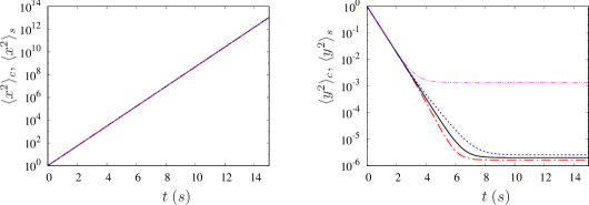
Figure 1 displays the time evolution of the lengths and for a set of parameters corresponding to those of the experiments, with and . It shows that the evolution along the dilating direction, which corresponds to an exponential growth, is almost not affected either by diffusion or diffusiophoresis. On the other hand, we observe a clear influence of diffusiophoresis on the small scale, e.g. in the contracting direction . This is especially true in the initial stage, before reaches its final value . As a consequence, the Batchelor scale is affected by diffusiophoresis so that the small scale becomes finer in the salt-attracting case () while it is coarser in the salt-repelling case (), which is consistent with experimental results obtained in Mauger et al. (2016). The Batchelor scale can be computed as , where . This relationship could serve as a definition for an effective diffusivity as was initially proposed in Deseigne et al. (2014) to interpret the salt-repelling case, although it can be seen in equation (23) that the evolution of is not obtained by replacing by in equation (13). Diffusiophoresis does not result in a process that can be considered as purely diffusive, with an effective diffusivity, as already stressed in Volk et al. (2014).
3 Dispersion in a shear flow
3.1 Shear dispersion of salt
The second problem we address is shear dispersion of Gaussian patches of salt and colloids under the action of the linear velocity field (). We define again the Péclet numbers using the () direction for both salt and colloid .
Applying the method of moments, one gets the coupled set of equations:
| (24) | |||||
| (25) | |||||
| (26) |
which can be integrated with initial conditions to obtain
| (27) | |||||
| (28) | |||||
| (29) |
Inserting those functions in expression (8), one recovers the Gaussian solution to this problem obtained by Okubo (1967). As can be observed, , and are increasing functions of time with a diffusive growth in the () direction and a super diffusive growth in the () direction, although it could have been expected that the patch is compressed in some direction. This is due to the shear motion which tilts the patch toward the () direction as indicated by the growth of . It is possible to define the variance of a large scale and of a small scale by using the principal axes of the quadratic form . With these new axes, one has , and:
| (30) | |||||
| (31) |
so that the area of the patch is . As opposed to the previous case of pure deformation, the small scale does not converge toward a final value as shown in figure (2). The small scale is first compressed as expected, but reaches a minimum value before slowly increasing again toward infinity. This is because here diffusion cannot be balanced in any direction as none of the () or () directions are dilating nor compressing as the eigenvalues of the velocity gradient matrix are zero.
3.2 Shear dispersion of colloids under diffusiophoresis
Due to the action of shear which tilts the salt patch, the diffusiophoretic drift is now more complex. However is still a linear velocity field as is Gaussian, and involves gradients in all directions:
| (32) |
Taking moments of equation (2) with this more general velocity field, moments of the colloid concentration field are solutions of a system of fully coupled ODEs:
| (33) | |||
| (34) | |||
| (35) |
with same initial conditions as in the previous case. Such system has no known analytical solutions but can be integrated numerically for any set of parameters using standard techniques (fourth-order Runge-Kutta in the present case). As already observed for the salt, the colloid patch is expected to be tilted toward () axis so that we introduce its principal axes and compute
| (36) | |||||
| (37) |
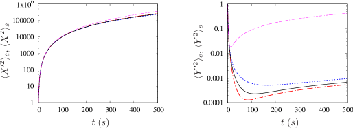
Note that the axes for the salt and colloids do not coincide so that the small and large scales are not measured exactly along the same direction. Figure 2 displays the time evolution of the lengths and for a set of parameters corresponding to those of the experiments, with and . As already observed in the case of compression, we find that diffusiophoresis mostly affects the small scale which again becomes finer in the salt-attracting case () while it is coarser in the salt-repelling case (), the effect being slightly larger in this second configuration.
4 Mixing and compressibility

4.1 Compressibility and its link to changes in colloid concentration
In the two previous cases, we found that both salt and colloid concentration profiles remain Gaussian with areas and changing as functions of time. Because the total colloid and salt content are conserved, the areas of the patches can be used as a measure of the respective concentrations and .
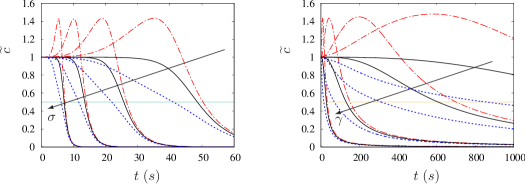
As all equations are linear, we will focus on the non-dimensional quantities and . Figure 3 displays the time evolution of the concentrations and for the two cases of pure deformation (left) and pure shear (right), with the very same set of parameters and s-1. As already observed in chaotic advection (Deseigne et al. (2014); Volk et al. (2014)), the concentration decays much faster in the salt-repelling configuration (enhanced mixing), while it first increases toward a maximum in the salt-attracting configuration, resulting in a delayed mixing. This is here a direct consequence of the patches aspect ratio evolution which is strongly modified by diffusiophoresis at short time. All these changes can be interpreted by examining the area dilation factor, , defined as:
| (38) |
This equation establishes a direct link between the evolution of and compressible effects as pointed out in Volk et al. (2014). Indeed, using second-order moments for both salt and colloids , one obtains the general expression:
| (39) | |||||
| (40) |
In the case of pure deformation, the cross-term vanishes. Using equations (19) and (21), the area dilation can be rewritten:
| (41) |
Equation (41) shows that the area of the colloid patch varies as a sum of the diffusion, which tends to make it grow in size, and diffusiophoresis: when (salt-attracting configuration), the area first contracts because here , while the patch spreads faster when (salt-repelling configuration). It is interesting to note that the diffusiophoretic contribution to the dilation factor is exactly , in agreement with the colloid concentration budget established in Volk et al. (2014), or with more general results for inertial particles (Metcalfe et al. (2012)).
In the case of shear dispersion, the cross-term does not vanish as both salt and colloid patches are tilted by the flow. Using equations (33), (34) and (35), the area dilation has the more complex form:
| (42) |
Introducing the two systems of principal axes for the colloids , and for the salt , one can obtain a similar expression as in the case of pure deformation. The equation writes:
| (43) |
from which it is visible that the second term is again exactly . This shows that the interpretation of diffusiophoresis in terms of a competition/cooperation between diffusion and compressible effects is very robust and general. In both cases we find that the flow parameters do not enter the result explicitly because is divergence free. The effect of the velocity field is in fact hidden and it is only when investigating the evolution of the various length scales that its properties are directly visible.
4.2 Evolution of the mixing time in the limit
We now investigate how much time is needed to mix the patches in the different cases. From the previous section, it may be thought that mixing processes in both flows are similar because the two graphics displayed in figure 3 look similar on first inspection. However, because of exponential stretching in the pure deformation versus algebraic stretching in the pure shear, the mixing efficiencies of these two flows are in fact very different, although they correspond to the same Péclet number . This can be quantified by the mixing time, , defined as the time when the relative concentration is divided by : . From figure 3, we have , which is one order of magnitude smaller than .
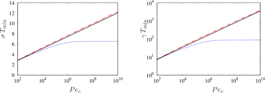
Figure 4 displays the evolution of in both cases when increasing by decreasing the colloid diffusion coefficient with all other parameters maintained fixed so that the salt Péclet number remains 222Parameters are , , , the shear rate being (deformation) and (shear).. In the case of pure deformation, increases logarithmically with , and we find that the ratio of the mixing times with and without diffusiophoresis is nearly constant at moderate Péclet number . Such a result can be explained by recalling that the large scale is weakly affected by diffusiophoresis and expands exponentially while the small scale is compressed toward the modified Batchelor scale . Defining as the time needed for the concentration to be half of its initial value, one obtains:
| (44) | |||||
| (45) |
which gives a qualitative picture of how the is affected by diffusiophoresis at moderate .
In the case of pure shear, is found to increase as a power law . Such algebraic scaling is a direct consequence of equation (29), and is typical of shear dispersion (Young et al. (1982); Rhines & Young (1983)). It is obtained by assuming that the patch grows as in the direction so that it has doubled in size in a time (here ). In this second case too, we find that in the moderate Péclet number range the mixing time is always slightly larger in the salt-attracting configuration () whereas is smaller in the salt-repelling configuration (). These observations are consistent with previous experimental and numerical studies of the mixing time (Deseigne et al. (2014); Volk et al. (2014)), especially in the case of pure deformation for which the mixing time presents the same logarithmic scaling as in the chaotic regime due to the action of compression.
In the high Péclet number range, we observe that saturates (close to and respectively). This is a very interesting behaviour because it shows that the colloids can be mixed efficiently although they have a vanishingly small diffusion coefficient. Such a property is uncommon, and is not explained by the two qualitative pictures given previously.
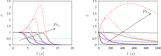
In order to understand this behaviour we plot the evolution in figure 5 for four values of the Péclet number . From figure 5, we observe that increasing the Péclet number results in a shift of toward larger times both for the reference and the salt-attracting configuration so that increases at increasing . On the opposite, no such shift is observed in the salt-repelling configuration for which increasing the Péclet number no longer changes the evolution of at short time as soon as , and it is only on a longer time scale that differences between the curves can be observed. We thus conclude that the saturation values reported above strongly depends on the precise definition of . Indeed, defining as the time needed to divide the concentration by ( decrease) would extend the range of Péclet number in which we observe an increase, with larger saturation values. If this shows that the present result is robust, it points out the difficulty of defining a mixing efficiency through a single quantity, such as , as soon as the curves change their shape when varying the parameters.
4.3 The maximum concentration does not depend on flow properties ().
When investigating the influence of the colloid diffusivity in the salt-attracting case (figure 5), it appears that reaches a maximum value which increases when decreasing . Moreover this maximum of concentration seems not to depend directly on the flow. Indeed, the maximum is found to be nearly the same in the two cases of deformation and shear displayed in figure 5 (see also figure 3). Moreover, all parameters the same except or , we observe in figure 6 that is insensitive to the stirring properties of the flow. In this large Péclet number range , seems to depend only on chemical properties and initial lengths.
A qualitative analysis developed below shows that in the case of initially round patches, the maximum of colloid concentration is well predicted by the relation:
| (46) |
In order to establish this relation, we first start with equations (39) and (43) which describe the evolution of both salt and colloids compressibilities, and rewrite them as:
| (47) | |||||
| (48) |
where we used the principal axes of both Gaussian distributions. In the initial stage of colloid mixing, diffusive effects are negligible as compared to diffusiophoretic effect because , so that
| (49) |
In this first stage, the area of both species are related to each other by the relation
| (50) |
which explains why all curves for the salt-attracting configuration follow the same initial evolution in figure 5 where only is varied. We will assume that this relation holds for such that , which is an approximation as the role of is neglected and may lead to a slight overestimation of . When reaches its maximum value, diffusive and diffusiophoretic effects compensate so that reaches a minimum and its time derivative is zero. As the small scales of both species are much smaller than the corresponding large scales, and are then linked by the relation (equation (48)):
| (51) |
In the case of initially round patches, the large scales of both species are only weakly affected by diffusion and diffusiophoresis so that at any time. This leads to the relation:
| (52) |
which we chose to write
| (53) |
This last relation can be combined with equation (50) to get the formula given in equation (46). Note that in the case of pure deformation and directions decouple so that equation (46) holds also for non-round patches (i.e. with arbitrary initial aspect ratios). Note also that we used the hypothesis that the distributions of salt and colloids possess a large and a small scale, so that equation (46) would not hold in the absence of flow (pure diffusiophoresis).
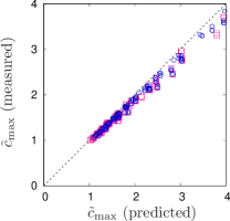
The prediction of has been tested with initially round patches in both cases of pure shear and deformation by varying independently all parameters (, , , , ) over two decades with fixed values s-1 and s-1. Figure 7 displays the maximum concentration measured from as a function of the predicted value. It is remarkable that the maximum is very well predicted by the relation (46) with less than error. This shows that the hypothesis of taking into account colloid diffusion only very close to the maximum is a good approximation. As seen from this figure is an other striking result: by setting the experimental configuration of a small salt patch ( mm) and a larger colloid patch ( mm), it is in principle possible to increase the colloid concentration by a factor larger than , which would correspond to strong demixing of the colloids.
5 Conclusion
We have studied analytically the dispersion of patches of salt and colloids in linear velocity fields. The velocity fields (pure deformation and pure shear) were chosen to correspond to fundamental examples at the heart of our understanding of mixing (Bakunin (2011)). Assuming the patches were initially released with Gaussian profiles, both cases could be analytically solved almost entirely so that results could be obtained for any set of parameters.
An analytical solution was obtained in the case of pure deformation, which showed that diffusiophoresis led to a modification of the Batchelor scale . The case of pure shear was found to be more complex, but equations for the evolutions of colloid concentration moments were obtained and solved numerically for various sets of parameters.
Using the area of the patches , the evolution of the colloid global concentration (rescaled by its initial value) was studied. A prediction for the time, , needed to decrease the concentration by a factor 2 was obtained. In both cases, we found that in the moderate Péclet number range the mixing time is always slightly larger in the salt-attracting configuration () whereas is smaller in the salt-repelling configuration (). These observations are consistent with previous experimental and numerical studies of the mixing time (Deseigne et al. (2014); Volk et al. (2014)), especially in the case of pure deformation for which the mixing time presents the same logarithmic scaling as in the chaotic regime due to the action of compression.
In all cases, the evolution of the concentration was intriguingly similar to the one observed experimentally in chaotic mixing, presenting a maximum in the salt-attracting configuration as the colloid concentration is first amplified before being attenuated.
Using arguments based on compressibility, it was possible to obtain a prediction of the maximum concentration when dealing with initially round patches.
This prediction involves the existence of a flow, but does not involve the flow parameters, and compares very well with numerical and analytical results.
Finally, we stress that while established in the case of linear flows, it also gives the correct order of magnitude (less than error) in the case of diffusiophoresis with chaotic advection in our numerical paper (Volk et al. (2014)).
This points out that diffusiophoretic effects are not changed when increasing stirring. This observation also holds for the mixing time as we found that the ratio does not depend on the shear rate.
Acknowledgments This collaborative work was supported by the French research programs ANR-16-CE30-0028 and LABEX iMUST (ANR-10-LABX-0064) of Université de Lyon, within the program“Investissements d’Avenir” (ANR-11-IDEX-0007) operated by the French National Research Agency (ANR).
References
- Abécassis et al. (2009) Abécassis, B., Cottin-Bizonne, C., Ybert, C., Ajdari, A. & Bocquet, L. 2009 Osmotic manipulation of particles for microfluidic applications. New Journal of Physics 11 (7), 075022.
- Anderson (1989) Anderson, J. L. 1989 Colloid transport by interfacial forces. Annu. Rev. Fluid. Mech. 21, 61–99.
- Aris (1956) Aris, R. 1956 On the dispersion of a solute in a fluid flowing through a tube. Proceedings of the Royal Society of London A: Mathematical, Physical and Engineering Sciences 235 (1200), 67–77.
- Bakunin (2011) Bakunin, Oleg G., ed. 2011 Chaotic Flows. Springer.
- Banerjee et al. (2016) Banerjee, Anirudha, Williams, Ian, Azevedo, Rodrigo Nery, Helgeson, Matthew E. & Squires, Todd M. 2016 Soluto-inertial phenomena: Designing long-range, long-lasting, surface-specific interactions in suspensions. Proceedings of the National Academy of Sciences 113 (31), 8612–8617.
- Batchelor (1959) Batchelor, G. K. 1959 Small-scale variation of convected quantities like temperature in turbulent fluid part 1. general discussion and the case of small conductivity. Journal of Fluid Mechanics 5 (1), 113–133.
- Birch et al. (2008) Birch, D.A., Young, W.R. & Franks, P.J.S. 2008 Thin layers of plankton: Formation by shear and death by diffusion. Deep Sea Research Part I: Oceanographic Research Papers 55 (3), 277 – 295.
- Deseigne et al. (2014) Deseigne, J., Cottin-Bizonne, C., Stroock, A. D., Bocquet, L. & Ybert, C. 2014 How a ”pinch of salt” can tune chaotic mixing of colloidal suspensions. Soft Matter 10, 4795–4799.
- Mauger et al. (2016) Mauger, Cyril, Volk, Romain, Machicoane, Nathanaël, Bourgoin, Michaël, Cottin-Bizonne, Cécile, Ybert, Christophe & Raynal, Florence 2016 Diffusiophoresis at the macroscale. Phys. Rev. Fluids 1, 034001.
- Metcalfe et al. (2012) Metcalfe, Guy, Speetjens, MFM, Lester, DR & Clercx, HJH 2012 Beyond passive: chaotic transport in stirred fluids. In Advances in Applied Mechanics, , vol. 45, pp. 109–188. Elsevier.
- Okubo (1967) Okubo, A . 1967 The effect of shear in an oscillatory current on horizontal diffusion from an instantaneous source. int. J. Oceanol. Limnol 1, 194–204.
- Rhines & Young (1983) Rhines, P. B. & Young, W. R. 1983 How rapidly is a passive scalar mixed within closed streamlines? Journal of Fluid Mechanics 133, 133–145.
- Taylor (1953) Taylor, G. I. 1953 Dispersion of soluble matter in solvent flowing slowly through a tube. Proceedings of the Royal Society of London A: Mathematical, Physical and Engineering Sciences 219 (1137), 186–203, arXiv: http://rspa.royalsocietypublishing.org/content/219/1137/186.full.pdf.
- Townsend (1951) Townsend, A. A. 1951 The diffusion of heat spots in isotropic turbulence. Proceedings of the Royal Society of London A: Mathematical, Physical and Engineering Sciences 209 (1098), 418–430.
- Volk et al. (2014) Volk, R., Mauger, C., Bourgoin, M., Cottin-Bizonne, C., Ybert, C. & Raynal, F. 2014 Chaotic mixing in effective compressible flows. Phys. Rev. E 90, 013027.
- Young et al. (1982) Young, W. R., Rhines, P. B. & Garrett, C. J. R. 1982 Shear-flow dispersion, internal waves and horizontal mixing in the ocean. Journal of Physical Oceanography 12 (6), 515–527.