Diffusion Enhancement of Brownian Motors Revealed by a Solvable Model

Abstract

A solvable model is proposed and analyzed to reveal the mechanism underlying the diffusion enhancement recently reported for a model of molecular motors and predicted to be observed in the biological rotary motor $\rm F_{1}$-ATPase. It turns out that the diffusion enhancement for the present model can approximately described by a random walk in which the waiting time for a step to occur is exponentially distributed and it takes nonzero time to proceed forward by the step. It is shown that the diffusion coefficient of such a random walk can significantly be increased when the average waiting time is comparable to the average stepping time.

I Introduction

There can be various ways to produce an effective diffusion coefficient larger than what is expected from the Einstein relation. A classical example of such diffusion enhancement is the swimming of bacteria Berg (1993). A bacterium swims with a constant speed and occasionally changes its swimming direction. The resulting motion is a random walk with an effective diffusion coefficient much larger than that of the Brownian motion it would undergo if it stopped swimming. This diffusive motion helps bacteria find their foods or move away from harmful environments, for example. Recently, it was found that a Brownian particle moving in a one-dimensional periodic potential exhibits the diffusion enhancement under a constant external force of magnitude close to the maximum slope of the potential Costantini and Marchesoni (1999); Reimann et al. (2001, 2002). This phenomenon was observed experimentally in a colloidal system Speer et al. (2012), a biomolecule having a rotating subunit Hayashi et al. (2015), and DNA diffusing in an array of entropic barriers Kim et al. (2017). The diffusion enhancement also occurs in on-off ratchets Germs et al. (2013) in which an asymmetric, periodic potential for colloidal particles is switched on and off periodically, if the duration of potential-off interval is such that the root-mean square displacement of the particle by free diffusion in this interval is comparable to the periodicity of the potential.

In our previous work Shinagawa and Sasaki (2016), it is demonstrated theoretically that the diffusion enhancement can occur in molecular motors that move autonomously by consuming free energy available from the chemical reaction catalyzed by themselves if a constant external force of appropriate magnitude is applied. In particular, it is suggested that the diffusion enhancement can be observed in the F₁-ATPase, a biological rotary motor, which catalyzes the hydrolysis of adenosine triphosphate (ATP). It has turned out that the mechanism of enhancement in the case of high ATP concentration is essentially the same as the one for the particle in a tilted periodic potential Costantini and Marchesoni (1999); Reimann et al. (2001, 2002). On the other hand, the mechanism in the case of low ATP concentration has not been clarified yet. The purpose of the present work is to study the diffusion of a simplified model of molecular motors to elucidate the mechanism of diffusion enhancement characteristic of chemically driven systems. In what follows effective diffusions coefficient will simply be called diffusion coefficients.

The models considered here and in the previous work Shinagawa and Sasaki (2016) are of ratchet type Jülicher et al. (1997); Reimann (2002); Kawaguchi et al. (2014), in which a moving part of the motor (e.g., the rotor in a rotary motor) is represented by a Brownian particle subject to a potential, which is switched to another upon a chemical transition associated with the reaction catalyzed by the motor. In the model used in the previous paper Shinagawa and Sasaki (2016), an external force, as well as rate constants, can control the transition rates because the transition rates are assumed to depend on the particle position, which is affected by the force; the dependence of the diffusion coefficient on the force for given rate constants exhibits enhancement in a certain range of the force. By contrast, an external force is not included in the model of the present paper, and a rate constant is varied to study the diffusion enhancement. Another simplification is that chemical transitions are supposed to take place only when the particle is located at particular points, which enable us to obtain a closed-form expression for the diffusion coefficient.

The paper is organized as follows. The model is introduced in the next section, and the closed-form expressions for the velocity and diffusion coefficient are given in Sec. III. Explicit calculations of the diffusion coefficient are carried out for a model with piecewise linear potentials in Sec. IV, where the diffusion enhancement is demonstrated. In Sec. V, we discuss the mechanism of the diffusion enhancement observed in Sec. IV on the basis of a simple random walk, which we call an extended Poisson walk. Concluding remarks will be given in Sec. VI. Some of the details of calculations and expressions are given in Appendices.

II Potential-switching ratchet

We consider a variant of pulsating ratchets as a model of biological molecular motor Jülicher et al. (1997); Reimann (2002); Kawaguchi et al. (2014). The motor is modeled as a Brownian particle moving in one dimension, along the $x$ axis, subject to potentials $V_{n}(x)$ ($n=0,\pm 1,\pm 2,\dots$) of identical shapes arranged periodically with period $l$ as shown in Fig. 1(a), i.e., they satisfy

$$V_{n+1}(x)=V_{n}(x-l)\quad(n=0,\pm 1,\pm 2,\dots).$$ (1)

The potentials are assumed to be unbounded above. Only one of the potentials acts on the particle at a time, say $V_{n}$, and it is stochastically switched to $V_{n+1}$ or $V_{n-1}$. The motor will be said to be in state $n$ if potential $V_{n}$ is acting. The dynamics of the particle is assumed to be over-damped. The diffusion coefficient of the particle in the absence of the potentials is given by the Einstein relation $D_{0}=k_{\text{B}}T/\gamma$, where $\gamma$ is the coefficient of the drag force on the particle from the surrounding fluid, $T$ is the temperature, and $k_{\text{B}}$ is the Boltzmann constant.

Let $P_{n}(x,t)\,dx$ be the probability to find the motor in state $n$ and the particle in the interval $(x,x+dx)$ on the $x$ axis at time $t$, and $w_{n}^{\pm}(x)$ be the rate of transition from state $n$ to state $n\pm 1$ when the particle is located at $x$. Then the time evolution of $P_{n}(x,t)$ is described by the Fokker-Planck equations,

$$\frac{\partial P_{n}}{\partial t}+\frac{\partial J_{n}}{\partial x} =-(w_{n}^{+}+w_{n}^{-})P_{n}$$

$$\quad{}+w_{n-1}^{+}P_{n-1}+w_{n+1}^{-}P_{n+1},$$ (2)

where $J_{n}$ is the probability current in state $n$ defined by

$$J_{n}\equiv-D_{0}\left(\frac{\partial}{\partial x}+\frac{dU_{n}}{dx}\right)P_{n}$$ (3)

with

$$U_{n}(x)\equiv V_{n}(x)/k_{\text{B}}T$$ (4)

being the dimensionless potential. We remark that the arguments given in this section applies also to the case in which a constant external force $F$ is applied to the particle if the right-hand side of Eq. (4) is replaced by $[V_{n}(x)-Fx]/k_{\text{B}}T$.

We assume that the transition from one state to another takes place when the particle is located at a particular position (this corresponds to the idea that the change in chemical state of a motor protein occurs when it is in a particular conformation Jülicher et al. (1997)), and adopt the following expressions for $w_{n}^{\pm}(x)$:

$$w_{n}^{\pm}(x)=\omega_{\pm}\delta(x-a_{\pm}-nl),$$ (5)

where $\delta(x)$ is the delta function, $\omega_{\pm}$ are positive constants, and $a_{+}$ and $a_{-}$ are constants satisfying $a_{-}=a_{+}-l$; see Fig. 1(a). The transition $n\to n+1$ and its reversal occur at $x=a_{+}+nl=a_{-}+(n+1)l$. Supposing that the “forward” transition $n\to n+1$ is triggered by a chemical reaction by which the free energy of the environment is decreased by $\Delta\mu$, we have the relation

$$\omega_{+}/\omega_{-}=\exp\left[U_{0}(a_{+})-U_{0}(a_{-})+\Delta\mu/k_{\text{B}}T\right]$$ (6)

from the condition of local detailed balance.

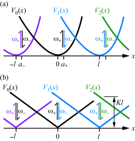
Figure 1: (Color online) Generic (a) and specific (b) models of molecular motors considered in this work. The motor is represented by a Brownian particle subject to one of the potentials $V_{n}(x)$ at a time. The potential is switched from $V_{n}$ to $V_{n+1}$ or $V_{n-1}$ stochastically with rates proportional to $\omega_{+}$ and $\omega_{-}$, respectively, if the particle is located at $x=a_{+}+nl$ or $a_{-}+nl$; we set $a_{+}=0$ and $a_{-}=-l$ for (b).

The velocity $v$ and the diffusion coefficient $D$ of the motor are defined by

$$v\equiv\lim_{t\to\infty}\frac{\langle x(t)-x(0)\rangle}{t},D\equiv\lim_{t\to\infty}\frac{\langle[x(t)-x(0)-vt]^{2}\rangle}{2t},\quad$$ (7)

where $x(t)$ is the location of the particle (motor) at time $t$ and the angular brackets indicate the statistical average. The velocity can be obtained from the steady-state solutions $P_{n}(x)$ of the Fokker-Planck equations (II), which satisfy the “periodicity condition” $P_{n}(x)=P_{0}(x-nl)$. Let $P(x)$ be the rescaled $P_{0}(x)$ so that it satisfies

$$\int_{-\infty}^{\infty}P(x)\,dx=1.$$ (8)

Then we have Jülicher et al. (1997); Reimann (2002)

$$v=\int_{-\infty}^{\infty}f(x)P(x)\,dx,\quad f(x)\equiv-D_{0}\,dU_{0}(x)/dx.$$ (9)

To calculate the diffusion coefficient, we need to obtain the auxiliary function $Q(x)$ that satisfies

$$\frac{d}{dx}\left[D_{0}\frac{d}{dx}-f(x)\right]Q(x)-\left[w_{0}^{+}(x)+w_{0}^{-}(x)\right]Q(x)$$

$$\qquad{}+w_{0}^{+}(x+l)Q(x+l)+w_{0}^{-}(x-l)Q(x-l)$$

$$\quad{}=\left[v-f(x)+2D_{0}\frac{d}{dx}\right]P(x)$$ (10)

and the boundary condition that $Q(x)\to 0$ as $|x|\to\infty$. The diffusion coefficient is calculated as Harms and Lipowsky (1997); Sasaki (2004); Shinagawa and Sasaki (2016)

$$D=D_{0}+\int_{-\infty}^{\infty}\left[f(x)-v\right]Q(x)\,dx.$$ (11)

III Closed-Form Expressions

The specific functional forms of $w_{n}^{\pm}(x)$ given in Eq. (5) enable us to derive closed form expressions for $v$ and $D$, as explained in Appendix A. To express the result for $v$ concisely, we introduce constants $\zeta$, $\phi_{0}$, $\phi_{1}$, and $u_{\pm}$ defined by

$$\zeta\equiv\int_{-\infty}^{\infty}e^{-U(x)}\,dx,\quad$$ (12)

$$\phi_{0}\equiv\int_{a_{-}}^{a_{+}}e^{U(x)}\,dx,$$ (13)

$$\phi_{1}\equiv\int_{a_{-}}^{a_{+}}e^{U(y)}\,dy\int_{-\infty}^{y}e^{-U(x)}\,dx,$$ (14)

$$u_{\pm}\equiv\omega_{\pm}\exp\left[-U(a_{\pm})\right],$$ (15)

where

$$U(x)\equiv U_{0}(x).$$ (16)

Then, the velocity is expressed as

$$v=\frac{(u_{+}-u_{-})D_{0}l}{\zeta(D_{0}+\phi_{0}u_{-})+\phi_{1}(u_{+}-u_{-})}.$$ (17)

Note that we have $u_{+}>u_{-}$ for $\Delta\mu>0$ according to the detailed-balance condition (6) and that the denominator in Eq. (17) is positive since $\zeta\phi_{0}-\phi_{1}>0$, which can be verified from Eqs. (12)–(14). Therefore, Eq. (17) indicates that $v>0$ for $\Delta\mu>0$, as expected.

The result for $D$ can be expressed as

$$D=\lambda l+v\int_{-\infty}^{\infty}W(x)\,dx$$ (18)

with the constant $\lambda$ and function $W(x)$ given below. The function $W(x)$ is defined by

$$W(x)\equiv h(x)-\int_{-\infty}^{x}P(y)\,dy,$$ (19)

where the function $h(x)$ is defined by

$$h(x)\equiv\begin{cases}0&(x<a_{-}),\\ (x-a_{-})/l&(a_{-}\leq x\leq a_{+}),\\ 1&(x>a_{+}),\end{cases}$$ (20)

and the rescaled steady-state distribution $P(x)$ is given by

$$P(x)=g(x)\exp[-U(x)]$$ (21)

with

$$g(x)=\begin{cases}C_{-}&(x<a_{-}),\\ \displaystyle C_{-}-\frac{v}{D_{0}l}\int_{a_{-}}^{x}e^{U(y)}\,dy&(a_{-}\leq x\leq a_{+}),\\ C_{+}&(x>a_{+}).\end{cases}$$ (22)

Here, the constants $C_{\pm}$ are defined by

$$C_{\pm}\equiv\frac{(1+\phi_{0}u_{\mp}/D_{0})v}{(u_{+}-u_{-})l}.$$ (23)

The constant $\lambda$ in Eq. (18) is given by

$$\lambda\equiv-\frac{\zeta\psi_{0}u_{-}+\psi_{1}(u_{+}-u_{-})}{\zeta(D_{0}+\phi_{0}u_{-})+\phi_{1}(u_{+}-u_{-})},$$ (24)

where $\psi_{0}$ and $\psi_{1}$ are integrals

$$\psi_{0} \equiv\int_{a_{-}}^{a_{+}}R(x)e^{U(x)}\,dx,$$ (25)

$$\psi_{1} \equiv\int_{-\infty}^{\infty}e^{-U(x)}\,dx\int_{x}^{a_{+}}R(y)e^{U(y)}\,dy,$$ (26)

involving a new function $R(x)$ defined by

$$R(x)\equiv vW(x)-D_{0}P(x).$$ (27)

IV Model with piecewise-linear potentials

As a specific example, we consider a model with piecewise linear potentials for which $V_{0}(x)$ is given by

$$V_{0}(x)=K\left|x\right|$$ (28)

with a positive parameter $K$; see Fig. 1(b). The parameter for the locations of transitions is set as $a_{+}=0$ (which implies $a_{-}=-l$). For this model the integrals needed to calculate the velocity and diffusion coefficient can be carried out analytically, as explained below.

IV.1 Results

It is straightforward to obtain the constants involved in Eq. (17) for $v$; the results are as follows:

$$\zeta=2/\kappa,\quad\phi_{0}=\left(e^{\kappa l}-1\right)/\kappa,\quad\phi_{1}=l/\kappa,$$ (29)

$$u_{+}=\omega_{+},\quad u_{-}=\omega_{-}e^{-\kappa l},$$ (30)

where

$$\kappa\equiv K/k_{\text{B}}T.$$ (31)

Substituting expressions in Eqs. (29) and (30) into Eq. (17), we obtain the average velocity $v$ of the motor for this model:

$$v=\frac{\kappa D_{0}\left(\omega_{+}-\omega_{-}e^{-\kappa l}\right)}{\omega_{+}+(2/\kappa l)(\omega_{-}+\kappa D_{0})-(1+2/\kappa l)\omega_{-}e^{-\kappa l}}.$$ (32)

Note that $v$ monotonically increases with $\omega_{+}$, which is proportional to the forward transition rate $w_{n}^{+}(x)$, Eq. (5), and tends to the limiting value $\kappa D_{0}=K/\gamma$. This is identical to the average velocity of a particle subject to a constant external force $K$. This is because, in the limit of large $\omega_{+}$, the particle stays only on the left-side slopes of potentials $V_{n}$ of Fig. 1(b), since the potential is switched from $V_{n}$ to $V_{n+1}$ right after the particle on the left-side slope of $V_{n}$ reaches the potential minimum at $x=nl$, and this switching brings the particle to the left-side slope of $V_{n+1}$, and so on.

The expressions for the steady-state probability density $P(x)$ and the auxiliary function $W(x)$, both needed for calculating the diffusion coefficient, are presented in Appendix B. From the expressions for $W(x)$ given in Eqs. (77) and (78), we have

$$\int_{-\infty}^{\infty}W(x)\,dx=\frac{l}{2}-\frac{vl}{2\kappa D_{0}}\left(1+\frac{2}{\kappa l}\right),$$ (33)

which contributes to the second term in Eq. (18) for $D$. The integrals $\psi_{0}$ and $\psi_{1}$ defined by Eqs. (25) and (26), respectively, can be carried out by substituting Eq. (27) with $W(x)$ and $P(x)$ given in Eqs. (75)–(78) into these definitions to obtain

$$\psi_{0} =\frac{2v^{2}}{\kappa^{2}D_{0}}\left(1+\frac{\kappa l}{4}-\frac{e^{\kappa l}-1}{\kappa l}\right)-\frac{D_{0}\kappa l}{2},$$ (34)

$$\psi_{1} =\frac{vl}{2\kappa}\left(1-\frac{4}{\kappa l}\right)-\frac{v^{2}l}{2\kappa^{2}D_{0}}.$$ (35)

From these results and Eqs. (29) and (30), we find $\lambda$ defined by Eq. (24), which contributes to the first term in Eq. (18). Substituting this result for $\lambda$ together with Eq. (33) into Eq. (18) provides us with the analytic expression for $D$.

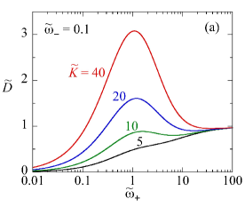
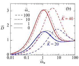
Figure 2: (Color online) Dependence of the diffusion coefficient $\tilde{D}$ on the forward transition rate $\tilde{\omega}_{+}$. (a) The results for several choices of $\tilde{K}$ are shown in the case of $\tilde{\omega}_{-}=0.1$. (b) The results for several choices of the rate $\tilde{\omega}_{-}$ of backward transition, in the cases of $\tilde{K}=40$ and 20.

The dependence of the diffusion coefficient on $\omega_{+}$ is shown in Fig. 2(a) for several choices of $K$ and a fixed value of $\omega_{-}$. The result is represented in terms of dimensionless parameters defined by

$$\tilde{D}\equiv D/D_{0},\quad\tilde{\omega}_{\pm}\equiv l\omega_{\pm}/D_{0},\quad\tilde{K}\equiv lK/k_{\text{B}}T.$$ (36)

We observe that $\tilde{D}$ increases monotonically with $\tilde{\omega}_{+}$ for $\tilde{K}=5$, whereas it has a peak around at $\tilde{\omega}_{+}\sim 1$ for large values of $\tilde{K}$. The peak height increases with $\tilde{K}$. In either case, $\tilde{D}$ tents to 1 ($D$ tends to $D_{0}$) from below as $\tilde{\omega}_{+}\to\infty$ (therefore, the curve $\tilde{D}(\tilde{\omega}_{+})$ exhibits a shallow dip when it has a peak). The reason why $D$ converges to $D_{0}$ is that, in this limiting case, the particle always experiences a constant external force as explained above, and hence its diffusion coefficient is the same as that of a free particle. The increase in the diffusion coefficient controlled by the transition rate shown in Fig. 2(a) is the diffusion enhancement in our model for molecular motors.

Figure 2(b) shows how the diffusion enhancement is affected by the rate parameter $\tilde{\omega}_{-}$ of the backward transition for the cases of $\tilde{K}=20$ and 40. In the both cases, the peak height does not depend very much on $\tilde{\omega}_{-}$, while the peak position moves to the right (the direction of increasing $\tilde{\omega}_{+}$) as $\tilde{\omega}_{-}$ increases.

IV.2 Limit of small $\omega_{-}$

We see from Fig. 2(b) that, as $\tilde{\omega}_{-}$ decreases, $\tilde{D}$ as a function of $\tilde{\omega}_{+}$ for a given $\tilde{K}$ converges to a certain function [indicated by the solid line in Fig. 2(b)]. This limiting function is obtained by setting $\omega_{-}=0$ in the expression for $D$ obtained above; we have

$$D=\frac{v^{3}}{\kappa^{3}D_{0}^{2}}\left[1+\frac{2D_{0}}{l\omega_{+}}+2\kappa l\left(\frac{D_{0}}{l\omega_{+}}\right)^{2}\right]$$ (37)

with the limiting velocity

$$v=\frac{\kappa D_{0}\omega_{+}}{\omega_{+}+2D_{0}/l},$$ (38)

which has the “Michaelis–Menten type” dependence Howard (2001) on $\omega_{+}$. We are interested in this limiting case, because the backward transition rate is negligibly small under the condition for the diffusion enhancement to be observed in the previous work Shinagawa and Sasaki (2016) for low ATP concentrations; the mechanism of the enhancement in this situation has not been clarified, as mentioned in the introduction.

Equation (37) tells that if $\tilde{K}>4+2\sqrt{3}\approx 7.46$ then function $\tilde{D}(\tilde{\omega}_{+})$ has a peak at

$$\tilde{\omega}_{+}^{\text{max}}=\tilde{K}/2-\sqrt{\tilde{K}^{2}/4-2\tilde{K}+1}$$ (39)

and a local minimum at $\tilde{\omega}_{+}^{\text{min}}$ give by Eq. (39) with the sign of the last term being changed. The dependence of $\tilde{\omega}_{+}^{\text{max}}$ and $\tilde{\omega}_{+}^{\text{min}}$ on $\tilde{K}$ are shown in Fig. 3(a); and the peak height $\tilde{D}_{\text{max}}$ and the value of $\tilde{D}$ at the local minimum $\tilde{D}_{\text{min}}$ are plotted against $\tilde{K}$ in Fig. 3(b). It is seen that the peak position $\tilde{\omega}_{+}^{\text{max}}$ tends to unity as

$$\tilde{\omega}_{+}^{\text{max}}\approx 1+3/\tilde{K}$$ (40)

in the large $\tilde{K}$ limit, whereas the peak height $\tilde{D}_{\text{max}}$ increases almost linearly in $\tilde{K}$. In fact, we have

$$\tilde{D}_{\text{max}}\approx 2\tilde{K}/27+1/9$$ (41)

for large $\tilde{K}$. Diffusion coefficient of more than twice that of free diffusion ($\tilde{D}>2$) can be achieved for $\tilde{K}\gtrsim 25$. The mechanism of the diffusion enhancement in this limiting case is discussed in the next section.

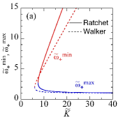
Figure 3: (Color online) Dependence of (a) $\tilde{\omega}_{+}^{\text{max}}$ and $\tilde{\omega}_{+}^{\text{min}}$ and (b) $\tilde{D}_{\text{max}}$ and $\tilde{D}_{\text{min}}$ on $\tilde{K}$. Here, $\tilde{\omega}_{+}^{\text{max}}$ and $\tilde{\omega}_{+}^{\text{min}}$ are the positions of the peak and the local minimum of function $\tilde{D}(\tilde{\omega}_{+})$, respectively, and $\tilde{D}_{\text{max}}$ and $\tilde{D}_{\text{min}}$ are the values of $\tilde{D}$ at these locations. The solid lines are the results for the ratchet model given in Eq. (37) in the limit of $\tilde{\omega}_{-}=0$, and the dashed lines are those of the extended Poisson walk, Eq. (45).

V Extended Poisson walk

V.1 Diffusion of a random walker

For qualitative understanding of the diffusion enhancement we have observed in the preceding section, let us take a look at the motion of the particle for the case in which the backward transition can be neglected (Section IV B). The particle moves on the left-side slope of one of the V-shaped potentials shown in Fig. 1 toward its bottom point right after a forward transition occurs. After reaching the bottom, it moves around the potential minimum until another forward transition occurs. Suppose that we plot the particle positions $x$ agains time $t$ at the occasions a forward transition occurs and the particle reaches the bottom of a potential for the first time. If we connect these points with line segments, we will have a trajectory like the one shown in Fig. 4.

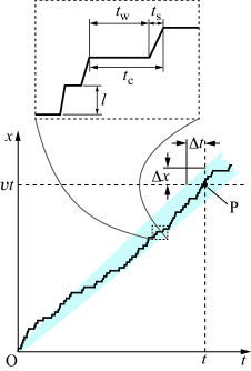
Figure 4: (Color online) Trajectory of a random walker on a one-dimensional lattice of lattice constant $l$, which mimics the trajectory of the particle in the ratchet model. It stays on a lattice site waiting to step forward for a period of time $t_{\text{w}}$, and it takes nonzero time $t_{\text{s}}$ to make a forward step.

Such a trajectory may be viewed as a trajectory of a random walker on a one-dimensional lattice of lattice spacing $l$. The walker stays on a lattice site until it takes a forward step. The time $t_{\text{w}}$ for the walker to wait at the site (see the upper part of Fig. 4) is a random variable. It also takes a nonzero time $t_{\text{s}}$ for the walker to move to the next lattice site; the stepping time $t_{\text{s}}$ is also a random variable. Let $t_{\text{c}}$ be the period of a cycle from the start of a waiting to the end of the stepping that follows it (Fig. 4), i.e., $t_{\text{c}}=t_{\text{w}}+t_{\text{s}}$. The walker moves forward by distance $l$ every time it completes a cycle. Hence, the average velocity $v$ of the walker can be expressed as

$$v=l/\tau_{\text{c}}$$ (42)

in terms of the average $\tau_{\text{c}}$ of $t_{\text{c}}$.

The diffusion coefficient of the walker may be obtained as follows. Consider a collection of trajectories of the walker starting from $x=0$ at $t=0$. The shaded area in Fig. 4 represents the region traversed by a large fraction of the trajectories. Let P the point on the line $x=vt$ that runs through the center of this region. Denoting the half-width of this region measured along the vertical line passing through this point by $\Delta x$ (see Fig. 4), the diffusion coefficient can be estimated as

$$D=\Delta x^{2}/2t=(v\Delta t)^{2}/2t,$$ (43)

where $t$ is the abscissa of point P and $\Delta t$ is the half-width of the shaded region in Fig. 4 measured along the horizontal line passing through point P. Now, $\Delta t$ can be calculated from the variance $\sigma_{\text{c}}^{2}$ of the cycle time $t_{\text{c}}$ of the walker as follows. The walker completes $N=vt/l$ cycles while it travels distance $vt$, which is the ordinate of point P. The variance of the time needed to complete $N$ cycles is $N\sigma_{\text{c}}^{2}$, and this variance is identified as $\Delta t^{2}$. Hence we have

$$\Delta t^{2}=N\sigma_{\text{c}}^{2}=vt\sigma_{\text{c}}^{2}/l.$$ (44)

Substitution of this expression and Eq. (42) into Eq. (43) results in

$$D=\sigma_{\text{c}}^{2}l^{2}/2\tau_{\text{c}}^{3}.$$ (45)

It should be noted that this expression for $D$ obtained by the qualitative arguments agrees exactly with the one derived by mathematically rigorous calculations Svoboda et al. (1994); Schnitzer and Block (1995); see also Reimann et al. (2001, 2002).

Let us assume that the waiting of the walker is a Poisson process and hence the waiting time $t_{\text{w}}$ is distributed exponentially as

$$f(t_{\text{w}})=k\exp(-kt_{\text{w}})$$ (46)

with a rate constant $k$, which is supposed to be related with the forward transition rate of our model of molecular motor. Then the average $\tau$ and the variance $\sigma^{2}$ of $t_{\text{w}}$ are given by $\tau=1/k$ and $\sigma^{2}=1/k^{2}=\tau^{2}$, respectively. If the stepping time $t_{\text{s}}$ is zero, the walker undergoes a Poisson random walk van Kampen (2007). A walk with nonzero $t_{\text{s}}$ may be called an extended Poisson walk. The average and variance of the stepping time $t_{\text{s}}$ will be denoted by $\tau_{\text{s}}$ and $\sigma_{\text{s}}^{2}$, respectively. Since the waiting and stepping are statistically independent, the average of $t_{\text{c}}=t_{\text{w}}+t_{\text{s}}$ are given as the sum of the averages of $t_{\text{w}}$ and $t_{\text{s}}$: $\tau_{\text{c}}=\tau+\tau_{\text{s}}$. Similarly, we have $\sigma_{\text{c}}^{2}=\tau^{2}+\sigma_{\text{s}}^{2}$. Hence, the expressions in Eqs. (42) and (45) are rewritten as

$$v=\frac{l}{\tau+\tau_{\text{s}}},\quad D=\frac{l^{2}(\tau^{2}+\sigma_{\text{s}}^{2})}{2(\tau+\tau_{\text{s}})^{3}}.$$ (47)

Now, we examine the dependence of $D$ given in Eq. (47) on the average waiting time $\tau$. If the waiting time is vanishingly small, the diffusion coefficient is determined by the stepping process, which yields

$$D_{\text{s}}=\sigma_{\text{s}}^{2}l^{2}/2\tau_{\text{s}}^{3}.$$ (48)

As $\tau$ increases from zero, both the denominator and the numerator in the expression for $D$ in Eq. (47) increase. It is easy to see that the increase in the denominator exceeds that in the numerator if $\tau$ is small enough or large enough, implying that $D$ decreases with increasing $\tau$ in these regions. On the other hand, if $\sigma_{\text{s}}$ is much smaller than $\tau_{\text{s}}$, then there is a region of $\tau$ where inequalities $\sigma_{\text{s}}\ll\tau\ll\tau_{\text{s}}$ hold. In this situation, we have significantly enhanced diffusion coefficient $D\sim D_{\text{s}}(\tau/\sigma_{\text{s}})^{2}$ compared with $D_{\text{s}}$.

Precise calculations show that there is a region of $\tau$ where $D$ given in Eq. (47) increases with $\tau$ if $\sigma_{\text{s}}/\tau_{\text{s}}<1/\sqrt{3}\approx 0.577$, which indicates that function $D(\tau)$ has a peak, since $D$ decreases for large $\tau$ as explained above. The height of this peak exceeds $D_{\text{s}}$ (indicating diffusion enhancement) if $\sigma_{\text{s}}/\tau_{\text{s}}<\left(2/\sqrt{3}-1\right)^{1/2}\approx 0.393$. These results are demonstrated in Fig. 5, where the dimensionless diffusion coefficient $D/D_{\text{s}}$ is plotted against the dimensionless waiting time $\tau/\tau_{\text{s}}$ for several choices of $\sigma_{\text{s}}/\tau_{\text{s}}$. As expected from the qualitative argument given in the preceding paragraph, we see that the diffusion coefficient is significantly enhanced for small enough $\sigma_{\text{s}}/\tau_{\text{s}}$ (see the graph of $\sigma_{\text{s}}/\tau_{\text{s}}=0.2$). In the limit of small $\sigma_{\text{s}}/\tau_{\text{s}}$, the location $\tau_{\text{max}}$ and the height $D_{\text{max}}$ of the peak in $D(\tau)$ due to the diffusion enhancement can be estimated to be

$$\tau_{\text{max}}\approx 2\tau_{\text{s}},\quad D_{\text{max}}\approx 2l^{2}/27\tau_{\text{s}}=(2\tau_{\text{s}}/3\sigma_{\text{s}})^{2}D_{\text{s}}/3,$$ (49)

respectively, from Eq. (47) by setting $\sigma_{\text{s}}\approx 0$. To summarize, the diffusion is enhanced when the waiting time is comparable to the stepping time for the extended Poisson walk if the fluctuation of the stepping time is small enough.

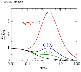
Figure 5: (Color online) Dependence of the diffusion coefficient $D$ given in Eq. (47) on the average waiting time $\tau$ for the extended Poisson walk. The result is presented in dimensionless form for $\sigma_{\text{s}}/\tau_{\text{s}}=1/5$, $\big{(}2/\sqrt{3}-1\big{)}^{1/2}$, $1/\sqrt{3}$, and 1.

V.2 Ratchet as a random walker

Now, we discuss the correspondence between the extended Poisson walker and the ratchet model studied in the preceding section. Let $t$ be the time needed for a particle moving in potential $V_{0}(x)$ given by Eq. (28) to arrive at $x=0$ for the first time provided that it has started at $x=-l$. The probability density function $p(t)$ of $t$ (the first-passage time) is given Hu et al. (2010) by

$$p(t)=\frac{l}{\sqrt{4\pi D_{0}t^{3}}}\exp\left[-\frac{(l-\kappa D_{0}t)^{2}}{4D_{0}t}\right].$$ (50)

The average $\tau_{\text{r}}$ and the variance $\sigma^{2}_{\text{r}}$ of $t$ are calculated from this distribution as

$$\tau_{\text{r}}=l/\kappa D_{0},\quad\sigma^{2}_{\text{r}}=2l/\kappa^{3}D_{0}^{2}.$$ (51)

Note that the same results can be obtained from the closed-form formulas for the moments of the first-passage time; see Ref. Reimann et al. (2002) and Sec. 7 in Ref. Hänggi et al. (1990). It seems reasonable to identify the first-passage time with the stepping time $t_{\text{s}}$ of the walker. Therefore, $\tau_{\text{s}}$ and $\sigma_{\text{s}}$ of the walker should correspond to $\tau_{\text{r}}$ and $\sigma_{\text{r}}$ of the ratchet. The rate $k$ associated with the waiting time of the walker should correspond to the rate of the transition in the ratchet. If the thermal equilibrium of $x$ is achieved before the transition, then this rate is estimated as

$$w=\int_{-\infty}^{\infty}w_{0}^{+}(x)P_{\text{eq}}(x)\,dx=\kappa\omega_{+}/2,$$ (52)

where $P_{\text{eq}}(x)\equiv(\kappa/2)\exp(-\kappa|x|)$ is the equilibrium distribution for the position of a particle in potential $V_{0}(x)$. Identifying $\tau_{\text{r}}$, $\sigma_{\text{r}}^{2}$, and $w$ of the ratchet with $\tau_{\text{s}}$, $\sigma_{\text{s}}$, and $k=1/\tau$ of the walker, respectively, we obtain the same expression for $v$ as Eq. (38) and

$$D=\frac{v^{3}}{\kappa^{3}D_{0}^{2}}\left[1+2\kappa l\left(\frac{D_{0}}{l\omega_{+}}\right)^{2}\right]$$ (53)

from the results (47) for the walker. Equation (53) agrees with Eq. (37) except the second term in the brackets in the latter, which is absent in the former.

The diffusion coefficient (53) obtained for the extended Poisson walk is plotted, in the dimensionless form, against $\tilde{\omega}_{+}=l\omega_{+}/D_{0}$ in Fig. 6, together with the result of Eq. (37) for the ratchet model. We see that the position and the height of the peak of function $\tilde{D}(\tilde{\omega}_{+})$ for the ratchet model agree reasonably well with those of the extended Poisson walk. The peak for the latter model is located at $\tilde{\omega}_{+}=\tilde{\omega}_{+}^{\text{max}}\equiv[\tilde{K}-(\tilde{K}^{2}-6\tilde{K})^{1/2}]/3$ for $\tilde{K}>6$; the peak position approaches unity as $\tilde{\omega}_{+}^{\text{max}}\approx 1+3/2\tilde{K}$ in the limit of large $\tilde{K}$, whereas the peak height increases linearly in $\tilde{K}$ as $\tilde{D}_{\text{max}}\approx 2\tilde{K}/27+1/27$ in the same limit. These expressions are to be compared with Eqs. (40) and (41), respectively. The dependences of $\tilde{\omega}_{+}^{\text{max}}$ and $\tilde{D}_{\text{max}}$, as well as $\tilde{\omega}_{+}^{\text{min}}$ and $\tilde{D}_{\text{min}}$ [which are the values of $\tilde{\omega}_{+}$ and $\tilde{D}$ at the local minimum of $\tilde{D}(\tilde{\omega}_{+})$], on $\tilde{K}$ are shown in Fig. 3(a) and (b), respectively.

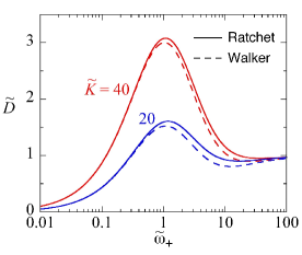
Figure 6: (Color online) Dependence of the diffusion coefficient $\tilde{D}$ on the rate parameter $\tilde{\omega}_{+}$. The result for the ratchet model in the absence of the backward transition, Eq. (37), is shown by the solid line, and that for for the extended Poisson walk, Eq. (53), by the dashed line. The cases of $\tilde{K}=20$ and 40 are presented. The solid lines here are identical to those in Fig. 2(b).

These results demonstrate that the pronounced enhancement of diffusion observed in the ratchet model for large $\tilde{K}$ is well described by the extended Poisson walk. Hence, we suggest that the mechanism for the diffusion enhancement observed in our model of molecular motor is essentially the same as that for the extended Poisson walk; the diffusion is enhanced when the waiting time for the transition is comparable to the time for the particle to slide down the potential slope. Remember that the condition for the diffusion enhancement to occur in the extended Poisson walk is that the fluctuation (the standard deviation) of the stepping time $t_{\text{s}}$ should be somewhat smaller than its average. This condition is satisfied for large $\tilde{K}$ in the ratchet model, since we have $(\sigma_{\text{r}}/\tau_{\text{r}})^{2}=2/\kappa l=2/\tilde{K}$, as can be seen from Eq. (51). This explains why the larger $\tilde{K}$ is, the more salient the diffusion enhancement is.

V.3 A previous model of molecular motors

Let us see if the analogy between a ratchet model and the extended Poisson walk will work for the diffusion enhancement in the previous model of molecular motors Shinagawa and Sasaki (2016), which has some relevance to the F₁-ATPase Kawaguchi et al. (2014). This model is also a potential-switching ratchet described by the Fokker-Planck equation (II), but with different functions for the potential and the transition rates: the potential for and the forward transition rate from “state 0” are given by $V_{0}(x)=Kx^{2}/2$ and $w_{0}^{+}(x)=k\exp(ax)$, respectively, and a constant external force $F$ is applied, where $K$, $k$, and $a$ are positive constants ($k$ is proportional to the ATP concentration). The particle subject to the potential $V_{0}$ and the external force is in mechanical equilibrium at $x=F/K$. Therefore, the average waiting time for the transition from state 0 to state 1 can roughly be estimated as $\tau\sim 1/w_{0}^{+}(F/K)=(1/k)\exp(-aF/K)$. Now, it will take about $\tau_{\text{s}}\sim\gamma/K=k_{\text{B}}T/D_{0}K$ for the particle to slide down on the potential $V_{1}(x)$ from $x=F/K$ to the vicinity of $x=F/K+l$, the mechanical-equilibrium position in state 1, after the transition. Then, Eq. (49) predicts that the diffusion coefficient as a function of $F$ for the motor will be maximized at $F=F_{\text{max}}\sim(K/a)\ln(k_{\text{B}}T/2D_{0}kK)$ with maximum value $D_{\text{max}}\sim 2l^{2}D_{0}K/27k_{\text{B}}T$. These dependences of $F_{\text{max}}$ and $D_{\text{max}}$ on $K$ and $k$ agree within numerical factors with those reported in Ref. Shinagawa and Sasaki (2016) for large $K$ and small $k$ (low ATP concentration). Hence, we think that the mechanism of the diffusion enhancement in molecular motors under low ATP concentrations reported in our previous work Shinagawa and Sasaki (2016) is essentially the same as that in the extended Poisson walk.

VI Concluding Remarks

We have proposed a solvable model of ratchet type for the Brownian motor to elucidate the mechanism underlying the diffusion enhancement reported for a model of molecular motors in our previous work Shinagawa and Sasaki (2016). We have suggested that the diffusion enhancement of the present model observed in a certain range of the transition rate (Sec. IV) and of the previous model Shinagawa and Sasaki (2016) for certain range of external force at low ATP concentrations is essentially the same as the one for a simpler system which we call the extended Poisson walk (Sec. V). In this random walk on a one-dimensional lattice, each step of the walk consists of two processes. One is the Poisson process for the walker to wait on a lattice site, and the other is the stepping to the next site that takes a nonzero time. The enhancement of diffusion occurs when the average waiting time is comparable to the stepping time. In the ratchet model, the waiting time corresponds to the time for the Brownian particle to stay in one potential, and the stepping corresponds to the sliding of the particle on the potential slope after a chemical transition is made.

The analogy between the extended Poisson walk and the ratchet model studied in Sec. IV works only in the limit of small $\omega_{-}$ (the rate of backward transition). Therefore this analogy cannot explain the result presented in Fig. 2(b) that the peak position of the diffusion coefficient as a function of the forward transition rate moves to the right as $\omega_{-}$ increases. Whether this behavior can be understood on the basis of a simple physical picture will be investigated in a future work.

Appendix A Derivation of Eqs. (17) and (18)

To calculate the velocity from the formula (9), we need to obtain the steady-state solutions $P_{n}(x)$ to the Fokker-Planck equations (II). Let $J(x)$ be the function defined by

$$J(x)\equiv\left[f(x)-D_{0}\frac{d}{dx}\right]P(x),$$ (54)

where $P(x)$ is the rescaled $P_{0}(x)$ introduced in Sec. II. Making use of the relation $P_{n}(x)=P_{0}(x-nl)$ and Eq. (5), we obtain

$$\frac{dJ}{dx}=\mathcal{J}\left[\delta(x-a_{-})-\delta(x-a_{+})\right]$$ (55)

with

$$\mathcal{J}\equiv\omega_{+}P(a_{+})-\omega_{-}P(a_{-})$$ (56)

from Eq. (II). Equation (55) implies that $J(x)$ is piecewise constant, and the boundary condition $P(x)\to 0$ as $x\to\pm\infty$ and Eq. (54) suggest that $J(x)\to 0$ as $x\to\pm\infty$. Therefore, Eq. (55) is integrated to yield

$$J(x)=\mathcal{J}\theta(x-a_{-})\theta(a_{+}-x),$$ (57)

where $\theta(x)$ is the step function: $\theta(x)=0$ for $x<0$ and $\theta(x)=1$ for $x\geq 0$. By making use of Eqs. (54) and (57), we can rewrite Eq. (9) as

$$v=\int_{-\infty}^{\infty}J(x)\,dx=\mathcal{J}l.$$ (58)

Substituting Eq. (57) into Eq. (54) and integrating the resulting equation with the boundary condition $P\to 0$ as $|x|\to\infty$, we obtain

$$P(x)=\begin{cases}C_{-}\exp[-U(x)]&(x<a_{-}),\\ \varphi(x)\exp[-U(x)]&(a_{-}\leq x\leq a_{+}),\\ C_{+}\exp[-U(x)]&(x>a_{+}),\end{cases}$$ (59)

where $U(x)$ is defined in Eq. (16), function $\varphi(x)$ is defined by

$$\varphi(x)=C_{-}-\frac{\mathcal{J}}{D_{0}}\int_{a_{-}}^{x}e^{U(y)}\,dy,$$ (60)

and constants $C_{\mp}$ by

$$C_{\mp}=\frac{1+\phi_{0}u_{\pm}/D_{0}}{u_{+}-u_{-}}\mathcal{J}$$ (61)

with $\phi_{0}$ and $u_{\pm}$ defined in Eqs. (13) and (15). We have also used Eq. (56) to get Eq. (61). From Eqs. (58)–(61) we obtain Eqs. (21)–(23).

The expression (59) for $P(x)$ together with Eqs. (60) and (61) contain the unknown constant $\mathcal{J}$. This constant can be determined from the normalization condition (8), which yields

$$\mathcal{J}=\frac{(u_{+}-u_{-})D_{0}}{\zeta(D_{0}+\phi_{0}u_{-})+\phi_{1}(u_{+}-u_{-})},$$ (62)

where $\phi_{1}$ is defined in Eq. (14). From Eqs. (62) and (58) we obtain Eq. (17).

To calculate the diffusion coefficient from the formula (11), we need to solve Eq. (10) to obtain $Q(x)$. Let $L(x)$ be the function defined by

$$L(x)\equiv\left[f(x)-D_{0}\frac{d}{dx}\right]Q(x).$$ (63)

Then, Eq. (10) is rewritten as

$$\frac{dL}{dx} =\lambda\left[\delta(x-a_{-})-\delta(x-a_{+})\right]$$

$$\quad{}+\left[f(x)-v-2D_{0}\frac{d}{dx}\right]P(x)$$ (64)

with

$$\lambda\equiv\omega_{+}Q(a_{+})-\omega_{-}Q(a_{-}).$$ (65)

Taking account of the boundary condition $L(x)\to 0$ as $|x|\to\infty$, which comes from the similar condition for $Q(x)$ and Eq. (63), we integrate Eq. (64) to get

$$L(x)=R(x)+\lambda\theta(x-a_{-})\theta(a_{+}-x),$$ (66)

where $R(x)$ is defined by

$$R(x)\equiv\int_{-\infty}^{x}\left[f(y)-v\right]P(y)\,dy-2D_{0}P(x).$$ (67)

It is convenient to rewrite this expression as follows. From the definition (9) of $f(x)$ and the expression (21) for $P(x)$, we have

$$\int_{-\infty}^{x}f(y)P(y)\,dy=D_{0}P(x)-D_{0}\int_{-\infty}^{x}\frac{dg(y)}{dy}e^{-U(y)}\,dy$$ (68)

by making use of integration by parts. Now, the expression (22) for $g(x)$ is used to rewrite the last term in Eq. (68) as

$$D_{0}\int_{-\infty}^{x}\frac{dg(y)}{dy}e^{-U(y)}\,dy=-vh(x),$$ (69)

where $h(x)$ is defined in Eq. (20). Substitution of Eq. (68) with Eq. (69) into Eq. (67) leads to Eq.(27), i.e.,

$$R(x)=vW(x)-D_{0}P(x)$$ (70)

with $W(x)$ defined in Eq. (19).

Having the function $L(x)$ thus obtained, we substitute Eq. (66) with Eq. (70) into Eq. (63) and integrate the resulting equation to get

$$Q(x)=e^{-U(x)}\left[C-\frac{1}{D_{0}}\int_{a_{-}}^{x}L(y)e^{U(y)}\,dy\right],$$ (71)

where constant $C$ is given by

$$C=\frac{(D_{0}+\phi_{0}u_{+})\lambda+\psi_{0}u_{+}}{(u_{+}-u_{-})D_{0}}$$ (72)

with $\phi_{0}$, $u_{\pm}$, and $\psi_{0}$ defined by Eqs. (13), (15), and (25), respectively. We have also used Eq. (65) to get Eq. (72).

The expression (71) contains the unknown constant $\lambda$ through $C$ given in Eq. (72). This constant cannot be determined uniquely, because $Q(x)$ defined as the solution of Eq. (10) has ambiguity: if $Q(x)$ is a solution of this equation, then $Q(x)+cP(x)$ with $c$ an arbitrary constant is also a solution. However, this ambiguity does not affect the right-hand side of formula (11), since we have

$$\int_{-\infty}^{\infty}\left[f(x)-v\right]P(x)\,dx=0$$

because of the first equation in Eq. (9). Therefore, we can assign any value to $\lambda$. We find it convenient to determine $\lambda$ from the condition

$$\int_{-\infty}^{\infty}Q(x)\,dx=0,$$ (73)

from which we obtain Eq. (24).

Now, we have everything we need to calculate the diffusion coefficient by using the formula (11), which reads

$$D=D_{0}+\int_{-\infty}^{\infty}f(x)Q(x)\,dx$$ (74)

due to Eq. (73). We will rewrite the second term of Eq. (74), because the expression for $Q(x)$ given in Eq. (71) is quite complicated and hence Eq. (74) is not convenient for practical use. First, we use Eqs. (63) and (66) to proceed as

$$\int_{-\infty}^{\infty}f(x)Q(x)\,dx=\int_{-\infty}^{\infty}L(x)\,dx=\lambda l+\int_{-\infty}^{\infty}R(x)\,dx.$$

Next, we use Eq. (70) to obtain Eq. (18).

Appendix B Expressions for $P(x)$ and $W(x)$

Here, we present the explicit expressions for $P(x)$ and $W(x)$ obtained for the model considered in Sec. IV. The steady-state probability density $P(x)$ in state 0 is found to be

$$P(x)=g(x)e^{-\kappa|x|},$$ (75)

where $g(x)=C_{-}$ for $x<-l$,

$$g(x)=C_{-}-\frac{v}{\kappa lD_{0}}\left(e^{\kappa l}-e^{-\kappa x}\right)$$ (76)

for $-l\leq x\leq 0$, and $g(x)=C_{+}$ for $x>0$ with $C_{\pm}$ obtained by substituting Eqs. (29) and (30) into Eq. (23).

The function $W(x)$ defined by Eq. (19) is given by

$$W(x)=\begin{cases}-(C_{-}/\kappa)e^{\kappa x}&(x<-l)\\ (C_{+}/\kappa)e^{-\kappa x}&(x>0)\end{cases}$$ (77)

and

$$W(x)=C_{+}\zeta\left(1+\frac{x}{l}\right)-\frac{C_{-}}{\kappa}e^{\kappa x}+\frac{v}{\kappa^{2}lD_{0}}\left(e^{\kappa(x+l)}-1\right)$$ (78)

for $-l\leq x\leq 0$.