A Framework and Method for Online Inverse Reinforcement Learning

Abstract

Inverse reinforcement learning (IRL) is the problem of learning the preferences of an agent from the observations of its behavior on a task. While this problem has been well investigated, the related problem of online IRL—where the observations are incrementally accrued, yet the demands of the application often prohibit a full rerun of an IRL method—has received relatively less attention. We introduce the first formal framework for online IRL, called incremental IRL (I2RL), and a new method that advances maximum entropy IRL with hidden variables, to this setting. Our formal analysis shows that the new method has a monotonically improving performance with more demonstration data, as well as probabilistically bounded error, both under full and partial observability. Experiments in a simulated robotic application of penetrating a continuous patrol under occlusion shows the relatively improved performance and speed up of the new method and validates the utility of online IRL.

1 Introduction

Inverse reinforcement learning (IRL) [11, 15] refers to the problem of ascertaining an agent’s preferences from observations of its behavior on a task. It inverts RL with its focus on learning the reward function given information about optimal action trajectories. IRL lends itself naturally to a robot learning from demonstrations by a human teacher (often called the expert) in controlled environments, and therefore finds application in robot learning from demonstration [2] and imitation learning [12].

Previous methods for IRL [1, 3, 7, 8, 13, 19] typically operate on large batches of observations and yield an estimate of the expert’s reward function in a one-shot manner. These methods fill the need of applications that predominantly center on imitation learning. Here, the task being performed is observed and must be replicated subsequently. However, newer applications of IRL are motivating the need for continuous learning from streaming data or data in mini-batches. Consider, for example, the task of forecasting a person’s goals in an everyday setting from observing his activities using a body camera [14]. Alternately, a robotic learner observing continuous patrols from a vantage point is tasked with penetrating the patrolling and reaching a goal location speedily and without being spotted [4]. Both these applications offer streaming observations, no episodic tasks, and would benefit from progressively learning and assessing the other agent’s preferences.

In this paper, we present the first formal framework to facilitate investigations into online IRL. The framework, labeled as incremental IRL (I2RL), establishes the key components of this problem and rigorously defines the notion of an incremental variant of IRL. Next, we focus on methods for online IRL. Very few methods exist [10, 14] that are suited for online IRL, and we cast these in the formal context provided by I2RL. More importantly, we introduce a new method that generalizes recent advances in maximum entropy IRL with hidden training data to an online setting. Key theoretical properties of this new method are also established. In particular, we show that the performance of the method improves monotonically with more data and that we may probabilistically bound the error in estimating the true reward after some data both under full observability and when some data is hidden.

Our experiments evaluate the benefit of online IRL on the previously introduced robotic application of penetrating continuous patrols under occlusion [4]. We comprehensively demonstrate that the proposed incremental method achieves a learning performance that is similar to that of the previously introduced batch method. More importantly, it does so in significantly less time thereby suffering from far fewer timeouts and a significantly improved success rate. Consequently, this paper makes important initial contributions toward the nascent problem of online IRL by offering both a formal framework, I2RL, and a new general method that performs well.

2 Background on IRL

Informally, IRL refers to both the problem and method by which an agent learns preferences of another agent that explain the latter’s observed behavior [15]. Usually considered an “expert” in the task that it is performing, the observed agent, say $E$, is modeled as executing the optimal policy of a standard MDP defined as $\langle S_{E},A_{E},T_{E},R_{E}\rangle$. The learning agent $L$ is assumed to perfectly know the parameters of the MDP except the reward function. Consequently, the learner’s task may be viewed as finding a reward function under which the expert’s observed behavior is optimal.

This problem in general is ill-posed because for any given behavior there are infinitely-many reward functions which align with the behavior. Ng and Russell [11] first formalized this task as a linear program in which the reward function that maximizes the difference in value between the expert’s policy and the next best policy is sought. Abbeel and Ng [1] present an algorithm that allows the expert $E$ to provide task demonstrations instead of its policy. The reward function is modeled as a linear combination of $K$ binary features, $\phi_{k}$: $S_{E}\times A_{E}$ $\rightarrow$ $[0,1]$ $,k\in\{1,2\ldots K\}$, each of which maps a state from the set of states $S_{E}$ and an action from the set of $E$’s actions $A_{E}$ to a value in [0,1]. Note that non-binary feature functions can always be converted into binary feature functions although there will be more of them. Throughout this article, we assume that these features are known to or selected by the learner. The reward function for expert $E$ is then defined as $R_{E}(s,a)=\bm{\theta}^{T}\phi(s,a)=\sum_{k=1}^{K}\theta_{k}\cdot\phi_{k}(s,a)$, where $\theta_{k}$ are the weights in vector $\bm{\theta}$; let $\mathcal{R}=\mathbb{R}^{|S_{E}\times A_{E}|}$ be the continuous space of the reward functions. The learner’s task is reduced to finding a vector of weights that complete the reward function, and subsequently the MDP such that the demonstrated behavior is optimal.

To assist in finding the weights, feature expectations are calculated for the expert’s demonstration and compared to those of possible trajectories [19]. A demonstration is provided as one or more trajectories, which are a sequence of length-$T$ state-action pairs, $(\langle s,a\rangle_{1},\langle s,a\rangle_{2},\dots\langle s,a\rangle_{T})$, corresponding to an observation of the expert’s behavior across $T$ time steps. Feature expectations of the expert are discounted averages over all observed trajectories, $\hat{\phi}_{k}=\frac{1}{|X|}\sum_{X\in\mathcal{X}{}}\sum\nolimits_{t=1}^{T}\gamma^{t}~{}\phi_{k}(\langle s,a\rangle_{t})$, where $X$ is a trajectory in the set of all observed trajectories, $\mathcal{X}{}$, and $\gamma\in(0,1)$ is a discount factor. Given a set of reward weights the expert’s MDP is completed and solved optimally to produce $\pi^{*}_{E}$. The difference $\hat{\phi}-\phi^{\pi^{*}_{E}}$ provides a gradient with respect to the reward weights for a numerical solver.

2.1 Maximum Entropy IRL

While expected to be valid in some contexts, the max-margin approach of Abeel and Ng [1] introduces a bias into the learned reward function in general. To address this, Ziebart et al. [19] find the distribution with maximum entropy over all trajectories that is constrained to match the observed feature expectations.

$$\begin{array}[]{l}\max\limits_{\Delta}\left(-\sum\nolimits_{X\in\mathbb{X}}Pr(X)~{}log~{}Pr(X)\right)\\ \\ \mbox{{\bf subject to}}~{}~{}~{}\sum\nolimits_{X\in\mathbb{X}}Pr(X)=1\\ \sum\nolimits_{X\in\mathbb{X}}Pr(X)~{}\sum_{t=1}^{T}\gamma^{t}\phi_{k}(\langle s,a\rangle_{t})=\hat{\phi}_{k}~{}~{}~{}~{}~{}~{}\forall k\end{array}$$ (5)

Here, $\Delta$ is the space of all distributions over the space $\mathbb{X}$ of all trajectories. We denote the analytical feature expectation on the left hand side of the second constraint above as $E_{\mathbb{X}}[\phi_{k}]$.Equivalently, as the distribution is parameterized by learned weights $\bm{\theta}$, $E_{\mathbb{X}}[\phi_{k}]$ represents the feature expectations of policy $\pi^{*}_{E}$ computed using the learned reward function. The benefit is that distribution $Pr(X;\bm{\theta})$ makes no further assumptions beyond those which are needed to match its constraints and is maximally noncommittal to any one trajectory. As such, it is most generalizable by being the least wrong most often of all alternative distributions. A disadvantage of this approach is that it becomes intractable for long trajectories because the set of trajectories grows exponentially with length. In this regard, another formulation defines the maximum entropy distribution over policies [7], the size of which is also large but fixed.

2.2 IRL under Occlusion

Our motivating application involves a subject robot that must observe other mobile robots from a fixed vantage point. Its sensors allow it a limited observation area; within this area it can observe the other robots fully, outside this area it cannot observe at all. Previous methods [4, 5] denote this special case of partial observability where certain states are either fully observable or fully hidden as occlusion. Subsequently, the trajectories gathered by the learner exhibit missing data associated with time steps where the expert robot is in one of the occluded states. The empirical feature expectation of the expert $\hat{\phi}_{k}$ will therefore exclude the occluded states (and actions in those states).

To ensure that the feature expectation constraint in IRL accounts for the missing data, Bogert and Doshi [4] while maximizing entropy over policies [7] limit the calculation of feature expectations for policies to observable states only. A recent approach [6] improves on this method by taking an expectation over the missing data conditioned on the observations. Completing the missing data in this way allows the use of all states in the constraint and with it the Lagrangian dual’s gradient as well. The nonlinear program in (5) is modified to account for the hidden data and its expectation.

Let $Y$ be the observed portion of a trajectory, $Z$ is one way of completing the hidden portions of this trajectory, $\mathbb{Z}$ is the set of all possible $Z$, and $X=Y\cup Z$. Now we may treat $Z$ as a latent variable and take the expectation to arrive at a new definition for the expert’s feature expectations:

$$\hat{\phi}^{Z|_{Y}}_{k}\triangleq\frac{1}{|\mathcal{Y}{}|}\sum\limits_{Y\in\mathcal{Y}}\sum\limits_{Z\in\mathbb{Z}}Pr(Z|Y;\bm{\theta})\sum\nolimits_{t=1}^{T}\gamma^{t}\phi_{k}(\langle s,a\rangle_{t})$$ (6)

where $\langle s,a\rangle_{t}\in Y\cup Z$, $\mathcal{Y}{}$ is the set of all observed $Y$ and $\mathcal{X}{}$ is the set of all complete trajectories. The program in (5) is modified by replacing $\hat{\phi}_{k}$ with $\hat{\phi}^{Z|_{Y}}_{k}$, as we show below. Notice that in the case of no occlusion $\mathbb{Z}$ is empty and $\mathcal{X}{}=\mathcal{Y}{}$. Therefore $\hat{\phi}^{Z|_{Y}}_{k}=\hat{\phi}_{k}$ and this method reduces to (5). Thus, this method generalizes the previous maximum entropy IRL method.

$$\begin{array}[]{l}\max\limits_{\Delta}\left(-\sum\nolimits_{X\in\mathbb{X}}Pr(X)~{}log~{}Pr(X)\right)\\ \\ \mbox{{\bf subject to}}~{}~{}~{}\sum\nolimits_{X\in\mathbb{X}}Pr(X)=1\\ \sum\nolimits_{X\in\mathbb{X}}Pr(X)~{}\sum_{t=1}^{T}\gamma^{t}\phi_{k}(\langle s,a\rangle_{t})=\hat{\phi}^{Z|_{Y}}_{k}~{}~{}~{}~{}~{}~{}\forall k\end{array}$$ (11)

However, the program in (11) becomes nonconvex due to the presence of $Pr(Z|Y)$. As such, finding its optima by Lagrangian relaxation is not trivial. Wang et al. [18] suggests a log linear approximation to obtain maximizing $Pr(X)$ and casts the problem of finding the reward weights as likelihood maximization that can be solved within the schema of expectation-maximization [9]. An application of this approach to the problem of IRL under occlusion yields the following two steps with more details in [6]:

E-step This step involves calculating Eq. 6 to arrive at $\hat{\phi}^{Z|_{Y},(t)}_{k}$, a conditional expectation of the $K$ feature functions using the parameter $\bm{\theta}^{(t)}$ from the previous iteration. We may initialize the parameter vector randomly.

M-step In this step, the modified program (11) is optimized by utilizing $\hat{\phi}^{Z|_{Y},(t)}_{k}$ from the E-step above as the expert’s constant feature expectations to obtain $\bm{\theta}^{(t+1)}$. Normalized exponentiated gradient descent [16] solves the program.

As EM may converge to local minima, this process is repeated with random initial $\bm{\theta}$ and the solution with the maximum entropy is chosen as the final one.

3 Incremental IRL (I2RL)

We present our framework labeled I2RL in order to realize IRL in an online setting. Then, we present an initial set of methods cast into the framework of I2RL. In addition to including previous techniques for online IRL, we introduce a new method that generalizes the maximum entropy IRL involving latent variables.

3.1 Framework

Expanding on the notation and definitions given previously in Section 2, we introduce some new notation, which will help us in defining I2RL rigorously.

Definition 1 (Set of fixed-length trajectories).

The set of all trajectories of finite length $T$ from an MDP attributed to the expert $E$ is defined as, $\mathbb{X}^{T}=\{X|X=(\langle s,a\rangle_{1},\langle s,a\rangle_{2},\ldots\langle s,a\rangle_{T}),\forall s\in S_{E},\forall a\in A_{E}\}$.

Let $\mathbb{N}^{+}$ be a bounded set of natural numbers. Then, the set of all trajectories is $\mathbb{X}={\mathbb{X}^{1}\cup\mathbb{X}^{2}\cup\ldots\cup\mathbb{X}^{|\mathbb{N}^{+}|}}$. Recall that a demonstration is some finite set of trajectories of varying lengths, $\mathcal{X}{}=\{X^{T}|X^{T}\in\mathbb{X}^{T},T\in\mathbb{N}^{+}\}$, and it includes the empty set.  Subsequently, we may define the set of demonstrations.

Definition 2 (Set of demonstrations).

The set of demonstrations is the set of all subsets of the spaces of trajectories of varying lengths. Therefore, it is the power set, $2^{\mathbb{X}}=2^{\mathbb{X}^{1}\cup\mathbb{X}^{2}\cup\ldots\cup\mathbb{X}^{|\mathbb{N}^{+}|}}$.

In the context of the definitions above, traditional IRL attributes an MDP without the reward function to the expert, and usually involves determining an estimate of the expert’s reward function, $\hat{R}_{E}\in\mathcal{R}$, which best explains the observed demonstration, $\mathcal{X}{}\in 2^{\mathbb{X}}$. As such, we may view IRL as a function: $\zeta(MDP_{/R_{E}},\mathcal{X}{})=\hat{R}_{E}$.

To establish the definition of I2RL, we must first define a session of I2RL. Let $\hat{R}^{0}_{E}$ be an initial estimate of the expert’s reward function.

Definition 3 (Session).

A session of I2RL represents the following function: $\zeta_{i}(MDP_{/R_{E}},\mathcal{X}{}_{i},\hat{R}^{i-1}_{E})=\hat{R}^{i}_{E}$. In this $i^{th}$ session where $i>0$, I2RL takes as input the expert’s MDP sans the reward function, the demonstration observed since the previous session, $\mathcal{X}{}_{i}\in 2^{\mathbb{X}}$, and the reward function estimate learned from the previous session. It yields a revised estimate of the expert’s rewards from this session of IRL.

Note that we may replace the reward function estimates with some statistic that is sufficient to compute it (e.g., $\bm{\theta}$).

We may let the sessions run infinitely. Alternately, we may establish stopping criteria for I2RL, which would allow us to automatically terminate the sessions once the criterion is satisfied. Let $LL(\hat{R}_{E}^{i}|\mathcal{X}{}_{1:i})$ be the log likelihood of the demonstrations received up to the $i^{th}$ session given the current estimate of the expert’s reward function. We may view this likelihood as a measure of how well the learned reward function explains the observed data.

Definition 4 (Stopping criterion #1).

Terminate the sessions of I2RL when $|LL(\hat{R}_{E}^{i}|\mathcal{X}{}_{1:i})-LL(\hat{R}_{E}^{i-1}|\mathcal{X}{}_{1:i-1})|\leqslant\epsilon$, where $\epsilon$ is a very small positive number and is given.

Definition 4 reflects the fact that additional sessions are not impacting the learning significantly. On the other hand, a more effective stopping criterion is possible if we know the expert’s true policy. We utilize the inverse learning error [8] in this criterion, which gives the loss of value if $L$ uses the learned policy on the task instead of the expert’s: $ILE(\pi^{*}_{E},\pi_{E}^{L})=||V^{\pi^{*}_{E}}-V^{\pi_{E}^{L}}||_{1}$. Here, $V^{\pi^{*}_{E}}$ is the optimal value function of $E$’s MDP and $V^{\pi_{E}^{L}}$ is the value function due to utilizing the learned policy $\pi_{E}^{L}$ in $E$’s MDP. Notice that when the learned reward function results in an identical optimal policy to $E$’s optimal policy, $\pi^{*}_{E}=\pi_{E}^{L}$, ILE will be zero; it increases monotonically as the two policies increasingly diverge in value.

Definition 5 (Stopping criterion #2).

Terminate the sessions of I2RL when $ILE(\pi^{*}_{E},\pi_{E}^{i-1})-ILE(\pi^{*}_{E},\pi_{E}^{i})\leqslant\epsilon$, where $\epsilon$ is a very small positive error and is given. Here, $\pi_{E}^{i}$ is the optimal policy obtained from solving the expert’s MDP with the reward function $\hat{R}_{E}^{i}$ learned in session $i$.

Obviously, prior knowledge of the expert’s policy is not common. Therefore, we view this criterion as being more useful during the formative assessments of I2RL methods.

Utilizing Defs. 3, 4, and 5, we formally define I2RL next.

Definition 6 (I2RL).

Incremental IRL (I2RL) is a sequence of learning sessions $\{\zeta_{1}(MDP_{/R_{E}},\mathcal{X}{}_{1},\hat{R}^{0}_{E}),\zeta_{2}(MDP_{/R_{E}},\mathcal{X}{}_{2},\hat{R}^{1}_{E}),\zeta_{3}(MDP_{/R_{E}},\mathcal{X}{}_{3},\hat{R}^{2}_{E}),\ldots,\}$, which continue infinitely, or until either stopping criterion #1 or #2 is met depending on which one is chosen a’priori.

3.2 Methods

Our goal is to facilitate a portfolio of methods each with its own appealing properties under the framework of I2RL. This would enable online IRL in various applications. An early method for online IRL [10] modifies Ng and Russell’s linear program [11] to take as input a single trajectory (instead of a policy) and replaces the linear program with an incremental update of the reward function. We may easily present this method within the framework of I2RL. A session of this method $\zeta_{i}(MDP_{/R_{E}},\mathcal{X}{}_{i},\hat{R}_{E}^{i-1})$ is realized as follows: Each $\mathcal{X}{}_{i}$ is a single state-action pair $\langle s,a\rangle$; initial reward function $\hat{R}_{E}^{0}=\frac{1}{\sqrt{|S_{E}|}}$, whereas for $i>0$ $\hat{R}_{E}^{i}=\hat{R}_{E}^{i-1}+\alpha\cdot v_{i}$, where $v_{i}$ is the difference in expected value of the observed action $a$ at state $s$ and the (predicted) optimal action obtained by solving the MDP with the reward function $\hat{R}_{E}^{i-1}$, and $\alpha$ is the learning rate. While no explicit stopping criterion is specified, the incremental method terminates when it runs out of observed state-action pairs. Jin et al. [10] provide the algorithm for this method as well as error bounds.

A recent method by Rhinehart and Kitani [14] performs online IRL for activity forecasting. Casting this method to the framework of I2RL, a session of this method is $\zeta_{i}(MDP_{/R_{E}},\mathcal{X}{}_{i},\bm{\theta}^{i-1})$, which yields $\bm{\theta}^{i}$. Input observations for the session, $\mathcal{X}{}_{i}$, are all the activity trajectories observed since the end of previous goal until the next goal is reached. The session IRL finds the reward weights $\bm{\theta}^{i}$ that minimize the margin $\phi^{\pi^{*}_{E}}-\hat{\phi}$ using gradient descent. Here, the expert’s policy $\pi^{*}_{E}$ is obtained by using soft value iteration for solving the complete MDP that includes a reward function estimate obtained using previous weights $\bm{\theta}^{i-1}$. No explicit stopping criterion is utilized for the online learning thereby emphasizing its continuity.

3.2.1 Incremental Latent MaxEnt

We present a new method for online IRL under the I2RL framework, which modifies the latent maximum entropy (LME) optimization of Section 2.2. It offers the capability to perform online IRL in contexts where portions of the observed trajectory may be occluded.

For differentiation, we refer to the original method as the batch version. Recall the $k^{th}$ feature expectation of the expert computed in Eq. 6 as part of the E-step. If $X_{i}=Y_{i}\cup Z_{i}$ is a trajectory in session $i$ composed of the observed portion $Y_{i}$ and the hidden portion $Z_{i}$, $\hat{\phi}^{Z|_{Y},1:i}_{k}$ is the expectation computed using all trajectories obtained so far, we may rewrite Eq. 6 for feature $k$ as:

$$\hat{\phi}^{Z|_{Y},1:i}_{k} \triangleq\frac{1}{|\mathcal{Y}{}_{1:i}|}\sum\limits_{Y\in\mathcal{Y}{}_{1:i}}\sum\limits_{Z\in\mathbb{Z}}Pr(Z|Y;\bm{\theta})\sum\limits_{t=1}^{T}\gamma^{t}\phi_{k}(\langle s,a\rangle_{t})$$

$$=\frac{1}{|\mathcal{Y}{}_{1:i}|}\left(\sum\limits_{Y\in\mathcal{Y}{}_{1:i-1}}\sum\limits_{Z\in\mathbb{Z}}Pr(Z|Y;\bm{\theta})\sum\limits_{t=1}^{T}\gamma^{t}\phi_{k}(\langle s,a\rangle_{t})+\sum\limits_{Y\in\mathcal{Y}{}_{i}}\sum\limits_{Z\in\mathbb{Z}}Pr(Z|Y;\bm{\theta})\sum\limits_{t=1}^{T}\gamma^{t}\phi_{k}(\langle s,a\rangle_{t})\right)$$

$$=\frac{1}{|\mathcal{Y}{}_{1:i}|}\left(|\mathcal{Y}{}_{1:i-1}|~{}\hat{\phi}^{Z|_{Y},1:i-1}_{k}+|\mathcal{Y}{}_{i}|~{}\hat{\phi}^{Z|_{Y},i}_{k}\right)~{}~{}~{}~{}~{}~{}~{}~{}~{}~{}~{}~{}~{}~{}~{}~{}~{}~{}~{}~{}~{}~{}(\text{by definition})$$

$$=\frac{|\mathcal{Y}{}_{1:i-1}|}{|\mathcal{Y}{}_{1:i-1}|+|\mathcal{Y}{}_{i}|}~{}\hat{\phi}^{Z|_{Y},1:i-1}_{k}+\frac{|\mathcal{Y}{}_{i}|}{|\mathcal{Y}{}_{1:i-1}|+|\mathcal{Y}{}_{i}|}~{}\hat{\phi}^{Z|_{Y},i}_{k}$$ (12)

A session of our incremental LME takes as input the expert’s MDP sans the reward function, the current session’s trajectories, the number of trajectories observed until the start of this session, the expert’s empirical feature expectation and reward weights from previous session. More concisely, each session is denoted by, $\zeta_{i}(MDP_{/R_{E}},\mathcal{Y}{}_{i},|\mathcal{Y}_{1:i-1}|,\hat{\phi}^{Z|_{Y},1:i-1},\bm{\theta}^{i-1})$. In each session, the feature expectations using that session’s observed trajectories are computed, and the output feature expectations are obtained by including these as shown above in Eq. 12. Of course, each session may involve several iterations of the E- and M-steps until the converged reward weights $\bm{\theta}^{i}$ is obtained thereby giving the corresponding reward function estimate. Here, the expert’s feature expectation is a sufficient statistic to compute the reward function. We refer to this method as LME I2RL.

Wang et al. [17] shows that if the distribution over the trajectories in (11) is log linear, then the reward function that maximizes the entropy of the trajectory distribution also maximizes the log likelihood of the observed portions of the trajectories. Given this linkage with log likelihood, the stopping criterion #1 as given in Def. 4 is utilized. In other words, the sessions will terminate when, $|LL(\bm{\theta}^{i}|\mathcal{Y}{}_{1:i})-LL(\bm{\theta}^{i-1}|\mathcal{Y}{}_{1:i-1})|\leq\epsilon$, where $\bm{\theta}^{i}$ fully parameterizes the reward function estimate from the $i^{th}$ session and $\epsilon$ is a given acceptable difference. The algorithm for this method is presented in the supplementary file.

Incremental LME admits some significant convergence guarantees with a confidence of meeting the desired error-specification on the demonstration likelihood. We state these results with discussions but defer the detailed proofs to the supplementary file.

Lemma 1 (Monotonicity).

Incremental LME increases the demonstration likelihood monotonically with each new session, $LL(\bm{\theta}^{i}|\mathcal{Y}{}_{1:i})-LL(\bm{\theta}^{i-1}|\mathcal{Y}{}_{1:i-1})\geqslant 0$, when $|\mathcal{Y}{}_{1:i-1}|\gg|\mathcal{Y}{}_{i}|$, yielding a feasible solution to I2RL with missing training data.

While Lemma 1 suggests that the log likelihood of the demonstration can only improve from session to session after a significant amount of training data has been accumulated, a stronger result illuminates the confidence with which it approaches, over a series of sessions, the log likelihood of the expert’s true weights $\bm{\theta}_{E}$. To establish this convergence result, we first focus on the full observability setting. For a desired bound $\varepsilon$ on the log-likelihood loss (difference in likelihood w.r.t expert’s $\bm{\theta}_{E}$ and that w.r.t learned $\bm{\theta}^{i}$) for session $i$ in this setting, the confidence is bounded as follows:

Theorem 1 (Confidence for incremental max-entropy IRL).

Given $\mathcal{X}{}_{1:i}$ as the (fully observed) demonstration till session $i$, $\bm{\theta}_{E}\in[0,1]^{K}$ is the expert’s weights, and $\bm{\theta}^{i}$ is the solution of session $i$ for incremental max-entropy IRL, we have

$$LL(\bm{\theta}_{E}|\mathcal{X}{}_{1:i})-LL(\bm{\theta}^{i}|\mathcal{X}{}_{1:i})\leqslant\varepsilon$$

with probability at least $1-\delta$, where $\delta=2K\exp\left[-\frac{|\mathcal{X}{}_{1:i}|\varepsilon^{2}(1-\gamma)^{2}}{2K^{2}}\right]$.

As a step toward relaxing the assumption of full observability made above, we first consider the error in approximating the feature expectations of the unobserved portions of the data, accumulated from the first to the current session of I2RL. Notice that $\hat{\phi}^{Z|_{Y},1:i}_{k}$ given by Eq. 12, is an approximation of the full-observability expectation $\hat{\phi}^{1:i}_{k}$, estimated by sampling the hidden $Z$ from $Pr(Z|Y,\bm{\theta}^{i-1})$ [6]. The following lemma relates the error due to this sampling-based approximation, i.e., $\left|\hat{\phi}^{1:i}_{k}-\hat{\phi}^{Z|_{Y},1:i}_{k}\right|$, to the difference between feature expectations for learned policy and that estimated for the expert’s true policy.

Lemma 2 (Constraint Bounds for incremental LME ).

Suppose $\mathcal{X}{}_{1:i}$ has portions of trajectories in $\mathbb{Z}_{1:i}=\{Z|(Y,Z)\in\mathcal{X}{}_{1:i}\}$ occluded from the learner. Let $\varepsilon_{sampling}$ be a bound on the error $\left|\hat{\phi}^{1:i}_{k}-\hat{\phi}^{Z|_{Y},1:i}_{k}\right|_{1},k\in\{1,2\ldots K\}$ after $N$ samples for approximation. Then, with probability at least $1-(\delta+\delta_{sampling})$, the following holds:

$$\left|E_{\mathbb{X}}[\phi_{k}]-\hat{\phi}^{Z|_{Y},1:i}_{k}\right|_{1}\leqslant\varepsilon/2K+\varepsilon_{sampling},k\in\{1,2\ldots K\}$$

where $\varepsilon,\delta$ are as defined in Theorem 1, and $\delta_{sampling}=2K\exp(-2(1-\gamma)^{2}(\varepsilon_{sampling})^{2}N)$.

Theorem 1 combined with Lemma 2 now allows us to completely relax the assumption of full observability as follows:

Theorem 2 (Confidence for incremental LME).

Let $\mathcal{Y}_{1:i}=\{Y|(Y,Z)\in\mathcal{X}{}_{1:i}\}$ be the observed portions of the demonstration until session $i$, $\varepsilon,\varepsilon_{sampling}$ are inputs as defined in Lemma 2, and $\bm{\theta}^{i}$ is the solution of session $i$ for incremental LME, then we have

$$LL(\bm{\theta}_{E}|\mathcal{Y}{}_{1:i})-LL(\bm{\theta}^{i}|\mathcal{Y}{}_{1:i})\leq\varepsilon_{latent}$$

with a confidence at least $1-\delta_{latent}$, where $\varepsilon_{latent}=\varepsilon+2K\varepsilon_{sampling}$, and $\delta_{latent}=\delta+\delta_{sampling}$.

Given required inputs and fixed $\varepsilon_{latent}$, Theorem  2 computes a confidence $1-\delta_{latent}$. The amount of required demonstration, $|\mathcal{Y}_{1:i}|$, can be decided based on the desired magnitude of the confidence.

4 Experiments

We evaluate the benefit of online IRL on the perimeter patrol domain, introduced by Bogert and Doshi [4], and simulated in ROS using data and files made publicly available. It involves a robotic learner observing two guards continuously patrol a hallway as shown in Fig. 1(left). The learner is tasked with reaching the cell marked ’X’ (Fig. 1(right)) without being spotted by any of the patrollers. Each guard can see up to 3 grid cells in front. This domain differs from the usual applications of IRL toward imitation learning. In particular, the learner must solve its own distinct decision-making problem (modeled as another MDP) that is reliant on knowing how the guards patrol, which can be estimated from inferring each guard’s preferences. The guards utilized two types of binary state-action features leading to a total of six: does the current action in the current state make the guard change its grid cell? And, is the robot’s current cell $(x,y)$ in a given region of the grid, which is divided into 5 regions? The true weight vector $\bm{\theta}_{E}$ for these feature functions is $\langle.57,0,0,0,.43,0\rangle$.

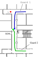
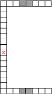
Figure 1: The map and corresponding MDP state space for each patroller [4]. Shaded squares are the turn-around states and the red ’X’ is $L$’s goal state. $L$ is unaware of where each patroller turns around or their navigation capabilities.

Notice that the learner’s vantage point limits its observability. Therefore, this domain requires IRL under occlusion. Among the methods discussed in Section 2, LME allows IRL when portions of the trajectory are hidden, as mentioned previously. To establish the benefit of I2RL, we compare the performances of both batch and incremental variants of this method.

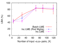
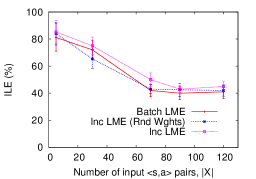
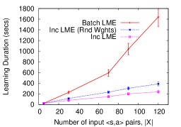
(a) Learned behavior accuracy, ILE, and learning duration under a 30% degree of observability.

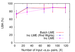
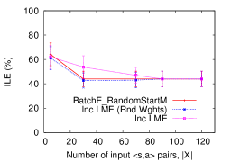
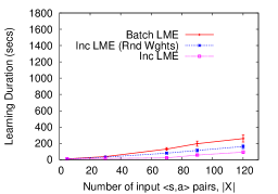
(b) Learned behavior accuracy, ILE, and learning duration under a 70% degree of observability.

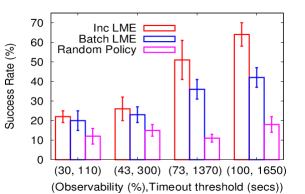
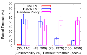
(c) Success rates and timeouts under both 30%, 70%, and full observability. The success rate obtained by a random baseline is shown as well. This method does not perform IRL and picks a random time to start moving to the goal state.

Figure 2: Various metrics for comparing the performances of batch and incremental LME on Bogert and Doshi’s [4] perimeter patrolling domain. Our experiments were run on a Ubuntu 16 LTS system with an Intel i5 2.8GHz CPU core and 8GB RAM.

Efficacy of the methods was compared using the following metrics: learned behavior accuracy (LBA), which is the percentage of overlap between the learned policy’s actions and demonstrated policy’s actions; ILE, which was defined previously in Section 3.1; and success rate, which is the percentage of runs where $L$ reaches the goal state undetected. Note that when the learned behavior accuracy is high, we expect ILE to be low. However, as MDPs admit multiple optimal policies, a low ILE need not translate into a high behavior accuracy. As such, these two metrics are not strictly correlated.

We report the LBA, ILE, and the time duration in seconds of the inverse learning for both batch and incremental LME in Figs. 2$(a)$ and 2$(b)$; the latter under a 30% degree of observability and the former under 70%. Each data point is averaged over 100 trials for a fixed degree of observability and a fixed number of state-action pairs in the demonstration $\mathcal{X}{}$. While the entire demonstration is given as input to the batch variant, the $\mathcal{X}{}_{i}$ for each session has one trajectory. As such, the incremental learning stops when there are no more trajectories remaining to be processed. To better understand any differentiations in performance, we introduce a third variant that implements each session as, $\zeta_{i}(MDP_{/R_{E}},\mathcal{Y}{}_{i},|\mathcal{Y}_{i:i-1}|,\hat{\phi}^{Z|_{Y},1:i-1})$. Notice that this incremental variant does not utilize the previous session’s reward weights, instead it initializes them randomly in each session; we label it as incremental LME with random weights.

As the size of demonstration increases, both batch and incremental variants exhibit similar quality of learning although initially the incremental performs slightly worse. Importantly, incremental LME achieves these learning accuracies in significantly less time compared to batch, with the speed up ratio increasing to four as $|\mathcal{X}{}|$ grows.

Is there a benefit due to the reduced learning time? We show the success rates of the learner when each of the three methods are utilized for IRL in Fig. 2$(c)$. Incremental LME begins to demonstrate comparatively better success rates under 30% observability itself, which further improves when the observability is at 70%. While the batch LME’s success rate does not exceed 40%, the incremental variant succeeds in reaching the goal location undetected in about 65% of the runs under full observability (the last data point). A deeper analysis to understand these differences reveals that batch LME suffers from a large percentage of timeouts – more than 50% for low observability, which drops down to 10% for full observability. A timeout occurs when IRL fails to converge to a reward estimate in the given amount of time for each run. On the other hand, incremental LME suffers from very few timeouts. Of course, other factors play a role in success as well.

5 Concluding Remarks

This paper makes an important contribution toward the nascent problem of online IRL by offering the first formal framework, I2RL, to help analyze the class of methods for online IRL. We presented a new method within the I2RL framework that generalizes recent advances in maximum entropy IRL to online settings. Our comprehensive experiments show that the new I2RL method indeed improves over the previous state-of-the-art in time-limited domains, by approximately reproducing its accuracy but in significantly less time. In particular, we have shown that given practical constraints on computation time for an online IRL application, the new method suffers fewer timeouts and is thus able to solve the problem with a higher success rate. In addition to experimental validation, we have also established key theoretical properties of the new method, ensuring the desired monotonic progress within a pre-computable confidence of convergence. Future avenues for investigation include understanding how I2RL can address some of the challenges related to scalability to a larger number of experts as well as the challenge of accommodating unknown dynamics of the experts.

References

- [1] P. Abbeel and A. Y. Ng. Apprenticeship learning via inverse reinforcement learning. In Twenty-first International Conference on Machine Learning (ICML), pages 1–8, 2004.
- [2] B. D. Argall, S. Chernova, M. Veloso, and B. Browning. A survey of robot learning from demonstration. Robotics and autonomous systems, 57(5):469–483, 2009.
- [3] M. Babes-Vroman, V. Marivate, K. Subramanian, and M. Littman. Apprenticeship learning about multiple intentions. In 28th International Conference on Machine Learning (ICML), pages 897–904, 2011.
- [4] K. Bogert and P. Doshi. Multi-robot inverse reinforcement learning under occlusion with state transition estimation. In International Conference on Autonomous Agents and Multiagent Systems (AAMAS), pages 1837–1838, 2015.
- [5] K. Bogert and P. Doshi. Toward estimating others’ transition models under occlusion for multi-robot irl. In 24th International Joint Conference on Artificial Intelligence (IJCAI), pages 1867–1873, 2015.
- [6] K. Bogert, J. F.-S. Lin, P. Doshi, and D. Kulic. Expectation-maximization for inverse reinforcement learning with hidden data. In 2016 International Conference on Autonomous Agents and Multiagent Systems, pages 1034–1042, 2016.
- [7] A. Boularias, O. Krömer, and J. Peters. Structured apprenticeship learning. In European Conference on Machine Learning and Knowledge Discovery in Databases, Part II, pages 227–242, 2012.
- [8] J. Choi and K.-E. Kim. Inverse reinforcement learning in partially observable environments. J. Mach. Learn. Res., 12:691–730, 2011.
- [9] A. P. Dempster, N. M. Laird, and D. B. Rubin. Maximum likelihood from incomplete data via the em algorithm. Journal of the Royal Statistical Society, Series B (Methodological), 39:1–38, 1977.
- [10] Z. jun Jin, H. Qian, S. yi Chen, and M. liang Zhu. Convergence analysis of an incremental approach to online inverse reinforcement learning. Journal of Zhejiang University - Science C, 12(1):17–24, 2010.
- [11] A. Ng and S. Russell. Algorithms for inverse reinforcement learning. In Seventeenth International Conference on Machine Learning, pages 663–670, 2000.
- [12] T. Osa, J. Pajarinen, G. Neumann, J. A. Bagnell, P. Abbeel, and J. Peters. An algorithmic perspective on imitation learning. Foundations and Trends® in Robotics, 7(1-2):1–179, 2018.
- [13] D. Ramachandran and E. Amir. Bayesian inverse reinforcement learning. In 20th International Joint Conference on Artifical Intelligence (IJCAI), pages 2586–2591, 2007.
- [14] N. Rhinehart and K. M. Kitani. First-person activity forecasting with online inverse reinforcement learning. In International Conference on Computer Vision (ICCV), 2017.
- [15] S. Russell. Learning agents for uncertain environments (extended abstract). In Eleventh Annual Conference on Computational Learning Theory, pages 101–103, 1998.
- [16] J. Steinhardt and P. Liang. Adaptivity and optimism: An improved exponentiated gradient algorithm. In 31st International Conference on Machine Learning, pages 1593–1601, 2014.
- [17] S. Wang, R. Rosenfeld, Y. Zhao, and D. Schuurmans. The Latent Maximum Entropy Principle. In IEEE International Symposium on Information Theory, pages 131–131, 2002.
- [18] S. Wang and D. Schuurmans Yunxin Zhao. The Latent Maximum Entropy Principle. ACM Transactions on Knowledge Discovery from Data, 6(8), 2012.
- [19] B. D. Ziebart, A. Maas, J. A. Bagnell, and A. K. Dey. Maximum entropy inverse reinforcement learning. In 23rd National Conference on Artificial Intelligence - Volume 3, pages 1433–1438, 2008.