Learning Device Models with Recurrent Neural Networks

Abstract

Recurrent neural networks (RNNs) are powerful constructs capable of modeling complex systems, up to and including Turing Machines. However, learning such complex models from finite training sets can be difficult. In this paper we empirically show that RNNs can learn models of computer peripheral devices through input and output state observation. This enables automated development of functional software-only models of hardware devices. Such models are applicable to any number of tasks, including device validation, driver development, code de-obfuscation, and reverse engineering. We show that the same RNN structure successfully models six different devices from simple test circuits up to a 16550 UART serial port, and verify that these models are capable of producing equivalent output to real hardware.

I Introduction

In this paper we consider whether RNNs can learn functionally equivalent models of unknown computer hardware peripherals through input/output observation. Peripheral devices attach to a main computer and use both hardware within the device and driver software running on the main computer to perform a task, such as printing a page or sending a message. However, there are instances when hardware is accessible from the main system but driver software is not, rendering the peripheral unusable. This situation is prevalent in open source operating systems where driver software may not be available from the vendor. Without driver software or development documentation, it is incumbent on the system’s owner to write software to make use of the peripheral. The device itself is a “black box”, with no information directly available to the developer beyond a set of memory addresses to interact with the device and the observable output of the hardware itself. This leads to labor-intensive reverse engineering efforts with varying degrees of success (see e.g. [1]). Ideally, future adaptable systems should be able to automatically probe, observe, and develop models of unknown devices to either inform the development process, or write interface software directly. Such solutions would also be useful in the areas of evolutionary robotics [2] and hardware validation [3] [4].

Traditional automated black box learning techniques which learn exact models, such as L* [5] or TTT [6], are prohibitively expensive for this task since computer peripherals have large input and output spaces, a large number of internal states, and require a complex series of commands to perform a task. Alternatively, Recurrent Neural Networks (RNNs) offer an intriguing solution to peripheral device modelling as they are able to learn approximate models without the computational overhead required for traditional techniques. RNNs are versatile and powerful constructs that add memory to traditional feed-forward neural networks via backwards (or loop) connections from output layers to previous layers. RNNs are capable of modeling Turing Machines [7]. Recent advances in machine learning hardware and software allow powerful, multi-layer RNNs to be trained efficiently.

The central scientific contribution of this paper is an empirical study of the effectiveness of using RNNs to model computer peripheral devices. We include a dataset of simple machines that mimic real device behavior (Section IV), and then compare how well RNNs model those machines. Our experiments show (Section V) that RNNs are capable of learning functionally-equivalent models of simple hardware devices, and lay the groundwork for future adaptable systems.

II Problem Statement and Assumptions

We approach the problem of learning device models as a black box learning problem. Each device $D$ has the ability to accept a sequence of input commands $I$, such as writes to a command register or memory-mapped addresses, which in turn produce a sequence of observable outputs $O$, such as data on a wire or lights on the device. Our goal is to learn an approximate functional model $M$ of the device $D$ such that $D-M<\epsilon$, such that $\epsilon$ is minimized. $D-M$ is expressed in this work as the observed functional difference (or loss) between $D$’s response to input $I$ and $M$’s response to the same input.

We assume no knowledge of the inner workings of the device being modeled. We assume that the learning algorithm either has access to a set of observations of the device, or has the ability to generate such a set. We also assume that the observed output sequence of a device is in some way influenced by the input sequence, which we believe is a reasonable assumption for most peripherals. Finally, we assume that the set of observations for the device contains at least some characteristic traces that exercise a significant portion of the device’s capability. These assumptions will not hold true for all potential scenarios, and indeed learning complete models from black box systems is known to be infeasible in the general case, but we assert they should hold for a significantly large subset of target peripherals.

III Related Work

The first area of related work is the area of black box automata learning techniques. Black box automata learning has two main approaches: active and passive learning. Angluin [5] proposed the $L^{*}$ active learning algorithm which can infer a Mealy machine given the presence of an oracle who knows the real state machine. Variations of this algorithm are in use today [8] [6], and are applied to such areas as hardware and software component testing [9], formal model verification [10], hardware reverse engineering [4], and network protocol inference [11]. Recently, work has begun on learning register automata, which allows a memory stack within the learned automata [12], which may improve performance.

In passive learning, it is infeasible to actively query the device under test so the learner is limited to the set of input and output sequences previously gathered from the device. Gold [13] produced early work in this field, showing that inferring a minimal Moore Machine from examples was NP-Complete [14]. Passive learning algorithms descended from Gold’s work include RPNI [15], OSTIA [16], and MooreMI [17].

Automata learning approaches such as those above suffer from their need to learn complete and accurate (though not necessarily minimal) representations of the systems under test. In general, the complexity of active learning grows linearly with the number of inputs and quadratically with the number of states [18]. Thus, active learning is only tractable for small problems, or large problems that can be broken down into smaller problems ahead of time by an expert with domain knowledge. Passive learning in general is known to be NP-Complete. The work in this paper aims to overcome these limitations on black box algorithms by using RNNs to learn approximate models that are close enough to the real models to be functionally equivalent.

Two related areas of RNN research include using RNNs or RNN-like structures to model computing systems, such as the Neural Turing Machine [19] and Zaremba and Sutskever [20] who train neural networks with memory to perform computation; and automata extraction from trained neural networks. Examples of extraction methods for feed-forward networks include FERNN [21], DeepRED [22], and HYPINV [23]. More recent examples targeting RNNs include Murdoch and Szlam [24], and Weiss, et al. [25].

IV Experimental Setup

To test the ability of RNNs to learn models from devices, we created a set of simulated devices that perform actions which mimic those of real hardware peripherals. The simulated devices contain interesting state transitions that test how well an RNN is able to learn complex concepts yet are simple enough for manual verification of the results. These simulated test devices are shown in Figure 1.

IV-A Simple Machines

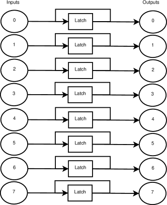
(a) EightBitMachine

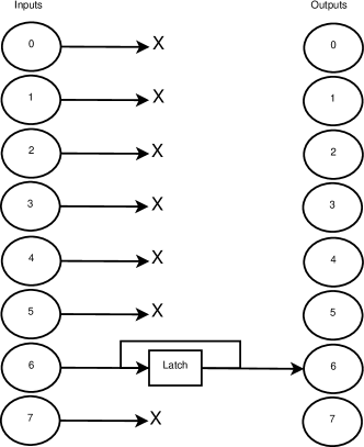
(b) SingleDirectMachine

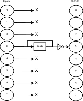
(c) SingleInvertMachine

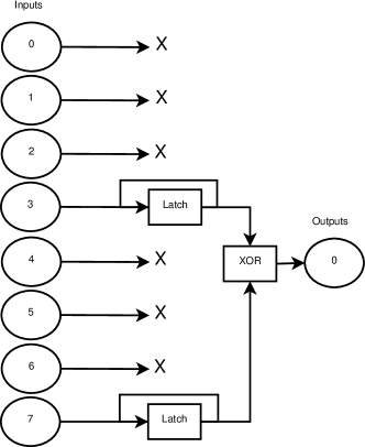
(d) SimpleXORMachine

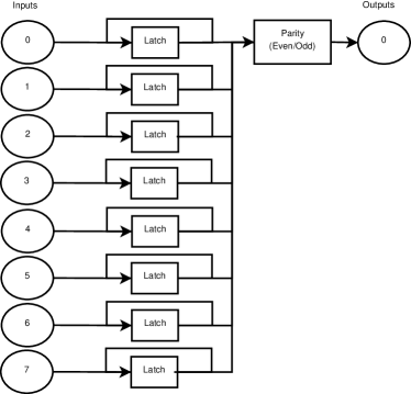
(e) ParityMachine

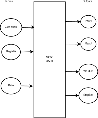
(f) SerialPortMachine

Figure 1: Simulated machines of increasing complexity used for testing. All inputs are latched, meaning they retain the latest written value for all subsequent commands.

We define a set of five simple artificial machines described below in order of increasing complexity. In each machine the inputs are latched, meaning that setting an input to a value of $1$ or $0$ can have an effect on future outputs depending on the internal structure of the machine. In these machines, the input value is stored in memory, and remains the same for future commands in the sequence until explicitly changed.

• EightBitMachine: A simple mapping of 8 inputs to 8 outputs.

• SingleDirectMachine: 7 inputs are ignored and one leads directly to a single output.

• SingleInvertMachine: Same as a above, but output is inverted.

• SimpleXORMachine: 6 inputs are ignored, and the remaining two are XOR’d together to produce the single output.

• ParityMachine: The output is set to $1$ if an odd number of inputs are set, and $0$ if an even number are set.

An evaluation of the magnitude of the state spaces of these machines is available in Appendix A. These simple models provide an easily decomposable testing ground to test what RNNs can learn about a machine. Success in modeling these devices will provide confidence that the RNN will be able to handle more complex systems in the future.

IV-B 16550 UART

While the simple models detailed above test the basic ability of RNNs to learn discrete concepts used by devices, the 16550 UART model shows a practical application of the RNN approach to a real world peripheral. The 16550 UART [26] is the component behind the modern PC serial port and communicates using the RS-232 serial communications standard [27]. The device is controlled via a series of commands written to 8 8-bit registers. These registers control the desired communications parameters, notably baud rate, word length, parity, and the number of stop bits used when sending or receiving data. The device then either listens for incoming data, or the programmer writes data to the transmit register which is transmitted over the serial bus using the configured parameters. Table I shows the set of possible values for each output state used in our software model.

Setting	Values	Description
Word Length	5,6,7,8 bits	Size of the data to send
Baud Rate	Value between 0-115200	Base wire clock rate
Stop Bits	1, 1.5, 2 bits	End-of-frame bits
Parity	None,Odd,Even,High,Low	Meaning of parity bits
TX Data	Value 0-255	Data to transmit

TABLE I: Relevant RS-232 settings with descriptions

The 16550 UART peripheral makes a good, complex use case for model learning for several reasons:

• Relevance: The 16550 UART is used in many systems today because it is simple enough for even the most basic operating systems to control.

• Hidden Registers: The device has 12 internal registers mapped to 8 register addresses. The learner must discover how to access all registers before it can change some states.

• Output Interdependence: Certain outputs can only be observed if other outputs are set to specific values. For example, a setting of 1.5 stop bits can only happen if the word length is 5.

• Diverse Output Types: Some observable outputs can take on one of a small set of values, but the baud rate is a single value from a set of $2^{16}-1$ possible values, and the data transmitted over the wire is drawn from $2^{8}$ values.

• Hidden Mathematical Formula: The baud rate is determined via an inherent mathematical formula of 115200 divided by the concatenated value of two other registers. The learner will have to discover this hidden constant to accurately model the device.

Many devices have traits similar to the above. Our simulated 16550 machine simulates register inputs and their meanings at the bit level. It simulates data transmission only, read commands are recognized but return no data, as there is no simulated peer from which to receive data. While limited, this software model is sufficient to simulate the interesting complexities of a UART detailed above. If a RNN can model a 16550 UART accurately then that is a good indication that it can successfully model more complex devices.

IV-C Generating Observations

We generated a uniform random set of input sequences for each simulated machine under test, ran those through each machine and recorded the corresponding output set to create a dataset of observations used to train the RNN. Random sampling of the input space is not ideal, but is sufficient for this experiment as it represents a worst case scenario versus a more intelligent sampling scheme.

For the simple machines, the input sequences consisted of a tuple of a ’set’ or ’clear’ command, and the number of the input to modify. The output is the vector of results from the machine, with each output bit set to $1.0$ or $0.0$, representing if the bit was set or cleared. See Figure 2 for a detailed example of a command sequence and its input and output encoding. For the 16550 UART, the input sequences are a tuple of command, register, and data; where command is either ’read’ or ’write’, register is the offset of the register to act upon, and data is the 8-bit value to write (it is ignored for read commands). The output of the machine is the state of each output specified in Table I, with parity, stop bits, and word length encoded as one-hot entries; baud rate encoded as a scaled floating point value between $0.0$ and $1.0$; a single output flag that determines whether data was transmitted at that time step; and if so, the data transmitted encoded as 8 binary digits. See Figure 3 for an example encoding of a sequence.

Figure 2: Example command sequence with encoding for EightBitMachine. The input and output for the sequence is encoded as a 2-dimensional floating point array.

Figure 3: Example command sequence with encoding for SerialPortMachine. Note that parity, word length, and stop bits are one-hot encoded, data is binary encoded, baud rate is linearly scaled between 0 and 1, and the transmit flag is True/False.

Using the above encodings, we generated 4096 training sequences, 1024 validation sequences used during training, and a separate set of 128 sequences used for evaluation after training is complete. Each training, validation, and evaluation sequence contains 1024 commands.

IV-D Recurrent Neural Network

Our experimental RNNs are multi-layer neural networks consisting of GRU [28] cells. Early experiments confirmed that non-recurrent networks were unable to learn models of these systems. Both GRU and LSTM [29] cells were considered, and while both were able to learn these models, networks with GRU cells trained faster and were more stable. The same network structure is used for each test case to make sure that the same method will work regardless of the underlying device. The basic structure is shown in Figure 4, with four hidden layers and an activation function $f$ after each GRU cell. Each layer is fully connected to its neighbors.

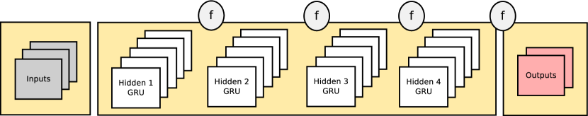
Figure 4: Neural network structure learning device models. The width of each hidden layer is chosen to be larger than the maximum size of either the input or output layer.

Each hidden layer has more cells than the maximum width of either the input or the output layers. The experiments shown here use the heuristic $max(I_{width},O_{width})+1$ to determine the number of recurrent cells in each hidden layer. This allows the network to learn the model without artificial pressure to compress its internal representation. This heuristic does create over-sized networks when there are large disparities between the input and output widths which we speculate could lead to overfitting and memorization, although that was not observed in these experiments.

The number of hidden layers was determined experimentally. Early tests showed that two hidden layers was sufficient to learn models of all test machines except ParityMachine. Expanding the network to four hidden recurrent layers allowed this basic network structure to learn models for all test machines considered.

V Results

We divide the experimental results into two sets. The first set is the aggregated results of training a large number of networks for each test machine to verify that learning is taking place. We compare each network’s output to the validation dataset’s output, and verify that the difference between the two, or validation loss, is both decreasing with training time, and achieves a small value in a reasonable amount of time.

The second set of results pushes even further and tests whether, with continued training, a RNN can exactly model the behavior of a real device at every time step. This requires not only achieving a low validation loss, but also accurate results when presented with previously unknown inputs.

V-A Successful Learning

We trained 50 recursive networks with the training and validation dataset sequences for each machine type using Keras [30] with the TensorFlow [31] backend, for a total of 300 different network instances. The full set of parameters used for training is covered in Appendix B.

Each network was trained until the validation loss for the model dropped below $0.1\%$ ($0.001$) for more than 20 consecutive epochs, or a maximum of 4096 epochs, whichever came first. When training was complete, each network was evaluated further by computing the difference between predicted and expected output on the previously-unseen evaluation dataset. The average evaluation loss among all networks of a particular type is shown in Table II. A network is considered “successfully trained” if the loss on the evaluation dataset is less than $5\%$, a threshold chosen to show that significant learning had occurred even if the network failed to achieve the stopping criteria of $0.1\%$. Experiments in the next section will determine if either threshold is sufficient to accurately mimic the underlying device’s output. By this criteria, the ParityMachine type proved hardest to learn, with only 78% of the test networks successfully trained, while all other machine types achieved successful learning in $98\%$ of instances or higher.

Machine	# Params	Epochs	% Success	Eval Loss
EightBitMachine	2,461	231	98%	0.002515
SingleDirectMachine	2,461	206	98%	0.003003
SingleInvertMachine	2,461	37	100%	0.000018
SimpleXORMachine	2,384	155	98%	0.002466
ParityMachine	2,384	1875	78%	0.023999
SerialPortMachine	10,398	773	98%	0.003326

TABLE II: Results of training 50 networks for each machine

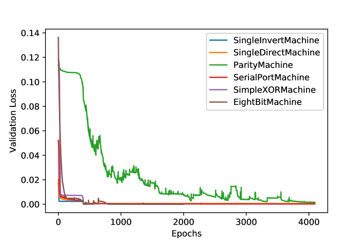
Figure 5: Average validation loss per epoch using only the networks that successfully trained for each machine type.

Figure 5 shows the average validation loss per epoch for each machine type. This shows that most machine types, on average, approach our terminal value of $0.1\%$ validation loss within the first 100 epochs, with the notable exception of ParityMachine, which often takes hundreds or thousands of epochs before terminating, if it learns at all. The SerialPortMachine type in particular is much more complex than the others yet still converges quickly, indicating RNNs can model a large subset of devices.

RNNs are susceptible to unpredictability caused by random weight initialization. Despite attempts to control all other variables, we still observe variability in the success rate and learning performance of each individual network. For example, Figure 6 shows the complete set of successful validation loss performances for each of the 50 trained networks for the EightBitMachine type. As shown, the majority of networks started with a loss between $15\%$ and $20\%$, and achieved less than $0.1\%$ loss by epoch 100. There are three outliers; one which starts off much better and finishes in less than 30 epochs, one that gets stuck around $12\%$ error until epoch 400, and one that gets stuck at $12\%$ error, and then fluctuates wildly until it finally converges near epoch 2000. Similar patterns re-occur for each machine type. This indicates it is necessary to train multiple instances in parallel to guarantee good learning performance.

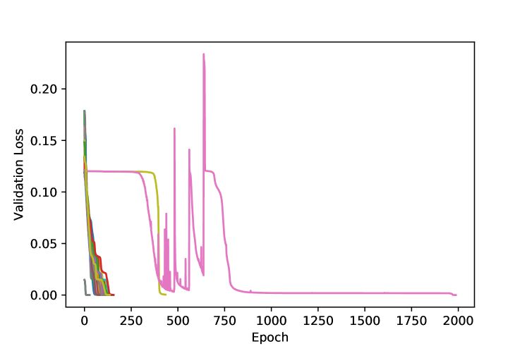
Figure 6: Validation loss for each of 50 trained EightBitMachine networks

V-B Real-World Effectiveness

Having shown that learning is possible for each machine type, the next set of results explore how accurately the learned RNN model can mimic the behavior of the original device. This is different than calculating the global loss over the output sequence because the network is returning an encoded floating-point representations of predictions on each output using the encoding scheme described in Sections IV-A and IV-B. The predicted output sequences for each network need to be converted back to their original output values (via rounding, in most cases) to properly mimic the output of the original machine.

To evaluate model effectiveness, we choose one of the successful RNNs from the previous set of results at random, and continue training it until it is capable of accurately modelling the evaluation dataset for the underlying machine. This means that every output, at every time step, must be identical to that of the original machine. The results of this experiment are shown in Table III. The number of outputs for each machine indicates the total number of outputs the network must correctly predict for 128 evaluation instances, which is output vector width * sequence length (1024) * number of instances (128). The number of extra epochs of training required to hit the highpoint of accuracy is shown under “Epochs+”, while “Epochs” is the total number of epochs required to achieve the result. Training halted when the network achieved complete accuracy on the evaluation dataset for 20 consecutive epochs.

Machine	# Outputs	Epochs	Epochs+	Accuracy
EightBitMachine	1048576	210	57	100%
SingleDirectMachine	1048576	28	0	100%
SingleInvertMachine	1048576	69	40	100%
ParityMachine	131072	4026	1939	99.9992%
SimpleXORMachine	131072	83	21	100%
SerialPortMachine	2883584	N/A	33000+	N/A

TABLE III: Maximum evaluation accuracy with output mapping.

These results clearly show that a low validation loss in training does not always translate into perfect real-world performance. While it is true that the SingleDirectMachine did not require any more training to achieve perfect evaluation accuracy, every other machine required more epochs to approach that goal. Two models were unable to achieve 100% accuracy. The ParityMachine type was able to correctly predict all but one output correctly with 1939 additional epochs, but was unable to move beyond that value despite letting the experiment run for several thousand more epochs. Given the observed variability in learning this particular machine, we expect a 100% accurate ParityMachine model is possible.

The SerialPortMachine type was also unable to achieve perfect mimicry by continuing training on this test, despite having a global error loss approaching $2*10^{-5}$. This model is complex, with 22 values in its output vector representing 6 different values. We continued to train the SerialPortMachine instance for over 33000 extra instances, but failed to achieved perfect accuracy on the evaluation dataset. Table IV shows the results of a simple ”Hello World!” command sequence at three different settings for the network at approximately 33000 epochs. We can observe that while the Word Length, Parity, and Stop Bits settings are correctly predicted, the Baud rate and Data outputs are far less accurate.

Target	Baudrate	Wordlen	Parity	Sbits	Output
115200,8n1	115285	8	None	1	Haxxo Wofxp!
9600,7e1	1936	7	Even	1	Haxxo Wofxp!
2400,7o2	853	7	Odd	2	Haxxo Wofxp!

TABLE IV: Example ”Hello World!” output after 33,000+ epochs, single network

To determine why, we first examine which outputs are contributing the most to the error. Figure 7 shows validation loss heatmaps of each output at different stages of training. Each cell represents the loss of a particular output value (x-axis) for each command in the 1024-command evaluation sequence (y-axis). Darker colors mean the value at that output is closer to the correct value within the sequence. We show three maps, one towards the beginning of training, and two more as training continues. We note the evolution of the training over time, and observe the overall loss approaching $0.0$. But while the Parity, Word Length, and Stop Bits outputs significantly decreased their loss over time, the data transmitted and baud rate are the most difficult for the network to learn.

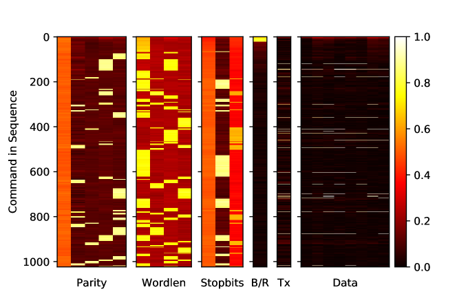
(a) 16 Epochs, $10\%$ Global Loss

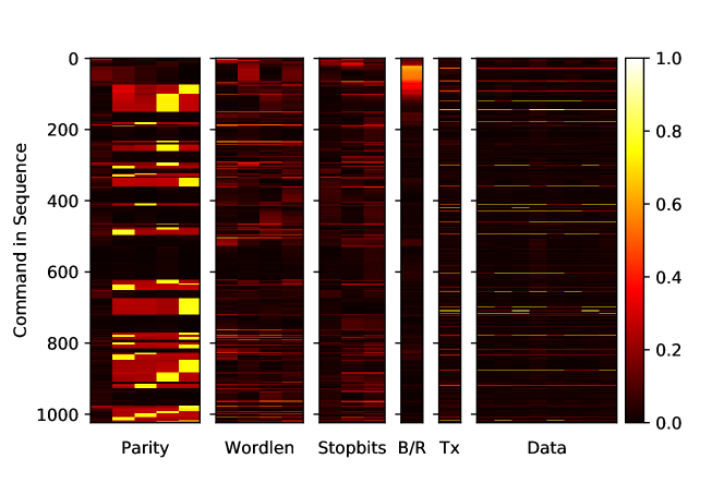
(b) 176 Epochs, $2.7\%$ Global Loss

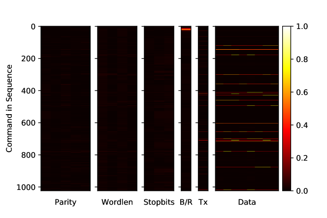
(c) 2640 Epochs $0.29\%$ Global Loss

Figure 7: Local error sources contributing to global error for an example evaluation sequence of 1024 commands issued to a successful UART model.

We speculate this is for a few reasons. First, the baud rate can take any one of $2^{16}$ possible values, and is encoded as a single 32-bit floating point number. Thus, the network must predict the value to within $1.0/2^{16}=1.5*10^{-5}$ to be correct. This may be just too difficult for the network to do accurately. Future work will use a different encoding for this value. Second, due to randomly generating commands for training data, the number of commands in a sequence that actually transmit data is small compared to the number of commands overall. Thus, we speculate that learning the data outputs is hard due to a low proportion of data transmit commands in the command sequence.

V-C Decomposed Model

We speculate a further contributing negative factor to 100% accuracy with the SerialPortMachine is that the value the network is optimizing for is the global loss over that instance. The SerialPortMachine type has $22*1024=22528$ outputs per instance, nearly three times as large as any other tested machine. With this large output space, even small amounts of noise or error from each cell mask where the network needs to minimize the real error. To test this theory, we created a new model made up of multiple neural networks, one for each output type: Parity, Word Length, Stop Bits, Baud Rate, Tx, and Data. We call this a decomposed model, as it decomposes the problem into smaller networks. Intuitively, if the network only has to optimize for one output type it may be able to learn faster, as it is optimizing over fewer outputs.

Output	Encoding	Output Size	Epochs	Val. Loss
Parity	one-hot	5	579	$5.4*10^{-6}$
Word Length	one-hot	4	340	$1.2*10^{-5}$
Stop Bits	one-hot	3	251	$2.7*10^{-5}$
Baud Rate	float	1	1260	$1.2*10^{-4}$
Tx	true/false	1	322	$2.3*10^{-5}$
Data	binary	8	628	$1.1*10^{-5}$

TABLE V: Characteristics of decomposed model networks for UART

We are careful to use the same network structure as when training with all outputs in one network, and only change the width of the output layer. The 16550 UART outputs are not always independent, so the network must model all possible states even if it is only predicting one. Therefore it is important to keep the same hidden layer widths from the non-decomposed network to avoid state compression pressure when training the decomposed models.

Target	Baudrate	Wordlen	Parity	Sbits	Output
115200,8n1	115199	8	None	1	H!llo wop,d!
9600,7e1	2210	7	Even	1	Hello w/rld!
2400,7o2	146	7	Odd	2	Hello w/rld!

TABLE VI: Example ”Hello World!” output, multiple networks

Metadata about these networks is shown in Table V, including how long each took to reach the stopping criteria and the validation loss at that time. The result of the example “Hello World” from before is shown in Table VI. While still not able to achieve 100% accuracy, the decomposed model is significantly better at predicting the final data transmitted, and trains in much less time than training the entire model at once.

VI Discussion

These results show that recurrent neural networks can be trained to learn information about the inner workings of black box devices. For the simple test machines, the results are very accurate, and while the UART model was not able to precisely learn all outputs, it was able to accurately model several components of the system and make progress towards the remainder. We are confident that perfect accuracy on all models is achievable.

It is important to note that the structure of the networks used for each machine type is identical. With expert knowledge, one could create network structures tailored for a specific target machine, but this generic structure shows that modeling can be successful without specific knowledge of the underlying machine. Thus, this method is applicable to a wide range of use cases.

These results suggest that minor tweaks can be made to the methods presented here to achieve even more accurate results in the future. While true, the experimental results here are sufficient to support the notion that RNNs are useful tools for modeling systems like computer peripherals.

Furthermore, compared to traditional black box methods like L*, RNNs are able to model more complex systems. State of the art black box systems can only accurately model devices with a few hundred unique internal states. While our simple test machines have up to $2^{8}$ possible internal states, real devices like the 16550 UART has on the order of $2^{37}$ possible internal states (See Appendix A. Such systems are simply too complex to learn with traditional black box algorithms.

The observed difficulty in learning a larger, complex systems like the UART suggests that global output loss may not be the optimal parameter to optimise for, as the larger the number of outputs and the longer the sequence, the less impact each individual output has on that value. Our decomposed model is able to overcome this issue for our test case, delivering better results within a fraction of the time.

Finally, we note that the observed validation loss highlights the difficulty of knowing when to terminate training. Some networks had long periods of little to no improvement in validation loss, only to suddenly learn the model hundred or even thousands of epochs later.

VII Future Work

We plan to expand testing to include peripheral devices which utilize large memory maps, such as VGA text mode, or DMA and interrupts, such as a simple network card. The UART model is being improved to generate and interpret raw RS-232 waveforms to infer settings and data, as opposed to the current software model which simply supplies that information at each time step. This leads to interesting learning challenges as the same waveform can map to multiple meanings, introducing ambiguity in the training data. This will also allow the learned models to interact with physical UART devices.

Further research is needed into output encodings and their impact on learning. The baud rate, encoded as floating point, appeared to be the hardest for the networks to learn, so different encoding techniques will be explored to quantify the practical limits on regression accuracy when predicting floating point values.

Future work will also focus on efficient methods to extract the learned automata from the neural network. This will allow automated documentation and explanation of unknown peripherals to the user.

VIII Conclusions

This paper shows empirically that RNNs are capable of modeling even complex real-world devices accurately using single, generic network structure. In addition, we introduced a sample test machine dataset useful for evaluating other techniques for modeling peripheral devices. With time, we hope the technique can be improved and combined with automata extraction to gain unprecedented insight into the inner workings of unknown peripherals.

Appendix A Machine State Spaces

Each machine has an input state space, and output state space, and an internal state space. The input state space is the number of possible valid inputs, the output state space is the number of possible valid outputs, and the internal state space is the number of possible internal states the machine can represent at a time. The magnitude of the state space of each machine for a single command is shown in Table VII.

Machine	Input	Output	Internal
EightBitMachine	$2^{9}$	$2^{8}$	$2^{8}$
SingleDirectMachine	$2^{9}$	$2^{1}$	$2^{1}$
SingleInvertMachine	$2^{9}$	$2^{1}$	$2^{1}$
SimpleXORMachine	$2^{9}$	$2^{1}$	$2^{2}$
ParityMachine	$2^{9}$	$2^{1}$	$2^{8}$
SerialPortMachine	$2^{12}$	$2^{37}$	$2^{37}$

TABLE VII: Approximate magnitude of state spaces for each machine.

Appendix B Keras Parameters

The full list of Keras RNN hyperparameters used for the experiments in this paper is shown in Table VIII. A full analysis of how these parameters were chosen is outside the scope of this paper, but they were chosen empirically via sampling the hyperparameter search space. Some alternative options are shown in the Options column. The hyperparameter that had the most impact on modelling success was the choice of activation function. The experiments in this paper use tanh as the activation function as it provided the most consistent and accurate results with a low probability of instability during training. The selu function also performed well. Interestingly, the similar sigmoid activation function performed poorly in nearly all early experiments, as did the relu family of functions. Dropout and other regularization techniques were not enabled, as over-fitting was not observed in these experiments.

Parameter	Value	Options
Layer Type	GRU	GRU,LSTM,SimpleRNN,Dense
Activation Function	tanh	tanh,linear,(s)elu,sigmoid,relu
Optimizer	nadam	adam,nadam,rmsprop,sgd
Loss Function	msle	msle,mse,mape
# Hidden Layers	4	1,2,4 or 8

TABLE VIII: Keras hyper-parameters used for experiments

References

- [1] M. Peres, “Nouveau - recap, on-going and future work,” free and Open Source Software Developers’ European Meeting (FOSDEM) 2012. [Online]. Available: http://phd.mupuf.org/files/fosdem2012_slides.pdf
- [2] Y. Chen, J. Tůmová, and C. Belta, “LTL robot motion control based on automata learning of environmental dynamics,” in 2012 IEEE International Conference on Robotics and Automation, pp. 5177–5182.
- [3] P. Lutsky, “Automating testing by reverse engineering of software documentation,” in , Proceedings of 2nd Working Conference on Reverse Engineering, 1995, pp. 8–12.
- [4] G. Chalupar, S. Peherstorfer, E. Poll, and J. d. Ruiter, “Automated reverse engineering using lego.” [Online]. Available: https://www.usenix.org/conference/woot14/workshop-program/presentation/chalupar
- [5] D. Angluin, “Learning regular sets from queries and counterexamples,” vol. 75, no. 2, pp. 87–106. [Online]. Available: http://linkinghub.elsevier.com/retrieve/pii/0890540187900526
- [6] M. Isberner, F. Howar, and B. Steffen, “The ttt algorithm: A redundancy-free approach to active automata learning.” in RV, 2014, pp. 307–322.
- [7] H. T. Siegelmann and E. D. Sontag, “Turing computability with neural nets,” vol. 4, no. 6, pp. 77–80, 00299. [Online]. Available: http://www.sciencedirect.com/science/article/pii/089396599190080F
- [8] M. J. Kearns and U. V. Vazirani, An introduction to computational learning theory. MIT press, 1994.
- [9] A. Groce, D. Peled, and M. Yannakakis, “Adaptive model checking,” in International Conference on Tools and Algorithms for the Construction and Analysis of Systems. Springer, 2002, pp. 357–370.
- [10] D. Peled, M. Y. Vardi, and M. Yannakakis, “Black box checking,” in Formal Methods for Protocol Engineering and Distributed Systems. Springer, 1999, pp. 225–240.
- [11] G. Bossert, F. Guihéry, G. Hiet et al., “Netzob: un outil pour la rétro-conception de protocoles de communication,” in SSTIC 2012, 2012, p. 43.
- [12] F. Aarts, B. Jonsson, and J. Uijen, “Generating models of infinite-state communication protocols using regular inference with abstraction,” in IFIP International Conference on Testing Software and Systems. Springer, 2010, pp. 188–204.
- [13] E. Gold, “System identification via state characterization,” vol. 8, no. 5, pp. 621–636. [Online]. Available: http://dx.doi.org/10.1016/0005-1098(72)90033-7
- [14] E. M. Gold, “Complexity of automaton identification from given data,” vol. 37, no. 3, pp. 302–320. [Online]. Available: http://www.sciencedirect.com/science/article/pii/S0019995878905624
- [15] J. Oncina and P. García, “Identifying regular languages in polynomial time,” Advances in Structural and Syntactic Pattern Recognition, vol. 5, no. 99-108, pp. 15–20, 1992.
- [16] J. Oncina, P. García, and E. Vidal, “Learning subsequential transducers for pattern recognition interpretation tasks,” IEEE Transactions on Pattern Analysis and Machine Intelligence, vol. 15, no. 5, pp. 448–458, 1993.
- [17] G. Giantamidis and S. Tripakis, “Learning moore machines from input-output traces,” in FM 2016: Formal Methods: 21st International Symposium, Limassol, Cyprus, November 9-11, 2016, Proceedings 21. Springer, pp. 291–309, 00001. [Online]. Available: http://link.springer.com/chapter/10.1007/978-3-319-48989-6_18
- [18] F. Vaandrager, “Model learning,” Communications of the ACM, vol. 60, no. 2, pp. 86–95, 2017.
- [19] A. Graves, G. Wayne, and I. Danihelka, “Neural turing machines,” 00244. [Online]. Available: http://arxiv.org/abs/1410.5401
- [20] W. Zaremba and I. Sutskever, “Learning to execute.” [Online]. Available: http://arxiv.org/abs/1410.4615
- [21] R. Setiono and W. K. Leow, “Fernn: An algorithm for fast extraction of rules from neural networks,” Applied Intelligence, vol. 12, no. 1-2, pp. 15–25, 2000.
- [22] J. R. Zilke, E. L. Mencia, and F. Janssen, “DeepRED – rule extraction from deep neural networks,” in Discovery Science. Springer, Cham, pp. 457–473. [Online]. Available: https://link.springer.com/chapter/10.1007/978-3-319-46307-0_29
- [23] E. W. Saad and D. C. Wunsch, “Neural network explanation using inversion,” Neural Networks, vol. 20, no. 1, pp. 78–93, 2007.
- [24] W. J. Murdoch and A. Szlam, “Automatic rule extraction from long short term memory networks,” 00000. [Online]. Available: http://arxiv.org/abs/1702.02540
- [25] G. Weiss, Y. Goldberg, and E. Yahav, “Extracting Automata from Recurrent Neural Networks Using Queries and Counterexamples.” [Online]. Available: https://arxiv.org/abs/1711.09576
- [26] T. Instruments, “Pc16550d universal asynchronous receiver/transmitter with fifos,” 1995. [Online]. Available: http://www.ti.com/lit/ds/symlink/pc16550d.pdf
- [27] “TIA-232: Interface Between Data Terminal Equipment and Data Circuit-Terminating Equipment Employing Serial Binary Data Interchange rev. f,” Telecommunications Industry Association, Arlington, VA, US, Standard, Oct. 1997.
- [28] K. Cho, B. Van Merriënboer, D. Bahdanau, and Y. Bengio, “On the properties of neural machine translation: Encoder-decoder approaches,” arXiv preprint arXiv:1409.1259, 2014.
- [29] S. Hochreiter and J. Schmidhuber, “Long short-term memory,” Neural Comput., vol. 9, no. 8, pp. 1735–1780, Nov. 1997. [Online]. Available: http://dx.doi.org/10.1162/neco.1997.9.8.1735
- [30] F. Chollet, “Keras,” https://github.com/fchollet/keras, 2015.
- [31] M. Abadi, A. Agarwal, P. Barham, E. Brevdo, Z. Chen, C. Citro, G. S. Corrado, A. Davis, J. Dean, M. Devin, S. Ghemawat, I. Goodfellow, A. Harp, G. Irving, M. Isard, Y. Jia, R. Jozefowicz, L. Kaiser, M. Kudlur, J. Levenberg, D. Mané, R. Monga, S. Moore, D. Murray, C. Olah, M. Schuster, J. Shlens, B. Steiner, I. Sutskever, K. Talwar, P. Tucker, V. Vanhoucke, V. Vasudevan, F. Viégas, O. Vinyals, P. Warden, M. Wattenberg, M. Wicke, Y. Yu, and X. Zheng, “TensorFlow: Large-scale machine learning on heterogeneous systems,” 2015, software available from tensorflow.org. [Online]. Available: https://www.tensorflow.org/