MOABB: Trustworthy algorithm benchmarking for BCIs

Abstract

BCI algorithm development has long been hampered by two major issues: Small sample sets and a lack of reproducibility. We offer a solution to both of these problems via a software suite that streamlines both the issues of finding and preprocessing data in a reliable manner, as well as that of using a consistent interface for machine learning methods. By building on recent advances in software for signal analysis implemented in the MNE toolkit, and the unified framework for machine learning offered by the scikit-learn project, we offer a system that can improve BCI algorithm development. This system is fully open-source under the BSD licence and available at https://github.com/NeuroTechX/moabb. To validate our efforts, we analyze a set of state-of-the-art decoding algorithms across 12 open access datasets, with over 250 subjects. Our analysis confirms that different datasets can result in very different results for identical processing pipelines, highlighting the need for trustworthy algorithm benchmarking in the field of BCIs, and further that many previously validated methods do not hold up when applied across different datasets, which has wide-reaching implications for practical BCIs.

I Introduction

Brain-computer interfaces (BCIs) have long presented the neuroscience methods community with a unique challenge. Unlike in vision research, where one has a database of images and labels, a BCI is defined by a signal recorded from the brain and fed into a computer, which can be influenced in any number of ways both by the subject and by the experimenter. As a result, validating approaches has always been a difficult task. Number of channels, requested task, physical setup, and many other features vary between the numerous publically available datasets online, not to mention issues of convenience such as file format and documentation. Because of this, the BCI methods community has long done one of two things to validate an new approach: Recorded a new dataset, or used one of few well-known, tried-and-true datasets.

Recording a new dataset, the ideal way to show that a proposed method works in practice, presents problems for post-hoc analysis. Without making data public, it is impossible to know whether offline classification results are convincing or due to some coding issue or recording artifact. Further, it is well-known that differences in hardware [28, 21], paradigm [2], and subject [2] can have large differences in the outcome of a BCI task, making it very difficult to generalize findings from any single dataset.

Over the years many datasets have been published online, and serve as an attractive option when time or hardware do not permit recording a new one. In the last year and a half, over a thousand journal and conference submissions have been written on the BCI Competition III [5, 27] and IV [32] datasets. Considering that these datasets have been available publically for over a decade, the true number of papers which validate results against them is likely much higher. While it is impossible to deny the impact these two datasets have had on the field, relying so heavily on a small number of datasets – with less than 50 subjects total – exposes the field to several important issues. In particular, overfitting to the setups offered there is likely.

Lastly, and possibly most problematically, the scarcity of available code for BCI algorithms old and new puts the onus on each individual lab to reproduce the code for all other competing methods in order to make a claim to be comparable with the ’state-of-the-art’ (SOA). As a result, the vast majority of novel BCI algorithm papers compare either against other work from the same lab, or old, easily implementable standards such as CSP [19] or channel-level variances combined with a classifier of choice [12].

Computer vision has solved this problem with enormous datasets like Imagenet [10] bundled with machine learning packages (Tensorflow[1], PyTorch, and Theano[23]). However, generating BCI data is often a very taxing process both physically and mentally, and so it is not reasonable to create datasets of such size. Rather, the field requires many different people recording data in many contexts in order to create an appropriate benchmark. We propose our platform, the MOABB (Mother Of All BCI Benchmarks) Project, as a candidate for this application. The MOABB project consists of the aggregation of many publicly available EEG datasets, converted to a common format and bundled in the software package, as well as a collection of SOA algorithms. Using this system researchers can to automatically benchmark those algorithms and run an automated statistical analysis, making the process of validating new algorithms painless and reproducible. The source code is written in Python and publically available under the BSD licence at https://github.com/NeuroTechX/moabb.

As an initial validation of this project, we present results on the constrained task of binary classification in two-class imagined motor imagery, as that is the most widely used motor imagery paradigm and allows us to demonstrate the process across the largest number of datasets. However, we note that this is only the first question we attempt to answer in this field. The format allows for many other questions, including different channel types (EEG, fNIRS, or other), multi-class paradigms, and also transfer learning scenarios as described in [17].

II Methods

Any BCI analysis is defined by three elements: A dataset, a context, and a pipeline. Here we describe how all of these components are dealt with within our framework, and how specifically we set the options for the initial analyses presented here.

II-A Datasets

Public BCI datasets exist for a wide range of user paradigms and recording conditions, from continuous usage to single-session to multiple-sessions-per-subject. Within the current MOABB project, we have unified the access to many datasets, described in Table I.

Name	Imagery	# Channels	# Trials	# Sessions	# Subjects	Epoch	Citations
Cho et al. 2017	Right, left hand	64	200	1	49	0-3s	[9]
Physionet	Right, left hand	64	40-60	1	109	1-3s	[25, 13]
Shin et al. 2017	Right, left hand	25	60	3	29	0-10s	[6, 29]
BNCI 2014-001	Right, left hand	22	144	2	9	2-6s	[32]
BNCI 2014-002	Right hand, feet	15	160	1	14	3-8s	[30]
BNCI 2014-004	Right, left hand	3	120-160	5	9	3-7.5s	[20]
BNCI 2015-001	Right hand, feet	13	200	2/3	13	3-8s	[11]
BNCI 2015-004	Right hand, feet	30	70-80	2	10	3-10s	[26]
Alexandre Motor Imagery	Right hand, feet	16	40	1	9	0-3s	[3]
Yi et al. 2014	Right, left hand	60	160	1	10	3-7s	[33]
Zhou et al. 2016	Right, left hand	14	100	3	4	1-6s	[35]
Grosse-Wentrup et al. 2009	Right, left hand	128	300	1	10	3-10s	[16]
Total:					275

TABLE I: Dataset attributes

Adding new open-source datasets is also simple via the MNE toolkit [15, 14], which is used for all preprocessing and channel selection. Any dataset that can be made compatible with their framework can quickly be added to the set of data offered by this project. In addition, the project offers test functions to ensure candidate code conforms to the software interface.

II-B Context

A context is the set of characteristics that defines the preprocessing and validation procedure. To go from a recorded EEG time-series to a pipeline performance value for a given subject or recording session, many parameters must be defined. First, trials need to be cut out of the continuous signal and pre-processed, which is possible in many different ways when taking into account parameters such as trial overlap, trial length, imagery type, and more. Once the continuous data is processed into trials, and these trials are fed into a pipeline, the next question of how to create training and test sets, and how to report performance, comes into play. We separate these two notions in our software and call them the paradigm and the evaluation respectively.

II-B1 Paradigm

A paradigm defines how one goes from continuous data to trials for a standard machine learning pipeline to deal with. While not an issue in image processing, as each trial is just one image, it is crucial in EEG and biosignals processing because most datasets do not have exactly the same events defined in the continuous data. For example, many datasets with two-class motor imagery use left versus right hand, while some use hands versus feet; there are also many possible non-motor imageries. For any reasonable analysis the specific sort of imagery or ERP must be controlled for, as they all have different characteristics in the data and further are variably effective across subjects [26, 2]. After choosing which events or imageries are valid, the question comes to pre-processing of the continuous data, in the form of ICA cleaning, bandpass filtering, and so on. These must also be identical for valid comparisons across algorithm or datasets. Lastly, there are questions of how to cut the data into trials: What is the trial length and overlap; or, in the case of ERP paradigms, how long before and after the event marker do we use? The answers to all these questions are summed up in the paradigm object.

II-B2 Evaluation

Once the data is split into trials and a pipeline is fixed, there are many ways to train and test this pipeline to minimize overfitting. For datasets with multiple subjects recorded on multiple days, we may want to determine which algorithm functions best in multi-day classification. Or, we may want to determine which algorithm is best for small amounts of training data. It is easy to see that there are many possibilities for splitting data into train and test sets depending on the question to be answered, and these must be fixed identically for a given analysis. Furthermore, there is the question of how to report results. Multiclass problems cannot use metrics like the ROC-AUC which provide unbiased estimates of classifier goodness in binary cases; depending on things like the class balance, various other metrics have their own benefits and pitfalls. Therefore this must also be fixed across all datasets, contingent on the class of predictions the pipelines attempt to make. We define this as our evaluation.

II-C Pipeline

We define a pipeline as the processing that takes one from raw trial-wise data into labels, taking both spatial filtering and classification model fitting into account. A convenient API for dealing with this kind of processing is defined by scikit-learn [24], which allows for easily definable dimensionality reduction, feature generation, and model fitting. To maximize reproducibility we allow pipelines to be defined either by yaml files or through python files that generate the objects, but force all machine learning models to follow the scikit-learn interface.

In essence, the MOABB combines the preceding components into a procedure that takes a list of algorithms and datasets and trains each pipeline to each subject or recording session independently in order to generate goodness-of-fit scores such as accuracy or ROC-AUC. These scores can then be visualized and used for statistical testing.

III Statistical Analysis

At the end of the MOABB procedure there are scores for every subject in every dataset with every pipeline. The goal of this project is to synthesize these numbers into an estimate of how likely it is that each pipeline out-performs the other pipelines. However, even if imagery type and channel number were held constant, differences in trial amount, sampling rate, and even location and hardware mean that we cannot expect subjects across datasets to be naively comparable. Therefore, we run independent statistical tests within each dataset and combine the p-values afterwards. A secondary problem is that the difference distribution for two algorithms within a given dataset is very unlikely to be Gaussian. It is well-known that some subjects are BCI illiterate [2], which implies that no pipeline can reliably out-predict another one on that subset of subjects. Therefore, for large enough datasets, the distribution of differences in pipeline scores is very likely to be at least bimodal.

To deal with this issue while also keeping the framework running fast enough to execute on a normal desktop, we use a mixture of permutation and non-parametric tests. Within each dataset, either a one-tailed permutation-based paired t-test (for datasets with less than 20 subjects) or a Wilcoxon signed-rank test is run for each pair of pipelines, generating a p-value for the hypothesis that pipeline $a$ is bigger than pipeline $b$ for each pair of pipelines. These p-values are combined via Stouffer’s method[31], with a weighting given by the square root of the number of subjects as suggested in [7], to return a final p-value for each hypothesis. Since each score is compared against $N_{pipelines}-1$ other scores for the same subject, we also apply Bonferroni correction to protect against false positives. In order to determine effect size, we computed the standardized mean difference within datasets and combined them using the same weighting as was given to Stouffer’s method.

IV Experiment

To show off the possibilities of this framework, we ran various well-known BCI pipelines from across many papers in order to conduct the first big-data, side-by-side analysis of the state of the art in motor imagery BCIs.

IV-A Context

For the paradigm, we choose to look at datasets including motor imagery. Motor imagery is the most-studied sort of imagery for BCIs [34], and we further limit ourselves to the binary case as this has not yet been solved. For evaluations, we choose within-session cross-validation, as this represents the best-case scenario for any pipeline, with minimal non-stationarity.

IV-A1 Paradigm

As there are many methods that show that multiple frequency bands can lead to improved BCI performance[18], and further that discriminative data is concentrated in the anatomical frequency bands, we test two preprocessing pipelines: A single bandpass containing both the alpha and beta ranges, from $8-35\text{Hz}$, and another from $8-35\text{Hz}$ in 4Hz increments. All data was also subsampled to 128Hz, as the memory requirements became prohibitive otherwise.

IV-A2 Evaluation

The evaluation was chosen to be within-session, as that minimizes the effect of non-stationarity. As this is a binary classification task, the ROC-AUC score was chosen as the metric to score 5-fold cross validation (the splits were kept identical for all pipelines in a given subject). In comparison with the more interpretable classification accuracy, the ROC-AUC is less sensitive to imbalanced classes, which is important in this case where the datasets vary heavily. In order to return a single score per subject, the scores from each session were averaged when multiple sessions were present.

IV-B Pipelines

We implement a selection of pipelines from the BCI literature, as well as the well-known standards of CSP + LDA and channel-level variances + SVM. Specific implemented pipelines are in Table II; all hyperparameters were set via cross-validation.

Name	Preprocessing	Classifier	Introduced in
CSP + LDA	Trial covariances estimated via maximum-likelihood with unregularized common spatial patterns (CSP). Features were log variance of the filters belonging to the 6 most diverging eigenvalues	Linear Discriminant Analysis (LDA)	[19]
DLCSPauto + shLDA	Trial covariances estimated by OAS [8] followed by unregularized CSP. Features were log variance on the 6 top filters.	LDA with Ledoit-Wolf shrinkage of the covariance term	[22]
TRCSP + LDA	CSP with Tikhonov regularization, features were log variance on the 3 best filters for each class	LDA	[22]
FBCSP + optSVM	Filter bank of 6 bands between 8 and 35 Hz followed by OAS covariance estimation and unregularized CSP. Log variance from each of the 4 top filters from each sub-band were pooled and the top 10 features chosen by mutual information were used.	A linear support vector machine was trained with its regularization hyperparameter set by a cross-validated grid-search from $[0.01100]$.	[18]
TS + optSVM	Trial covariances estimated via OAS then projected into the Riemannian tangent space to obtain features	Linear SVM with identical grid-search	[4]
AM + optSVM	Log variance in each channel	Linear SVM with grid-search	N/A

TABLE II: Processing pipelines

V Results

Figure 1 shows all the results generated by this entire processing chain. Surprisingly, perhaps, the pipelines do not clearly cluster on the dataset level, making it unclear which ones perform best from simply this plot. What is very clear, however, is that different datasets have very different average scores independent of pipeline. This is particularly true when one considers the case of [35] versus [13]: Zhou et al [35] had pre-trained subjects, which compared to the naive sample in the Physionet database makes a drastic difference.

Figure 2 shows the difference between CSP and the channel log-variance and tangent space methods, as these are all well-known approaches and have been compared against each other often in the past. Based on this meta-analysis, CSP reliably out-performs channel log-variances across datasets – however, there are datasets such as [16] and [26] in which the opposite trend is shown. Similarly, while the tangent space projection method normally out-performs CSP, that is also not true for half of the sampled datasets. The confidence intervals also show why this is likely the case – for studies with very few subjects, such as [35], the confidence intervals make even very strong standardized effects quite untrustworthy.

Figure 3 compares CSP against commonly used variants. Here, the difference is heavily dependent on dataset and no clear trend is visible. It is interesting to note that in the case of filter-bank CSP, the BNCI 2014 datasets (which are included in the BCI Competition datasets used in [18]) show FBCSP to out-perform regular CSP while the opposite is true for others such as Physionet. We further confirm the result from [22] that regularizing the covariance estimates does not improve the results of CSP. However, somewhat surprisingly, the finding that Tikhonov weighting increases performance was not validated in this analysis.

The meta-effects shown in Figures 2 and 3 are summed up in Figure 4, which displays the meta-effect size in cases that the algorithm on the y-axis significantly out-performed the algorithm on the x-axis according to the statistical procedure outlined in Section III, as well as the significance denoted by the stars under the meta-effect size. Here we can see that all other algorithms out-performed log-variance features on average (though with significant variance over datasets as seen in the other figures) and that among CSP and its variants, tangent space projection is better.

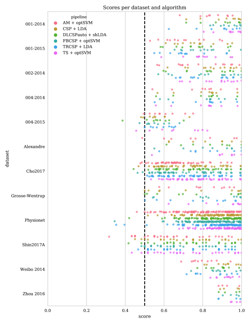
Figure 1: Visualization of all generated scores, across all datasets. The dotted line corresponds to a chance level performance of 0.5

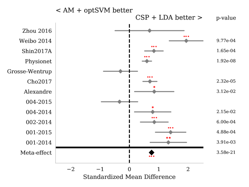
Figure 2: Meta-analysis style plots showing the performance of log variance features (A) and tangent space features (B) both compared against CSP. The effect sizes shown are standardized mean differences, with p-values corresponding to the one-tailed Wilcoxon signed-rank test for the hypothesis given at the top of the plot and 95% interval denoted by the grey bar. Stars correspond to ***=p$<$0.001, **=p$<$0.01, *=p$<$0.05. The meta-effect is shown at the bottom of the plot. While there is a significant amount of variance between datasets–variance that could give contradictory results if these datasets were evaluated in isolation–the overall trend shows that CSP is on average better than channel log-variances and worse than tangent space projection.

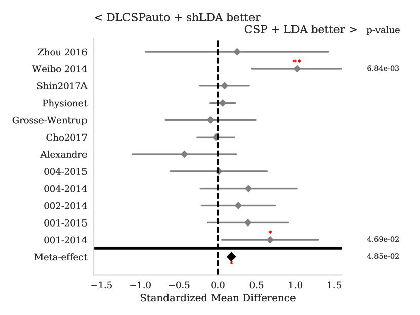
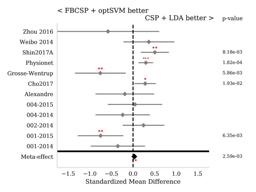
Figure 3: Meta-analysis style plots showing the performance of CSP versus CSP variants: DLCSPauto(A), TRCSP (B), and filter-bank CSP (C). The effect sizes shown are standardized mean differences, with p-values corresponding to the one-tailed Wilcoxon signed-rank test for the hypothesis given at the top of the plot and 95% interval denoted by the grey bar. Stars correspond to ***=p$<$0.001, **=p$<$0.01, *=p$<$0.05. The meta-effect is shown at the bottom of the plot. While there is a significant amount of variance between datasets–variance that could give contradictory results if these datasets were evaluated in isolation–the overall trend shows that CSP out-performs the other algorithms in this setting.

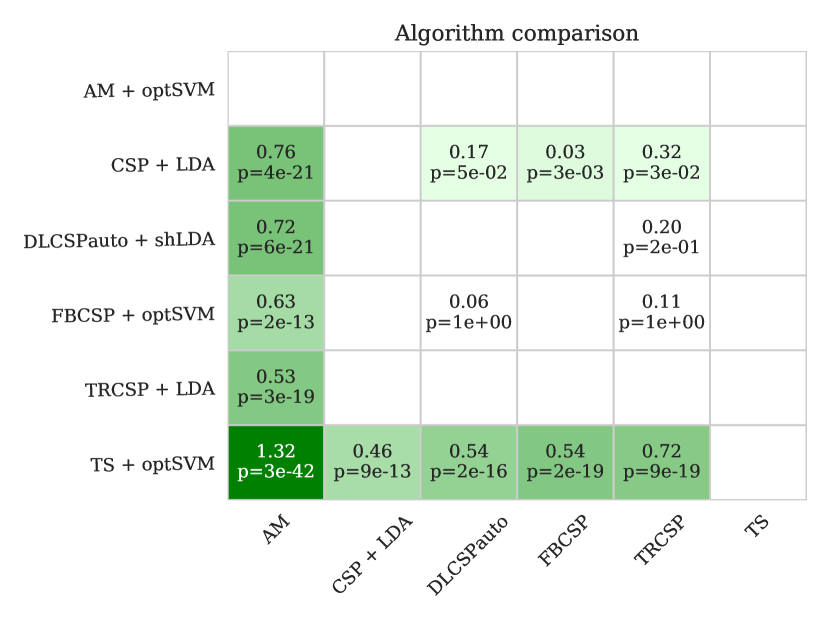
Figure 4: Ranking of algorithms in performance across all datasets with statistics generated as defined in section III. As all p-values are single-sided, in the case that the effect goes in the opposite direction of the hypothesis the values are removed for clarity. The values correspond to the standardized mean difference of the algorithm in the y-axis minus that in the x-axis and the associated p-value

VI Discussion

We present a system for reliably comparing BCI pipelines that is both easily extended to incorporate new datasets and equipped with an automated statistical procedure for determining which pipelines perform best. Furthermore, this system defines a simple interface for submitting and validating new BCI pipelines, which could serve to unify the many methods that exist so far. To test that system, we present results using standard pipelines in contexts that have wide relevance to the BCI community. By looking across multiple, large datasets, it is possible to make statements about how BCIs perform on average, without any sort of expert tuning of the processing chain, and further to see where the major pitfalls still lie.

The results of this analysis suggest that many well-known methods do not reliably out-perform simpler ones, despite the small-scale studies done years ago to validate them. In particular, the world of CSP regularization literature does not appear to have the effect that was originally claimed. Rather, the major difference in BCI classification isn’t actually the algorithm, as of now, but the recording and human paradigm characteristics. The two most clear findings to come out of this are that log variances on the channel level are almost never better than CSP or Riemannian methods, and that the tangent space classification pipeline is the best of the tested models for single-session classification.

In particular in the cases of FBCSP and the regularized approaches presented here, the results presented here are surprising finding as they go against the results reported in the original papers. In the case of FBCSP, we perform similarly to the results shown in [18]. BNCI 2014-001 and 2014-004 are originally from the BCI competitions and were used in the original paper, and our finding is that on these datasets FBCSP indeed out-performed regular CSP. In the case of the regularized variants DLCSPauto and TRCSP, our results on the BCI competition data do not actually follow the originally reported trend. Some possible for reasons are the following: our use of single-session recordings ignores the initial training and test distinctions given within the competition, and we also used the AUC-ROC instead of the accuracy that was reported in the initial analysis. The full code to replicate these results is available publically, and so we hope we can at least rule out improper coding as a source of error.

Looking at these findings, it is particularly interesting to look at the case of filter-bank CSP versus CSP, as in this analysis the significance goes in both directions depending on the dataset. Since datasets vary in many characteristics, such as channel number, imagery type, and trial time, it is hard to determine what exactly underlies this diverging performance – but it is likely that this is not purely by chance. With increasing numbers of available datasets, however, the answers to such differences become possible. If we have many different situations in which to test algorithms, we can determine what factors contribute to the differences in performance between them. It is also important to emphasize that the results shown here must be taken in context. All results were generated by cross-validation within single recording sessions, which limits the possible non-stationarity. Because of this, regularization is at its least useful – which means that it would be inappropriate to dismiss regularization in the case of CSP out of hand. Rather, this same analysis should be re-run in the case of cross-session classification, a task that is currently infeasible due to the number of multi-session datasets.

VII Conclusion

Meta-analysis is a well-described tool in other scientific fields to attempt to synthesize the effects of many different studies that all bear on the same, or very similar hypotheses. Though its use in BCIs has been hampered by the difficulties involved in gathering the data and algorithms in a single place, the MOABB project has the potential to offer a solution to this problem. The analysis here, though done with over 250 subjects, is still only a fraction of the number of subjects recorded for BCI publications over the years. With more papers that describe more varied setups, the power of this system can only grow, and what this analysis shows most clearly is that the sample size problem in BCIs is bigger than we might have expected. By gathering the data and offering a system for testing algorithms, we hope that this platform in the coming years can help to solve it.

References

- [1] Martın Abadi et al. “Tensorflow: Large-scale machine learning on heterogeneous distributed systems” In arXiv preprint arXiv:1603.04467, 2016 URL: https://www.tensorflow.org/
- [2] Brendan Allison et al. “BCI demographics: How many (and what kinds of) people can use an SSVEP BCI?” In Neural Systems and Rehabilitation Engineering, IEEE Transactions on 18.2 IEEE, 2010, pp. 107–116
- [3] Alexandre Barachant “Commande robuste d’un effecteur par une interface cerveau machine EEG asynchrone” Université de Grenoble, 2012 URL: https://tel.archives-ouvertes.fr/tel-01196752/
- [4] Alexandre Barachant, Stéphane Bonnet, Marco Congedo and Christian Jutten “Classification of covariance matrices using a Riemannian-based kernel for BCI applications” In Neurocomputing 112 Elsevier, 2013, pp. 172–178 DOI: 10.1016/J.NEUCOM.2012.12.039
- [5] B Blankertz et al. “The BCI Competition III: Validating Alternative Approaches to Actual BCI Problems” In IEEE Transactions on Neural Systems and Rehabilitation Engineering 14.2, 2006, pp. 153–159
- [6] B Blankertz, G Dornhege, M Krauledat, K R Müller and G Curio “The non-invasive Berlin Brain-Computer Interface: Fast acquisition of effective performance in untrained subjects” In NeuroImage 37.2, 2007, pp. 539–550
- [7] L Bovino et al. “On the combination of” In Analysis 5.33, 2003, pp. 42–54
- [8] Yilun Chen, Ami Wiesel, Yonina C. Eldar and Alfred O. Hero “Shrinkage Algorithms for MMSE Covariance Estimation” In IEEE Transactions on Signal Processing 58.10, 2010, pp. 5016–5029 DOI: 10.1109/TSP.2010.2053029
- [9] Hohyun Cho, Minkyu Ahn, Sangtae Ahn, Moonyoung Kwon and Sung Chan Jun “EEG datasets for motor imagery brain-computer interface” In GigaScience 6.7, 2017, pp. 1–8 DOI: 10.1093/gigascience/gix034
- [10] Jia Deng et al. “Imagenet: A large-scale hierarchical image database” In Computer Vision and Pattern Recognition, 2009. CVPR 2009. IEEE Conference on, 2009, pp. 248–255
- [11] J. Faller, C. Vidaurre, T. Solis-Escalante, C. Neuper and R. Scherer “Autocalibration and Recurrent Adaptation: Towards a Plug and Play Online ERD-BCI” In IEEE Transactions on Neural Systems and Rehabilitation Engineering 20.3, 2012, pp. 313–319 DOI: 10.1109/TNSRE.2012.2189584
- [12] D. Garrett, D.A. A Peterson, C.W. W Anderson and M.H. H Thaut “Comparison of linear, nonlinear, and feature selection methods for EEG signal classification” In IEEE Transactions on Neural Systems and Rehabilitation Engineering 11.2, 2003, pp. 141–144 DOI: 10.1109/TNSRE.2003.814441
- [13] Ary L Goldberger et al. “PhysioBank, PhysioToolkit, and PhysioNet” In Circulation 101.23, 2000, pp. e215 LP –e220 URL: http://circ.ahajournals.org/content/101/23/e215.abstract
- [14] Alexandre Gramfort et al. “MEG and EEG data analysis with MNE-Python” In Frontiers in Neuroscience 7 Frontiers, 2013, pp. 267 DOI: 10.3389/fnins.2013.00267
- [15] Alexandre Gramfort et al. “MNE software for processing MEG and EEG data” In NeuroImage 86, 2014, pp. 446–460 DOI: 10.1016/j.neuroimage.2013.10.027
- [16] M. Grosse-Wentrup, C. Liefhold, K. Gramann and M. Buss “Beamforming in Noninvasive Brain–Computer Interfaces” In IEEE Transactions on Biomedical Engineering 56.4, 2009, pp. 1209–1219 DOI: 10.1109/TBME.2008.2009768
- [17] Vinay Jayaram, Morteza Alamgir, Yasemin Altun, Bernhard Schölkopf and Moritz Grosse-Wentrup “Transfer Learning in Brain-Computer Interfaces” In Computational Intelligence Magazine, IEEE 11.1 IEEE, 2016, pp. 20–31
- [18] Kai Keng Ang, Zhang Yang Chin, Haihong Zhang and Cuntai Guan “Filter Bank Common Spatial Pattern (FBCSP) in Brain-Computer Interface” In 2008 IEEE International Joint Conference on Neural Networks (IEEE World Congress on Computational Intelligence) IEEE, 2008, pp. 2390–2397 DOI: 10.1109/IJCNN.2008.4634130
- [19] Zoltan J Koles, Michael S Lazar and Steven Z Zhou “Spatial patterns underlying population differences in the background EEG” In Brain Topography 2.4 Springer, 1990, pp. 275–284
- [20] R. Leeb et al. “Brain-Computer Communication: Motivation, Aim, and Impact of Exploring a Virtual Apartment” In IEEE Transactions on Neural Systems and Rehabilitation Engineering 15.4, 2007, pp. 473–482 DOI: 10.1109/TNSRE.2007.906956
- [21] Miguel Angel Lopez-Gordo, Daniel Sanchez-Morillo and F Pelayo Valle “Dry EEG electrodes” In Sensors 14.7 Multidisciplinary Digital Publishing Institute, 2014, pp. 12847–12870
- [22] F Lotte and C Guan “Regularizing common spatial patterns to improve BCI designs: unified theory and new algorithms” In IEEE Transactions on Biomedical Engineering 58.2 Institute of ElectricalElectronics Engineers, Inc., 345 E. 47 th St. NY NY 10017-2394 USA, 2011, pp. 355–362
- [23] Adam Paszke et al. “Automatic differentiation in PyTorch”, 2017 URL: https://openreview.net/forum?id=BJJsrmfCZ
- [24] Fabian Pedregosa et al. “Scikit-learn: Machine Learning in Python” In Journal of Machine Learning Research 12.Oct, 2011, pp. 2825–2830 URL: http://jmlr.csail.mit.edu/papers/v12/pedregosa11a.html
- [25] G. Schalk, D.J. McFarland, T. Hinterberger, N. Birbaumer and J.R. Wolpaw “BCI2000: A General-Purpose Brain-Computer Interface (BCI) System” In IEEE Transactions on Biomedical Engineering 51.6, 2004, pp. 1034–1043 DOI: 10.1109/TBME.2004.827072
- [26] Reinhold Scherer et al. “Individually Adapted Imagery Improves Brain-Computer Interface Performance in End-Users with Disability” In PLOS ONE 10.5 Public Library of Science, 2015, pp. e0123727 DOI: 10.1371/journal.pone.0123727
- [27] A Schloegl “Results of the BCI Competition 2005 for data set IIIa and IIIb”, 2005
- [28] A Searle and L Kirkup “A direct comparison of wet, dry and insulating bioelectric recording electrodes” In Physiological measurement 21.2 IOP Publishing, 2000, pp. 271
- [29] Jaeyoung Shin et al. “Open Access Dataset for EEG+NIRS Single-Trial Classification” In IEEE Transactions on Neural Systems and Rehabilitation Engineering 25.10, 2017, pp. 1735–1745 DOI: 10.1109/TNSRE.2016.2628057
- [30] David Steyrl, Reinhold Scherer, Josef Faller and Gernot R. Müller-Putz “Random forests in non-invasive sensorimotor rhythm brain-computer interfaces: a practical and convenient non-linear classifier” In Biomedical Engineering 61.1 De Gruyter, 2016, pp. 77–86 DOI: 10.1515/bmt-2014-0117
- [31] Samuel A. Stouffer, Edward A. Suchman, Leland C. Devinney, Shirley A. Star and Robin M. Williams Jr. “The American soldier: Adjustment during army life. (Studies in social psychology in World War II)” Oxford, England: Princeton University Press, 1949 URL: http://psycnet.apa.org/record/1950-00790-000
- [32] Michael Tangermann et al. “Review of the BCI Competition IV” In Frontiers in Neuroscience 6 Frontiers, 2012, pp. 55 DOI: 10.3389/fnins.2012.00055
- [33] Weibo Yi et al. “Evaluation of EEG Oscillatory Patterns and Cognitive Process during Simple and Compound Limb Motor Imagery” In PLoS ONE 9.12 Public Library of Science, 2014, pp. e114853 DOI: 10.1371/journal.pone.0114853
- [34] Han Yuan and Bin He “Brain-computer interfaces using sensorimotor rhythms: current state and future perspectives.” In IEEE Transactions on Biomedical Engineering 61.5 NIH Public Access, 2014, pp. 1425–35 DOI: 10.1109/TBME.2014.2312397
- [35] Bangyan Zhou, Xiaopei Wu, Zhao Lv, Lei Zhang and Xiaojin Guo “A Fully Automated Trial Selection Method for Optimization of Motor Imagery Based Brain-Computer Interface” In PLOS ONE 11.9 Public Library of Science, 2016, pp. e0162657 DOI: 10.1371/journal.pone.0162657