Semi-exact solutions of the Razavy potential

Abstract

In this work we study the quantum system with the symmetric Razavy potential and show how to find its exact solutions. We find that the solutions are given by the confluent Heun functions. The eigenvalues have to be calculated numerically. The properties of the wave functions depending on $m$ are illustrated graphically for a given potential parameter $\xi$. We find that the even and odd wave functions with definite parity are changed to odd and even wave functions when the potential parameter $m$ increases. This arises from the fact that the parity, which is a defined symmetry for very small $m$, is completely violated for large $m$. We also notice that the energy levels $\epsilon_{i}$ decrease with the increasing potential parameter $m$.

I Introduction

It is well known that the exact solutions of quantum systems play an important role since the early foundation of the quantum mechanics. Generally speaking, two typical examples are studied for the hydrogen atom and harmonic oscillator in classical quantum mechanics textbooks [1, 2]. Up to now, there are a few main methods to solve the quantum soluble systems. The first is called the functional analysis method. That is to say, one solves the second-order differential equation and obtains their solutions [3], which are expressed by some well-known special functions. The second is called the algebraic method, which is realized by studying the Hamiltonian of quantum system. This method is also related with supersymmetric quantum mechanics (SUSYQM)[4], further closely with the factorization method [5]. The third is called as the exact quantization rule method [6], from which we proposed proper quantization rule [7], which shows more beauty and symmetry than exact quantization rule. It should be recognized that almost all soluble potentials mentioned above belong to single well potentials. The double well potentials have not been studied well due to their complications [8-17], in which many authors have been searching the solutions of the double-well potentials for a long history. This is because the double well potentials could be used in the quantum theory of molecules to describe the motion of the particle in the presence of two centers of force, the heterostructures, Bose-Einstein condensates and superconducting circuits, etc.

Almost forty years ago, Razavy proposed a bistable potential [18]

$$V(x)=\frac{\hbar^{2}\beta^{2}}{2\mu}\left[\frac{1}{8}\xi^{2}\cosh(4\beta x)-(m+1)\xi\cosh(2\beta x)-\frac{1}{8}\xi^{2}\right],$$ (1)

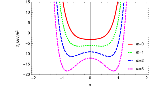
Figure 1: (Color online) A plot of potential as function of the variables $x$ and $m$.

which depends on three potential parameters $\beta$, $\xi$ and a positive integer $m$. In Fig. 1 we plot it as the function of the variables $x$ with various $m$, in which we take $\beta=1$ and $\xi=3$. Choose atomic units $\hbar=\mu=1$ and also take $\mathcal{V}(x)=2V(x)$. Using series expansion around the origin, we have

$$\mathcal{V}(x)=(-m\xi-\xi)+x^{2}\left(-2m\xi+\xi^{2}-2\xi\right)+\frac{2}{3}x^{4}\left(-m\xi+2\xi^{2}-\xi\right)+\frac{4}{45}x^{6}\left(-m\xi+8\xi^{2}-\xi\right)+O\left(x^{7}\right),$$ (2)

which shows that $\mathcal{V}(x)$ is symmetric to variable $x$. We find that the minimum value of the potential $\mathcal{V}_{\rm min}(x)=-(m+1)^{2}-\xi^{2}/4$ at two minimum values $x=\pm\frac{1}{2}\cosh^{-1}[2(m+1)/\xi]$. For a given value $\xi=3$, we find that the potential has a flat bottom for $n=0$, but for $n>1$ it takes the form of a double well. Razavy presented the so-called exact solutions by using the ”polynomial method” [18]. After studying it carefully, we find that the solutions cannot be given exactly due to the complicated three-term recurrence relation. The method presented there [18] is more like the Bethe Ansatz method as summarized in our recent book [19]. That is, the solutions cannot be expressed as one of special functions because of three-term recurrence relations. In order to obtain some so-called exact solutions, the author has to take some constraints on the coefficients in the recurrence relations as shown in Ref. [18]. Inspired by recent study of the hyperbolic type potential well [20-28], in which we have found that their solutions can be exactly expressed by the confluent Heun functions [23], in this work we attempt to study the solutions of the Razavy potential. We shall find that the solutions can be written as the confluent Heun functions but their energy levels have to be calculated numerically since the energy term is involved within the parameter $\eta$ of the confluent Heun functions $H_{c}(\alpha,\beta,\gamma,\delta,\eta,z)$. This constraints us to use the traditional Bathe ansatz method to get the energy levels. Even though the Heun functions have been studied well, its main topics are focused in the mathematical area. Only recent connections with the physical problems have been discovered, in particular the quantum systems for those hyperbolic type potential have been studied [20-28]. The terminology ”semi-exact” solutions used in Ref. [21] arises from the fact that the wave functions can be obtained analytically, but the eigenvalues cannot be written out explicitly.

This paper is organized as follows. In Sect. 2, we present the solutions of the Schrödinger equation with the Razavy potential. It should be recognized that the Razavy potential is single or double well depends on the potential parameter $m$. In Sect. 3 some fundamental properties of the solutions are studied. The energy levels for different $m$ are calculated numerically. Some concluding remarks are given in Sect. 4.

II Semi-exact solutions

Let us consider the one-dimensional Schrödinger equation,

$$-\frac{\hbar^{2}}{2\mu}\frac{d^{2}}{dx^{2}}\psi(x)+V(x)\psi(x)=E\psi(x).$$ (3)

Substituting potential (1) into (3), we have

$$\frac{d^{2}}{dx^{2}}\psi(x)+\left\{\varepsilon-\left[\frac{1}{8}\xi^{2}\cosh(4x)-(m+1)\xi\cosh(2x)-\frac{1}{8}\xi^{2}\right]\right\}\psi(x)=0,~{}~{}~{}~{}\epsilon=2E.$$ (4)

Take the wave functions of the form

$$\psi(x)=e^{\frac{\xi\cosh^{2}(x)}{2}}y(x).$$ (5)

Substituting this into Eq. (4) allows us to obtain

$$y^{\prime\prime}(x)+\xi\sinh(2x)y^{\prime}(x)+[(m+2)\xi\cosh(2x)+\epsilon]y(x)=0.$$ (6)

Take a new variable $z=\cosh^{2}(x)$. The above equation becomes

$$4(z-1)zy^{\prime\prime}(z)+[4z(\xi(z-1)+1)-2]y^{\prime}(z)+((m+2)\xi(2z-1)+\epsilon)y(z)=0.$$ (7)

which can be re-arranged as

$$y^{\prime\prime}(z)+\left[\xi+\frac{1}{2}\left(\frac{1}{z}+\frac{1}{z-1}\right)\right]y^{\prime}(z)+\frac{(m+2)\xi(2z-1)+\epsilon}{4(z-1)z}y(z)=0.$$ (8)

When comparing this with the confluent Heun differential equation in the simplest uniform form [13]

$$\frac{d^{2}H(z)}{dz^{2}}+\left(\alpha+\frac{1+\beta}{z}+\frac{1+\gamma}{z-1}\right)\frac{dH(z)}{dz}+\left(\frac{\mu}{z}+\frac{\nu}{z-1}\right)H(z)=0,$$ (9)

we find the solution to (8) is given by the acceptable confluent Heun function $H_{c}(\alpha,\beta,\gamma,\delta,\eta;z)$ with

$$\alpha=\xi,~{}~{}~{}\beta=-\frac{1}{2},~{}~{}~{}\gamma=-\frac{1}{2},~{}~{}~{}\mu=\frac{\xi(m+2)-\varepsilon}{4},~{}~{}~{}\nu=\frac{\xi(m+2)+\varepsilon}{4},$$ (10)

from which we are able to calculate the parameters $\delta$ and $\eta$ involved in $H_{c}(\alpha,\beta,\gamma,\delta,\eta;z)$ as

$$\delta=\mu+\nu-\frac{1}{2}\alpha(\beta+\gamma+2)=\frac{1}{2}(m+1)\xi,~{}~{}~{}~{}\eta=\frac{1}{2}\alpha(\beta+1)-\mu-\frac{1}{2}(\beta+\gamma+\beta\gamma)=\frac{1}{8}[-2(m+1)\xi+2\epsilon+3].$$ (11)

It is found that the parameter $\eta$ related to energy levels is involved in the confluent Heun function. The wave function given by this function seems to be analytical, but the key issue is how to first get the energy levels. Otherwise, the solution becomes unsolvable. Generally, the confluent Heun function can be expressed as a series expansions

$$H_{C}(\alpha,\beta,\gamma,\delta,\eta,z)=\sum\limits_{n=0}^{\infty}v_{n}(\alpha,\beta,\gamma,\delta,\eta,\xi)z^{n},~{}~{}~{}~{}|z|<1.$$ (12)

The coefficients $v_{n}$ are given by a three-term recurrence relation

$$A_{n}v_{n}-B_{n}v_{n-1}-C_{n}v_{n-2}=0,~{}~{}~{}v_{-1}=0,~{}~{}~{}v_{0}=1,$$ (13)

with

$$\begin{array}[]{l}A_{n}=1+\displaystyle\frac{\beta}{n},\\[5.69054pt] B_{n}=1+\displaystyle\frac{1}{n}(\beta+\gamma-\alpha-1)+\frac{1}{n^{2}}\left\{\eta-\frac{1}{2}(\beta+\gamma-\alpha)-\frac{\alpha\beta}{2}+\frac{\beta\gamma}{2}\right\},\\[5.69054pt] C_{n}=\displaystyle\frac{\alpha}{n^{2}}\left(\frac{\delta}{\alpha}+\frac{\beta+\gamma}{2}+n-1\right).\end{array}$$ (14)

To make the confluent Heun functions reduce to polynomials, two termination conditions have to be satisfied [13, 14]

$$\mu+\nu+N\alpha=0,~{}~{}~{}~{}\Delta_{N+1}(\mu)=0,$$ (15)

where

$$\left|\begin{array}[]{ccccccc}\mu-p_{1}&(1+\beta)&0&\ldots&0&0&0\\ N\alpha&\mu-p_{2}+\alpha&2(2+\beta)&\ldots&0&0&0\\ 0&(N-1)\alpha&\mu-p_{3}+2\alpha&\ldots&0&0&0\\ \vdots&\vdots&\vdots&\ddots&\vdots&\vdots&\vdots\\ 0&0&0&\ldots&\mu-p_{N-1}+(N-2)\alpha&(N-1)(N-1+\beta)&0\\ 0&0&0&\ldots&2\alpha&\mu-p_{N}+(N-1)\alpha&N(N+\beta)\\ 0&0&0&\ldots&0&\alpha&\mu-p_{N+1}+N{\alpha}\end{array}\right|=0$$ (16)

with

$$p_{N}=(N-1)(N+\beta+\gamma).$$ (17)

For present problem, it is not difficult to see that the first condition is violated. That is, $\mu+\nu+\alpha=0$ when $N=1$. From this we have $m=-4$. This is contrary to the fact $m$ is a positive integer. Therefore we cannot use this method to obtain the eigenvalues. On the other hand, we know that $z\in[1,\infty)$. Thus, the series expansion method is invalid. This is unlike previous study [22, 24], in which the quasi-exact wave functions and eigenvalues can be obtained by studying those two constraints. The present case is similar to our previous study [20, 21], in which some constraint is violated. We have to choose other approach to study the eigenvalues as used in [20,21].

III Fundamental properties

In this section we are going to study some basic properties of the wave functions as shown in Figs. 2-4. We first consider the positive integer $m$. Since the energy spectrum cannot be given explicitly we have to solve the second order differential equation (4) numerically. We denote the energy levels as $\epsilon_{i}(i\in[1,6])$ in Table 1. We find that the energy levels $\epsilon_{i}$ decrease with the increasing $m$. Originally, we wanted to calculate the energy levels numerically by using powerful MAPLE, which includes some special functions such as the confluent Heun function that cannot be found in MATHEMATICA. As we know, the wave function is given by $\psi(z)=\exp(z\xi/2)H_{c}(\alpha,\beta,\gamma,\delta,\eta,z)$. Generally speaking, the wave function requires $\psi(z)\to 0$ when $z\to\infty$, i. e. $x\to\infty$. Unfortunately, the present study is unlike our previous study [20,21], in which $z\to 1$ when $x$ goes to infinity. The energy spectra can be calculated by series expansions through taking $z\to 1$. On the other hand, the wave functions have a definite parity, e.g for $m=0$ some wave functions are symmetric. It is found that such properties are violated when the potential parameter $m$ becomes larger as shown in Fig. 4. That is, the wave functions for $m=12$ is nonsymmetric. In addition, on the contrary to the case discussed by Razavy [18], in which he supposed the $m$ is taken as positive integers, we are going to show what happens to the negative $m$ case. We display the graphics in Figs. 5 and 6 for this case. We find that the wave functions are shrunk towards the origin. This makes the amplitude of the wave function is increasing.

IV Conclusions

In this work we have studied the quantum system with the Razavy potential, which is symmetric with respect to the variable $x$, and shown how its exact solutions are found by transforming the original differential equation into a confluent type Heun differential equation. It is found that the solutions can be expressed by the confluent Heun functions $Hc(\alpha,\beta,\gamma,\delta,\eta)$, in which the energy levels are involved inside the parameter $\eta$. This makes us to calculate the eigenvalues numerically. The properties of the wave functions depending on $m$ are illustrated graphically for a given potential parameter $\xi$. We have found that the even and odd wave functions with definite parity are changed to odd and even wave functions when the potential parameter $m$ increases. This arises from the fact that the parity, which is a defined symmetry for very small $m$, is completely violated for large $m$. We have also noticed that the energy levels $\epsilon_{i}$ decrease with the increasing potential parameter $m$.

Competing Interests
The authors declare that there is no conflict of interests regarding the publication of this paper.

Acknowledgments: This work is supported by project 20180677-SIP-IPN, COFAA-IPN, Mexico and partially by the CONACYT project under grant No. 288856-CB-2016 and partially by NSFC with Grant No. 11465006.

Table 1: Energy levels of the Schrödinger equation with potential (1)

$\nu$	$\epsilon_{1}$	$\epsilon_{2}$	$\epsilon_{3}$	$\epsilon_{4}$	$\epsilon_{5}$	$\epsilon_{6}$
$m=-6$	21.6608	35.7557	51.3448	68.3341	86.6500	106.233
$m=-5$	18.1891	31.3844	46.1503	62.3746	79.9715	98.8740
$m=-4$	14.6806	26.9167	40.8214	56.2549	73.1150	91.3249
$m=-3$	11.1259	22.3314	35.3346	49.9525	66.0599	83.5680
$m=-2$	7.51110	17.5996	29.6610	43.4412	58.7838	75.5860
$m=-1$	3.81463	12.6800	23.7644	36.6914	51.2639	67.3635
$m=0$	0.00007	7.51170	17.6027	29.6729	43.4799	58.8919
$m=1$	-3.99968	2.00200	11.1343	22.3606	35.4208	50.1750
$m=2$	-8.32288	-3.99300	4.34771	14.7494	27.0959	41.2385
$m=3$	-13.2815	-10.6927	-2.64788	6.87526	18.5501	32.1389
$m=4$	-19.5196	-9.46859	-1.17161	9.87916	22.9677	38.0537
$m=5$	-27.7547	-15.7094	-9.29612	1.24110	13.8439	28.5940
$m=6$	-38.0314	-21.6913	-17.5131	-7.12621	4.89289	19.3065
$m=7$	-49.9928	-28.2027	-25.9897	-14.8827	-3.78434	10.2625
$m=8$	-63.3335	-35.8866	-21.7455	-12.1464	1.51447	17.5661
$m=9$	-77.8339	-44.5255	-27.8571	-20.2355	-6.89162	8.76577
$m=10$	-93.3024	-54.9017	-33.6970	-28.1690	-14.8944	0.229704
$m=11$	-109.592	-65.743	-39.7373	-36.1005	-22.4007	-8.04337
$m=12$	-126.580	-77.2416	-46.3335	-29.3139	-16.0647	1.06475

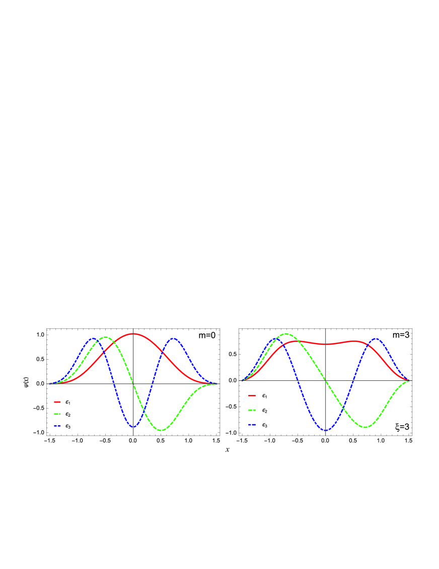
Figure 2: (Color online) The characteristics of the potential ${\cal V}(z)$ as a function of the position $z$. We take $m=0,1$ and $\xi=3$.

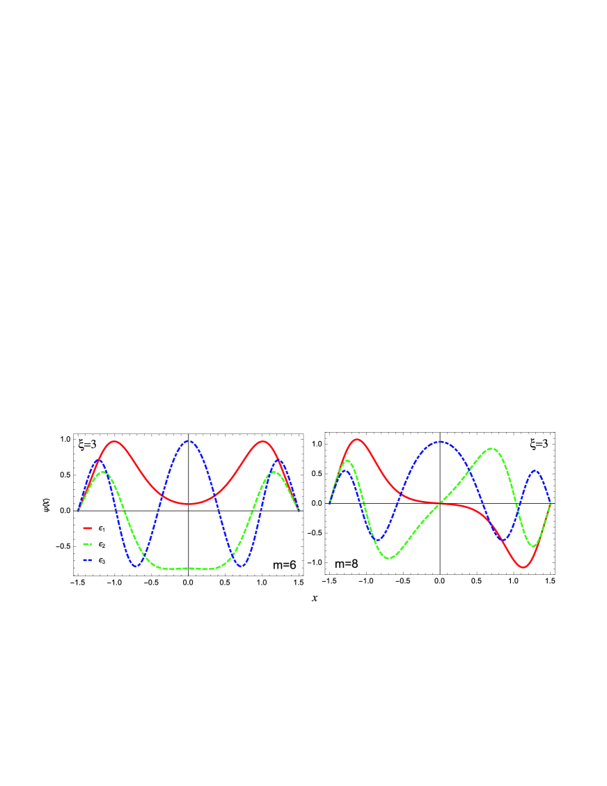
Figure 3: (Color online) The characteristics of the potential ${\cal V}(z)$ as a function of the position $z$. We take $m=6,8$ and $\xi=3$.

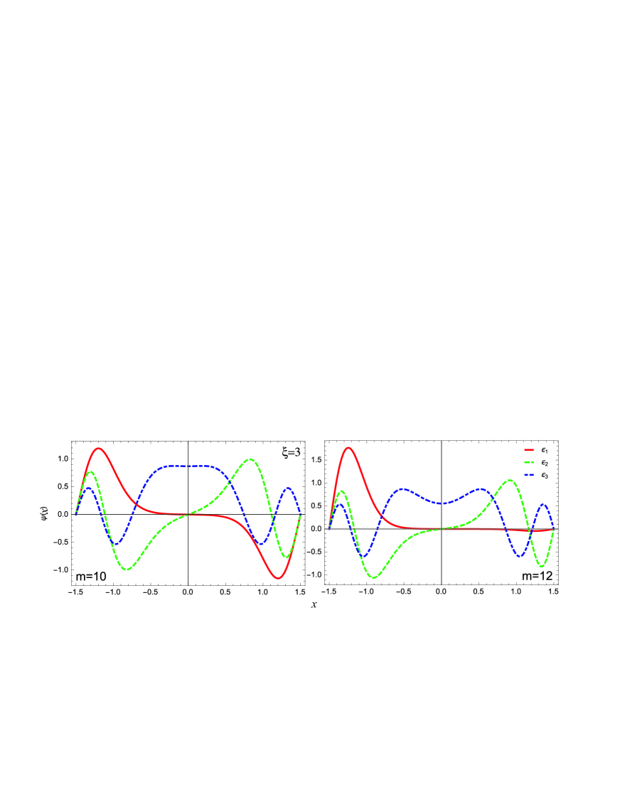
(3)

Figure 4: (Color online)Same as above case but $m=10,12$.

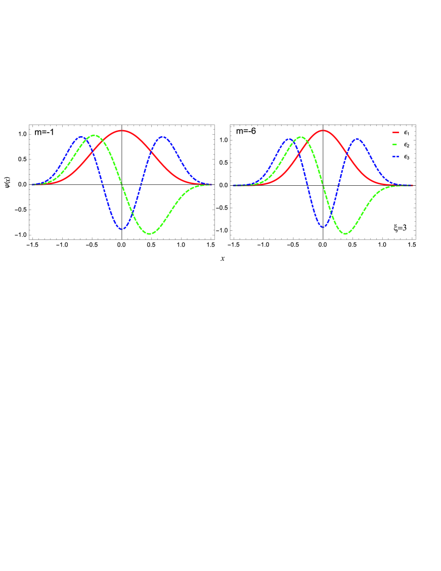
Figure 5: (Color online) The characteristics of the potential ${\cal V}(z)$ as a function of the position $z$. We take $m=-1,-6$ and $\xi=3$.

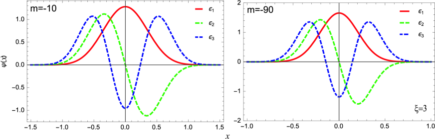
Figure 6: (Color online)Same as above case but $m=-10,-90$.

References

- (1) L. I. Schiff, Quantum Mechanics 3rd ed. New York, McGraw-Hill Book Co. , 1955.
- (2) L. D. Landau and E. M. Lifshitz, Quantum Mechanics (Non-Relativistic Theory) 3rd ed. Pergamon, New York, 1977.
- (3) D. ter Haar, Problems in Quantum Mechanics 3rd Ed. , Pion Ltd, London, 1975.
- (4) F. Cooper, A. Khare and U. Sukhatme, Phys. Rep. 251, 267 (1995).
- (5) S. H. Dong, Factorization Method in Quantum Mechanics, Springer, Kluwer Academic Publisher, 2007.
- (6) Z. Q. Ma and B. W. Xu, Europhys. Lett. 69, 685 (2005).
- (7) W. C. Qiang and S. H. Dong, EPL 89, 10003 (2010).
- (8) N. Rosen, P.M. Morse, Phys. Rev. 42, 210(1932).
- (9) M. F. Manning, J. Chem. Phys. 3, 136 (1935).
- (10) M. Baradaran and H. Panahi, Advances in High Energy Physics Volume 2017, Article ID 2181532 (2017).
- (11) H. Konwent, Phys. Lett. A 118, 467 (1986).
- (12) H. Konwent, P. Machnikowski, A. Radosz, J. Phys. A: Math. Gen. 28, 3757(1995).
- (13) Qiong-Tao Xie, J. Phys. A: Math. Theor. 45, 175302 (2012).
- (14) Bei-Hua Chen, Yan Wu, Qiong-Tao Xie, J. Phys. A: Math. Theor. 46, 035301 (2013).
- (15) R.R. Hartmann, J.Math.Phys. 55, 012105 (2014).
- (16) A. E. Sitniksky, Chem. Phys. Lett. 676, 169 (2017).
- (17) Dai-Nam Le, Ngoc-Tram D. Hoang, and Van-Hoang Le, J. Math. Phys. 59, 032101(2018).
- (18) M. Razavy, Am. J. Phys. 48(4), 285 (1980).
- (19) S. H. Dong, Wave Equations in Higher Dimensions, Springer, 2011.
- (20) S. Dong, Q. Fang, B. J. Falaye, G. H. Sun, C. Yáñez-Márquez, S. H. Dong, Mod. Phys. Lett. A 31(04), 1650017 (2016)
- (21) S. Dong, G. H. Sun, B. J. Falaye and S. H. Dong, The European Physical Journal Plus 131(5), 176 (2016).
- (22) G. H. Sun, S. H. Dong, K. D. Launey, T. Dytrych, J. P. Draayer, Int. J. Quan. Chem. 115(14), 891 (2015).
- (23) A. Ronveaux (ed) Heun’s Differential Equations, Oxford: Oxford University Press, 1995.
- (24) C. A. Downing, J. Math. Phys. 54, 072101 (2013).
- (25) P. P. Fiziev, J. Phys. A: Math. Theor. 43, 035203 (2010).
- (26) R. Hartmann, M. E. Portnoi, Phys. Rev. A 89, 012101 (2014).
- (27) D. Agboola, J. Math. Phys. 55, 052102 (2014).
- (28) F. K. Wen, Z. Y. Yang, C. Liu, W. L. Yang and Y. Z. Zhang, Commun. Theor. Phys. 61, 153 (2014).