Tensor completion for Color Images and Videos

Abstract

Tensor completion recovers missing entries of multiway data. The missing of entries could often be caused during the data acquisition and transformation. In this paper, we provide an overview of recent development in low rank tensor completion for estimating the missing components of visual data, e. g. , color images and videos. First, we categorize these methods into two groups based on the different optimization models. One optimizes factors of tensor decompositions with predefined tensor rank. The other iteratively updates the estimated tensor via minimizing the tensor rank. Besides, we summarize the corresponding algorithms to solve those optimization problems in details. Numerical experiments are given to demonstrate the performance comparison when different methods are applied to color image and video processing.

1 Introduction

Multidimensional data is becoming important for dealing with the science and engineering problems. In these fields, the size of data is increasing. Tensor, which is a generation of matrix, provides a natural way to represent multidimensional data. For example, a color image is a third-order tensor, which has two indexes in the spatial space and one index in the color. Besides, a color video is a forth-order tensor with an additional index in the time variable. Employing tensor analysis to process multidimensional data, such as in signal and image processing 1 ; 2 ; 3 ; 4 ; 5 ; 6 ; 7 ; 8 ; 9 , Quantum Chemistry 10 ; 11 ; 12 , computer vision  13 ; 14 ; 15 and data mining 16 ; 17 ; 18 , has aroused more attention in recent years. In most case, some entries of the acquired multidimensional data are missed. Hence, a well-performed recovery technology should be proposed.

Completion tries to recover the missing data from its observed data according to some prior information. With the success of low rank matrix completion 19 ; 20 ; 21 ; 22 ; 23 ; 24 ; 25 ; 26 ; 27 ; 28 , low rank tensor completion is an extension to process the multi-dimensional data. Owing to the different decomposition formats, a series of tensor completion methods are proposed. In order to know about the development of the tensor completion in processing color images and videos, we provide a review to cover the recently methods in this field. The related work in 29 summarizes the tensor completion algorithms in big data analytics. Compared with it, the difference are as follows: (1). Our survey for tensor completion mainly focus on the field in images and videos processing and we do some experiments using the images to test the algorithms; (2). Compared with CP decomposition and Tucker decomposition adopted in previous work, we introduce additional decomposition methods, such as t-SVD, tensor train decomposition and tensor ring decomposition. (3). We mainly divide the tensor completion into two groups. For each group, based on different tensor decomposition methods, we offer several optimization models and algorithms.

The rest of this paper is organized as follows. Section 2 introduces some notations and preliminaries for tensor decomposition. In Section 3, the matrix completion is reviewed. The detailed overview of tensor completion is presented in Section 4. Section 5 provides some experiments for tensor completion using different tensor decomposition formats. The conclusion are concluded in Sec. 6. Finally, the discussion and future work are presented in Sec. 7.

2 Notaions and Preliminaries

A scalar, a vector, a matrix, and a tensor are written as $a$, $\mathbf{a}$, $\mathbf{A}$, and $\mathcal{A}$, respectively. $a^{*}$ denotes the conjugate of $a$. The matrix nuclear norm of $\mathbf{A}$ is denoted as $\lVert{\bf A}\rVert_{*}=\sum_{n=1}^{N}\sigma_{n}(\bf A)$, where $\sigma_{n}(\bf A)$ is the singular value of matrix A. For a $N$-order tensor $\mathcal{A}\in\mathbb{R}^{I_{1}\times\cdots\times I_{N}}$, the multi-index is defined as $\overline{i_{1}i_{2}\cdots i_{N}}=i_{1}+(i_{2}-1)I_{1}+(i_{3}-1)I_{1}I_{2}+\cdots+(i_{N}-1)I_{1}\cdots I_{N-1}$ for $i_{n}=1,2,\cdots,I_{n}$, $n=1,2,\cdots,N$.The vectorization of tensor $\mathcal{A}$ is denoted as $vec({\mathcal{A}})$. The $``\operatorname{reshape}"$ is a reshaping operation from a matrix or a vector to a tensor, e.g., we can obtain a 3rd=order tensor $\mathcal{X}\in\mathbb{R}^{I_{1}\times I_{2}\times I_{3}}$ by the operating $\operatorname{reshape}(\mathbf{X},I_{1},I_{2},I_{3})$ from a matrix $\mathbf{X}\in\mathbb{R}^{I_{1}I_{2}\times I_{3}}$ or $\operatorname{reshape}(\mathbf{x},I_{1},I_{2},I_{3})$ from a vector $\mathbf{x}\in\mathbb{R}^{I_{1}I_{2}I_{3}}$. The most common typed of tensor operations can be see Table 1.

Table 1: Main tensor/matrix products

$\textbf{A}_{<k>}\in\mathbb{R}^{I_{1}\cdots I_{k}\times I_{k+1}\cdots I_{N}}$	k-unfolding of $\mathcal{A}$
$\textbf{A}_{[k]}\in\mathbb{R}^{I_{k}\times I_{1}\cdots I_{k-1}I_{k+1}\cdots I_{N}}$	mode-k unfolding $\mathcal{A}$
$c=<\mathcal{A},\mathcal{B}>$	inner product of $\mathcal{A}$ and $\mathcal{B}$ with the same size
$\mathcal{C}=\mathcal{A}\otimes\mathcal{B}\in\mathbb{R}^{I_{1}J_{1}\times\cdots\times I_{N}J_{N}}$	Kronecker product of $\mathcal{A}\in\mathbb{R}^{I_{1}\times\cdots\times I_{N}}$ and $\mathcal{B}\in\mathbb{R}^{J_{1}\times\cdots\times J_{N}}$
$\mathcal{C}=\mathcal{A}\circ\mathcal{B}\in\mathbb{R}^{I_{1}\times\cdots\times I_{N}\times J_{1}\times\cdots\times J_{N}}$	tensor or outer product of $\mathcal{A}\in\mathbb{R}^{I_{1}\times\cdots\times I_{N}}$
	and $\mathcal{B}\in\mathbb{R}^{J_{1}\times\cdots\times J_{M}}$
$\mathcal{C}=\mathcal{A}\times_{n}\mathbf{B}\in\mathbb{R}^{I_{1}\times\cdots\times I_{n-1}\times J\times I_{n+1}\cdots\times I_{N}}$	mode-n product of $\mathcal{A}\in\mathbb{R}^{I_{1}\times\cdots\times I_{N}}$ and a matrix $\mathbf{B}\in\mathbb{R}^{J\times I_{n}}$
$\mathcal{C}=<\mathcal{A},\mathcal{B}>_{L}\in\mathbb{R}^{I_{1}\times\cdots\times I_{N}\times Q_{1}\times\cdots\times Q_{M}}$	contracted product of $\mathcal{A}\in\mathbb{R}^{I_{1}\times\cdots\times I_{N}\times P_{1}\times\cdots\times P_{L}}$
	and $\mathcal{B}\in\mathbb{R}^{P_{1}\times\cdots\times P_{L}\times Q_{1}\times\cdots\times Q_{M}}$
$\mathcal{U}=\mathcal{U}_{1}\mathcal{U}_{2}\cdots\mathcal{U}_{N}\in\mathbb{R}^{S_{1}\times(I_{1}\cdots I_{N})\times S_{N+1}}$	connection product of 3-order tensors $\mathcal{U}_{n}\in\mathbb{R}^{S_{n}\times I_{n}\times S_{n+1}}$

Definition 1

(k-unfolding 30 ) For an $N$-order tensor $\mathcal{A}\in\mathbb{R}^{I_{1}\times\cdots\times I_{N}}$ whose k-unfolding is defined as a matrix

$$\textbf{A}_{<k>}\in\mathbb{R}^{I_{1}\cdots I_{k}\times I_{k+1}\cdots I_{N}}$$

with entries

$$\textbf{A}_{<k>}(\overline{i_{1}i_{2}\cdots i_{k}},\overline{i_{k+1}\cdots i_{N}})=a_{i_{1}i_{2}\cdots i_{N}},$$

where $a_{i_{1}i_{2}\cdots i_{N}}$ is the $i_{1}i_{2}\cdots i_{N}$-th element of $\mathcal{A}$.

Definition 2

(Mode-k unfolding 30 ) For an $N$-order tensor $\mathcal{A}\in\mathbb{R}^{I_{1}\times\cdots\times I_{N}}$, its mode-k unfolding is defined as a matrix

$$\textbf{A}_{[k]}\in\mathbb{R}^{I_{k}\times I_{1}\cdots I_{k-1}I_{k+1}\cdots I_{N}}$$

with entries

$$\textbf{A}_{[k]}(i_{k},\overline{i_{1}\cdots i_{k-1}i_{k+1}\cdots i_{N}})=a_{i_{1}i_{2}\cdots i_{N}},$$

where $a_{i_{1}i_{2}\cdots i_{N}}$ is the $i_{1}i_{2}\cdots i_{N}$-th element of $\mathcal{A}$.

Definition 3

(Tensor inner product) For two tensors $\mathcal{A}$ and $\mathcal{B}$ with the same size, their inner product is defined as $<\mathcal{A},\mathcal{B}>=<\operatorname{vec}(\mathcal{A}),\operatorname{vec}(\mathcal{B})>$, where $\operatorname{vec}(\mathcal{A})=\operatorname{vec}({\bf{A}}_{<1>})$.

Definition 4

(Tensor Frobenius norm) The Frobenius norm of a tensor is defined as $\|\mathcal{A}\|_{\operatorname{F}}^{2}=<\operatorname{vec}(\mathcal{A}),\operatorname{vec}(\mathcal{A})>$.

Definition 5

(Tensor Kronecker product) For multiway arrays $\mathcal{A}\in\mathbb{R}^{I_{1}\times\cdots\times I_{N}}$ and $\mathcal{B}\in\mathbb{R}^{J_{1}\times\cdots\times J_{N}}$, the Kronecker product can be denoted as $\mathcal{C}=\mathcal{A}\otimes\mathcal{B}\in\mathbb{R}^{I_{1}J_{1}\times\cdots\times I_{N}J_{N}}$ with entries $c_{i_{1}j_{1},\dots,i_{N}j_{N}=a_{i_{1},\dots,i_{N}}b_{j_{1},\dots,j_{N}}}$, where $i_{n}j_{n}=j_{n}+(i_{n}-1)J_{n}$.

Definition 6

(Tensor or outer product) For two tensors $\mathcal{A}\in\mathbb{R}^{I_{1}\times\cdots\times I_{N}}$ and $\mathcal{B}\in\mathbb{R}^{J_{1}\times\cdots\times J_{M}}$, the tensor or outer product can be defined as $\mathcal{C}=\mathcal{A}\circ\mathcal{B}\in\mathbb{R}^{I_{1}\times\cdots\times I_{N}\times J_{1}\times\cdots\times J_{N}}$ with entries $c_{i_{1},\dots,i_{N},j_{1},\dots,j_{M}}=a_{i_{1}\dots,i_{N}}b_{j_{1},\dots,j_{M}}$.

Definition 7

(Tensor mode-n product) For a tensor $\mathcal{A}\in\mathbb{R}^{I_{1}\times\cdots\times I_{N}}$ and a vector $\mathbf{b}\in\mathbb{R}^{I_{n}}$, the tensor mode-n product can be defined as

$$\mathcal{C}=\mathcal{A}\times_{n}\mathbf{b}\in\mathbb{R}^{I_{1}\times\cdots\times I_{n-1}\times I_{n+1}\cdots\times I_{N}},$$

with entries

$$c_{i_{1},\dots,i_{n-1},i_{n+1},\dotsi_{N}}=\sum_{i_{n}=1}^{I_{n}}(a_{i_{1},\dots,a_{N}}b_{i_{n}}).$$

Meanwhile, for a tensor $\mathcal{A}\in\mathbb{R}^{I_{1}\times\cdots\times I_{N}}$ and a matrix $\mathbf{B}\in\mathbb{R}^{J\times I_{n}}$, the tensor mode-n product can be defined as

$$\mathcal{C}=\mathcal{A}\times_{n}\mathbf{B}\in\mathbb{R}^{I_{1}\times\cdots\times I_{n-1}\times J\times I_{n+1}\cdots\times I_{N}},$$

with entries

$$c_{i_{1},\dots,i_{n-1},j,i_{n+1},\dotsi_{N}}=\sum_{i_{n}=1}^{I_{n}}(a_{i_{1},\dots,a_{N}}b_{j,i_{n}}).$$

This can be expressed in a matrix form $\mathbf{C_{[n]}}=\mathbf{B}\mathbf{A_{[n]}}$ .

Definition 8

(Tensor contracted product) For multiway arrays $\mathcal{A}\in\mathbb{R}^{I_{1}\times\cdots\times I_{N}\times P_{1}\times\cdots\times P_{L}}$ and $\mathcal{B}\in\mathbb{R}^{P_{1}\times\cdots\times P_{L}\times Q_{1}\times\cdots\times Q_{M}}$, the contracted product $\mathcal{C}\in\mathbb{R}^{I_{1}\times\cdots\times I_{N}\times Q_{1}\times\cdots\times Q_{M}}$ is defined as

$$\mathcal{C}=<\mathcal{A},\mathcal{B}>_{L}$$

with entries

$$c_{i_{1},\cdots,i_{N},q_{1},\cdots,q_{M}}$$

$$= \sum_{p_{1}=1,\cdots,p_{L}=1}^{P_{1},\cdots,P_{L}}a_{i_{1},\cdots,i_{N},p_{1},\cdots,p_{L}}b_{p_{1},\cdots,p_{L},q_{1},\cdots,q_{M}}.$$

Definition 9

(CANDECOMP/PARAFAC (CP) decomposition 31 ; 32 ) For a multiway array $\mathcal{A}\in\mathbb{R}^{I_{1}\times\cdots\times I_{N}}$, the CP decomposition is defined as

$$\mathcal{A} =\sum_{s=1}^{S}\lambda_{s}\mathbf{b}_{s}^{(1)}\circ\mathbf{b}_{s}^{(2)}\circ\dots\circ\mathbf{b}_{s}^{(N)}$$

$$=\mathcal{G}\times_{1}\mathbf{B}^{(1)}\times_{2}\mathbf{B}^{(2)}\dots\times_{N}\mathbf{B}^{(N)},$$

where $\mathbf{b}_{s}^{(1)}\circ\mathbf{b}_{s}^{(2)}\circ\dots\circ\mathbf{b}_{s}^{(N)}$ is rank-one tensor, the non-zero entries $\lambda_{s}$ of the diagonal core tensor $\mathcal{G}\in\mathbb{R}^{S\times S\times\dots\times S}$ represent the weight of rank-one tensors and $\mathbf{B}^{(n)}=[\mathbf{b}_{1}^{(n)},\mathbf{b}_{2}^{(n)},\dots,\mathbf{b}_{S}^{(n)}]\in\mathbb{R}^{I_{n}\times S}$. The rank of CP representation is defined as $\operatorname{rank}_{\operatorname{CP}}(\mathcal{A})=S$, which is the sum number of rank-one tensors. For more intuitively understanding CP decomposition, an example for 3-order tensor is shown in Fig. 1.

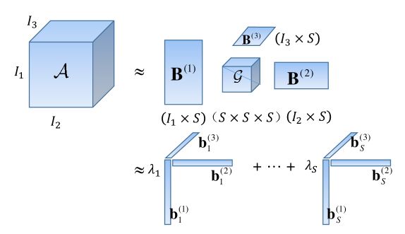
Figure 1: An example of CP decomposition.

Definition 10

(Tucker decomposition 33 ; 34 ; 35 ; 32 ) For a multiway array $\mathcal{A}\in\mathbb{R}^{I_{1}\times\cdots\times I_{N}}$, the Tucker decomposition is defined as

$$\mathcal{A} = \sum_{s_{1}=1}^{S_{1}}\times\sum_{s_{N}=1}^{S_{N}}g_{s_{1}s_{2}\dots s_{N}}(\mathbf{b}_{s_{1}}^{(1)}\circ\mathbf{b}_{s_{2}}^{(1)}\circ\dots\circ\mathbf{b}_{s_{N}}^{(N)})$$

$$= \mathcal{G}\times_{1}\mathbf{B}^{(1)}\times_{2}\mathbf{B}^{(2)}\dots\times_{N}\mathbf{B}^{(N)},$$

where $\mathcal{G}\in\mathbb{R}^{S_{1}\times S_{2}\times\dots\times S_{N}}$, $\mathbf{B}^{(n)}=[\mathbf{b}_{1}^{(n)},\mathbf{b}_{2}^{(n)},\dots,\mathbf{b}_{S}^{(n)}]\in\mathbb{R}^{I_{n}\times S_{n}}$ and the rank of Tucker representation is defined as $\operatorname{rank}_{\operatorname{Tucker}}(\mathcal{A})=(S_{1},S_{2},\cdots,S_{N})$. The detailed illustration of 3-order Tucker decomposition can be seen in Fig. 2.

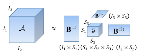
Figure 2: An example of Tucker decomposition.

Definition 11

(Tensor permutation) For a multiway array $\mathcal{X}\in\mathbb{R}^{I_{1}\times\cdots\times I_{N}}$, the tensor permutation is defined as $\mathcal{X}^{P_{n}}\in\mathbb{R}^{I_{n}\times\cdots\times I_{N}\times I_{1}\cdots\times I_{n-1}}$:

$$\mathcal{X}^{P_{n}}(i_{n},\cdots,i_{N},i_{1},\cdots,i_{n-1})=\mathcal{X}(i_{1},\cdots,i_{N}).$$

Definition 12

(Tensor train decomposition 36 ) For a multiway array $\mathcal{A}\in\mathbb{R}^{I_{1}\times\cdots\times I_{N}}$, the tensor train decomposition is defined as

$$\mathcal{A}(i_{1},i_{2},\cdots,i_{N})=\mathcal{U}_{1}(:,i_{1},:)\mathcal{U}_{2}(:,i_{2},:)\cdots\mathcal{U}_{N}(:,i_{N},:),$$

where the $\mathcal{U}_{n}\in\mathbb{R}^{S_{n}\times I_{n}\times S_{n+1}}$, $n=1,\cdots,N$ are the cores, and the rank of tensor train representation is defined as $\operatorname{rank}_{\operatorname{TT}}(\mathcal{A})=(S_{1},S_{2},\cdots,S_{N+1})$ with $S_{1}=S_{N+1}=1$. The graphical of tensor train decomposition can be seen in Fig. 3.

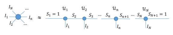
Figure 3: An example of Tensor train decomposition.

Definition 13

(Tensor ring decomposition) 37 For a multiway array $\mathcal{A}\in\mathbb{R}^{I_{1}\times\cdots\times I_{N}}$, the tensor ring decomposition is defined as

$$\mathcal{A}(i_{1},i_{2},\cdots,i_{N})=tr(\mathcal{U}_{1}(:,i_{1},:)\mathcal{U}_{2}(:,i_{2},:)\cdots\mathcal{U}_{N}(:,i_{N},:)),$$

where the $\mathcal{U}_{n}\in\mathbb{R}^{S_{n}\times I_{n}\times S_{n+1}}$, $n=1,\cdots,N$ are the cores, and the rank of tensor ring representation is defined as $\operatorname{rank}_{\operatorname{TR}}(\mathcal{A})=(S_{1},S_{2},\cdots,S_{N})$ and $S_{N+1}=S_{1}$. The graphical of tensor ring decomposition can be seen in Fig. 4.

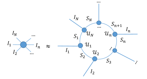
Figure 4: An example of Tensor ring decomposition.

Tensor train is a special case of tensor ring when $S_{1}=1$, we treated these two decomposition as a simple tensor network decomposition format. For an efficient representation of tensor network decomposition, we first introduce a tensor product between 3-order tensors, called tensor connection product.

Before that, the left and right unfoldings of the factors in tensor train decomposition are denoted as:

$${\bf{U}}_{n}^{\operatorname{L}} = ({\bf{U}}_{n})_{<2>}\in\mathbb{R}^{S_{n}I_{n}\times S_{n+1}},$$

$${\bf{U}}_{n}^{\operatorname{R}} = ({\bf{U}}_{n})_{<1>}\in\mathbb{R}^{S_{n}\times I_{n}S_{n+1}}.$$

Definition 14

(Tensor connection product) 38 The tensor connection product for $N$ 3-order tensors $\mathcal{U}_{n}\in\mathbb{R}^{S_{n}\times I_{n}\times S_{n+1}}$ is defined as

$$\mathcal{U}=\mathcal{U}_{1}\mathcal{U}_{2}\cdots\mathcal{U}_{N}\in\mathbb{R}^{S_{1}\times(I_{1}\cdots I_{N})\times S_{N+1}},$$

where $\mathcal{U}_{n}\mathcal{U}_{n+1}\in\mathbb{R}^{S_{n}\times(I_{n}I_{n+1})\times S_{n+2}}$ satisfies

$$\mathcal{U}_{n}\mathcal{U}_{n+1}=\operatorname{reshape}({\bf{U}}_{n}^{\operatorname{L}}{\bf{U}}_{n+1}^{\operatorname{R}},[S_{n},I_{n}I_{n+1},S_{n+2}])$$

for $n=1,\cdots,N$, where $\operatorname{reshape}$ is a reshaping operation from a matrix of the size $S_{n}I_{n}\times I_{n+1}S_{n+2}$ to a tensor of the size $S_{n}\times(I_{n}I_{n+1})\times S_{n+2}$.

Then simple tensor network decomposition can be represented as $\mathcal{A}=f(\mathcal{U})=f(\mathcal{U}_{1}\mathcal{U}_{2}\cdots\mathcal{U}_{N})$, where function $f$ is a trace operation on $\mathcal{U}(:,i,:)$, $i=1,\cdots,I_{1}I_{2}\cdots I_{N}$, and followed by a reshaping operation from vector of the size $1\times(I_{1}I_{2}\cdots I_{N})\times 1$ to tensor of the size $I_{1}\times I_{2}\times\cdots\times I_{N}$.

Theorem 2.1

(Cyclic permutation property) Based on the definition of tensor permutation and tensor train decomposition, the tensor permutation of $\mathcal{A}$ is equivalent to the cyclic permutation of its factors in tensor train decomposition form:

$$\mathcal{A}^{P_{n}}=f(\mathcal{U}_{n}\cdots\mathcal{U}_{N}\mathcal{U}_{1}\cdots\mathcal{U}_{n-1}),$$

with entries

$$\mathcal{A}^{P_{n}}(i_{n},\cdots,i_{N},i_{1},\cdots,i_{n-1})=\operatorname{Trace}(\mathcal{U}_{n}(:,i_{n},:)\cdots$$

$$\quad\quad\mathcal{U}_{N}(:,i_{N},:)\mathcal{U}_{1}(:,i_{1},:)\cdots\mathcal{U}_{n-1}(:,i_{n-1},:)).$$

Definition 15

(t-product 39 ) For multiway arrays $\mathcal{A}\in\mathbb{R}^{I_{1}\times I_{2}\times I_{3}}$ and $\mathcal{B}\in\mathbb{R}^{I_{2}\times I_{4}\times I_{3}}$, the t-product can be defined as:

$$\mathcal{C}=\mathcal{A}\ast\mathcal{B}\in\mathbb{R}^{I_{1}\times I_{4}\times I_{3}}$$

with

$$\mathcal{C}(i_{1},i_{4},:)=\sum\limits_{i_{2}=1}^{I_{2}}\mathcal{A}(i_{1},i_{2},:)\bullet\mathcal{B}(i_{2},i_{4},:),$$

where $\bullet$ denotes the circular convolution between two tubes of same size.

Definition 16

(conjugate transpose) 40 The conjugate transpose of a tensor $\mathcal{A}$ of size $\emph{I}_{1}\times\emph{I}_{2}\times\emph{I}_{3}$ is the $\emph{I}_{2}\times\emph{I}_{1}\times\emph{I}_{3}$ tensor $\mathcal{A}^{\mathrm{T}}$ obtained by conjugate transposing each of the frontal slice and then reversing the order of transposed frontal slices from 2 to $\emph{I}_{3}$.

Definition 17

(t-SVD 40 ) For a tensor $\mathcal{A}\in\mathbb{R}^{I_{1}\times I_{2}\times I_{3}}$ , the t-SVD of $\mathcal{A}$ is given by

$$\mathcal{A}=\mathcal{U}*\mathcal{S}*\mathcal{V^{\mathrm{T}}}$$

where $\mathcal{U}\in\mathbb{R}^{I_{1}\times I_{1}\times I_{3}}$ and $\mathcal{V}\in\mathbb{R}^{I_{2}\times I_{2}\times I_{3}}$ satisfy $\mathcal{U}\ast\mathcal{U}^{T}=\mathcal{U}^{T}\ast\mathcal{U}=\mathcal{I}\in\mathbb{R}^{I_{1}\times I_{1}\times I_{3}}$and $\mathcal{V}\ast\mathcal{V}^{T}=\mathcal{V}^{T}\ast\mathcal{V}=\mathcal{I}\in\mathbb{R}^{I_{2}\times I_{2}\times I_{3}}$ respectively, and $\mathcal{S}\in\mathbb{R}^{I_{1}\times I_{2}\times I_{3}}$ is a f-diagonal tensor whose frontal slices ia a diagonal matrix.

We can obtain this decomposition by computing matrix singular value decomposition (SVD) in the Fourier domain, as it shows in Algorithm 1. Fig. 4 illustrates the decomposition for the three-dimensional case.

$\bf Algorithm1:$ t-SVD for 3-way data

Input: $\mathcal{A}\in\mathbb{R}^{I_{1}\times I_{2}\times I_{3}}$

$\mathcal{D}\leftarrow$fft($\mathcal{A}$,[],$3$),

$\bf for$ $i=1$ to $I_{3}$, do

$[$ U , S , V $]$ = svd$(\mathcal{D}(:,:,i))$,

$\hat{\mathcal{U}}(:,:,i)$=$\bf U$,  $\hat{\mathcal{S}}(:,:,i)$)=$\bf S$,  $\hat{\mathcal{V}}(:,:,i)$ =$\bf V$,

end for

$\mathcal{U}\leftarrow$ ifft($\hat{\mathcal{U}}$,[],3),  $\mathcal{S}\leftarrow$ ifft($\hat{\mathcal{S}}$,[],3),  $\mathcal{V}\leftarrow$ ifft($\hat{\mathcal{V}}$,[],3),

Output: $\mathcal{U},\mathcal{S},\mathcal{V}$

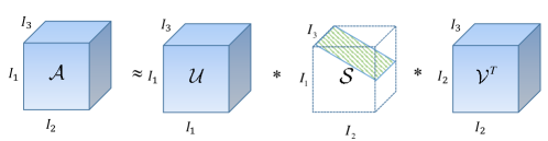
Figure 5: Illustration of the t-SVD of an $I_{1}\times I_{2}\times I_{3}$ tensor.

3 Matrix Completion

Matrix completion is the problem of recovering a data matrix from its partial entries. In many problems, we often assume that the matrix, which we wish to recover, is low rank or approximately low rank. The optimization model for matrix completion was proposed firstly in 19 , and can be formulated as:

$$\operatorname*{minimize}_{\mathbf{X}}\quad\operatorname{rank}(\mathbf{X})$$

$$\text{subject to}\quad\mathbf{X}_{\mathbb{O}}=\mathbf{T}_{\mathbb{O}},$$ (1)

where $\mathbf{X}$ represents the completed low-rank matrix, the $\operatorname{rank}(\mathbf{X})$ is equal to the rank of the matrix $\mathbf{X}$ and the $\mathbb{O}$ is the entries sets. The equality constraint $\mathbf{X}_{\mathbb{O}}=\mathbf{T}_{\mathbb{O}}$ means that the available entries in observation matrix $\mathbf{T}$ is equal to the available entries in completed matrix $\mathbf{X}$. This optimization problem is NP-hard, and can be solved by some fundamental matrix completion approaches. These methods could be divided into two categories : minimize matrix nuclear norm and low rank matrix decomposition.

3.1 nuclear norm based matrix completion

In solving the matrix completion problems, we can use matrix nuclear norm replace non-convex rank function as a convex surrogate. It has been proven that matrix nuclear norm is the tightest lower bound of matrix rank function among all possible convex 26 . The optimization problem (1) can be written as:

$$\operatorname*{minimize}_{\mathbf{X}}\quad\lVert\mathbf{X}\rVert_{*}$$

$$\text{subject to }\quad\mathbf{X}_{\mathbb{O}}=\mathbf{T}_{\mathbb{O}},$$ (2)

where the nuclear norm is defined as $\lVert\mathbf{X}\rVert_{*}=\sum_{i=1}^{\operatorname{min}\{M,N\}}\sigma_{i}$, $\sigma_{i}$ is the singular value of $\mathbf{X}$, which can be obtained by singular value decomposition (SVD).

The singular value thresholding (SVT) algorithm can solve problem (2) by singular value shrinkage operator, which is defined as:

$$\operatorname{SVT}_{\tau}(\mathbf{X})=\mathbf{U}\operatorname{sth}_{\tau}(\Sigma)\mathbf{V}^{\text{T}},$$

where $\mathbf{U}$ and $\mathbf{V}$ are the right singular vectors and left singular vectors, respectively. $\operatorname{sth}_{\tau}$ is the well-known soft thresholding operator as follows:

$$\operatorname{sth}_{\tau}=\operatorname{sgn}(x)\text{max}(\lvert x\rvert-\tau,0).$$

With $\tau>0$ and a sequence of scalar step sizes ${\delta}\geq 1$, $\mathbf{Y}^{0}$, the algorithm defines 20 :

$$\mathbf{X}^{k}=\operatorname{SVT}_{\tau}(\mathbf{Y}^{k-1})$$

$$\mathbf{Y}^{k}=\mathbf{Y}^{k-1}+\delta(\mathbf{T}_{\mathbb{O}}-\mathbf{X}_{\mathbb{O}}^{k}),$$ (3)

until a stopping criterion is reached.

Another method to tackle the problem (2) is that add an additional variable matrix $\mathbf{M}$ and obtain the following equivalent formulation 27 :

$$\operatorname*{minimize}_{\mathbf{M}}\quad\lVert\mathbf{M}\rVert_{*}$$

$$\text{subject to }\quad\mathbf{M}=\mathbf{X},\quad\mathbf{X}_{\mathbb{O}}=\mathbf{T}_{\mathbb{O}}.$$ (4)

Then we define the following augment Lagrangian function:

$$\operatorname*{minimize}_{\mathbf{M}}\quad\lVert\mathbf{M}\rVert_{*}+\langle\Lambda,\mathbf{M}-\mathbf{X}\rangle+\frac{\beta}{2}\lVert\mathbf{M}-\mathbf{X}\rVert_{\text{F}}^{2}$$

$$\text{subject to }\quad\mathbf{X}_{\mathbb{O}}=\mathbf{T}_{\mathbb{O}},$$ (5)

and according to the alternating direction method of multipliers (ADMM) 41 framework, one can iteratively update $\mathbf{M}$, $\mathbf{X}$, and $\Lambda$, with the initial values $\mathbf{X}_{\mathbb{O}}^{0}=\mathbf{T}_{\mathbb{O}}$ and $\mathbf{X}_{\bar{\mathbb{O}}}=0$ , the algorithm can be formulated as:

$$\mathbf{M}^{k}=\operatorname{D}_{\frac{1}{\beta}}(\mathbf{X}^{k-1}+\frac{1}{\beta}\Lambda^{k-1})$$

$$\mathbf{X}_{\bar{\mathbb{O}}}^{k}=(\mathbf{M}^{k}-\frac{1}{\beta}\Lambda^{k-1})_{\bar{\mathbb{O}}}$$

$$\Lambda^{k}=\Lambda^{k-1}-\beta(\mathbf{M}^{k}-\mathbf{X}^{k}),$$ (6)

until a stopping criterion is reached.

3.2 low rank matrix decomposition based matrix completion

It’s known that SVD becomes increasingly costly as the sizes of the underlying matrices increase, so nuclear norm based algorithms should bear the computational cost required by SVD. It is therefore desirable to exploit an alternative approach that avoids SVD computation all together, by replacing it with some less expensive computation. Hence, a non-SVD approach in order to more efficiently solve large-scale matrix completion problems has been proposed.

Based on the low rank matrix decomposition model, the problem (1) can be converted into 24 :

$$\operatorname*{minimize}_{\mathbf{X},\mathbf{Y},\mathbf{Z}}\quad\frac{1}{2}\lVert\mathbf{X}\mathbf{Y}-\mathbf{Z}\rVert_{\text{F}}^{2}$$

$$\text{subject to}\quad\mathbf{Z}_{\mathbb{O}}=\mathbf{T}_{\mathbb{O}},$$ (7)

where $\mathbf{X}\in\mathbb{R}^{m\times S}$, $\mathbf{Y}\in\mathbb{R}^{S\times n}$, $\mathbf{Z}\in\mathbb{R}^{m\times n}$, and the integer $S$ is the rank of matrix $\mathbf{Z}$. This problem can be solved by updating these three variables by minimizing (7) with respect to each one separately while fixing the other two. The updated algorithm is following iterative scheme:

$$\mathbf{X}^{k}=\mathbf{Z}^{k-1}(\mathbf{Y}^{k-1})^{\text{T}}(\mathbf{Y}^{k-1}(\mathbf{Y}^{k-1})^{\text{T}})^{\dagger}$$

$$\mathbf{Y}^{k}=((\mathbf{X}^{k})^{\text{T}}\mathbf{X}^{k})^{\dagger}((\mathbf{X}^{k})^{\text{T}}\mathbf{Z}^{k})$$

$$\mathbf{Z}^{k}=(\mathbf{X}^{k}\mathbf{Y}^{k})_{\bar{\mathbb{O}}}+\mathbf{T}_{\mathbb{O}}$$ (8)

4 Tensor Completion

Tensor is the generalization of the matrix. Tensor completion is defined as a problem of completing an $N$-th order tensor $\mathcal{X}\in{\mathbb{R}^{I_{1}\times I_{2}\cdots\times I_{N}}}$ from its known entries given by an index set $\mathbb{O}$. In recent literature, the successful recovery of tensor completion mainly relies on its low rank assumption. The methods for tensor completion include two kinds of approaches. One is based on a given rank and update factors in tensor completion. The one directly minimizes the tensor rank and updates the low-rank tensor.

The main framework of this chapter can be illustrated by Fig. 6.

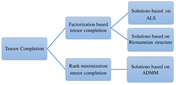
Figure 6: The outline of this chapter.

4.1 Factorization based approaches

In this section, we demonstrate the tensor completion based on a given rank bound with different tensor decomposition methods in detail. The optimization problem of tensor completion with a given rank bound can be formulated as:

$$\operatorname*{minimize}_{\mathcal{X}}\quad\frac{1}{2}\lVert\mathcal{P}_{\mathbb{O}}(\mathcal{X}-\mathcal{T})\rVert_{\text{F}}^{2}$$

$$\text{subject to}\quad\operatorname{rank(\mathcal{X})}=S,$$ (9)

where $\mathcal{X}$ is the recovered tensor, and $\mathcal{T}$ is the observed tensor. $\operatorname{rank}(\mathcal{X})$ has different forms, such CP rank, Tucker rank, tensor train rank, tensor ring rank, etc. $S$ is a given bound rank of low rank $\mathcal{X}$, and $\mathcal{P}_{\mathbb{O}}$ denotes the random sampling operator, which is defined by:

$$\mathcal{P}_{\mathbb{O}}(\mathcal{A})=\left\{\begin{array}[]{rcl}\mathcal{A}_{i_{1},i_{2},\dots,i_{N}}&&(i_{1},i_{2},\dots,i_{N})\in\mathbb{O}\\ 0&&\text{otherwise}.\end{array}\right.$$

CP factorization based approaches

Given a tensor $\mathcal{X}\in\mathbb{R}^{I_{1}\times I_{2}\dots\times I_{N}}$ with a known CP rank, which denotes the number of rank-one tensor, the (9) can be formulated as the following optimization problem 42 :

$$\operatorname*{minimize}_{\mathcal{X},\mathbf{B}^{(n)}}\quad\frac{1}{2}\lVert\mathcal{P}_{\mathbb{O}}(\mathcal{X}-\mathcal{T})\rVert_{\text{F}}^{2}$$

$$\text{subject to}\quad\mathcal{X}=\sum_{s=1}^{S}\lambda_{s}\mathbf{b}_{s}^{(1)}\circ\mathbf{b}_{s}^{(2)}\circ\dots\circ\mathbf{b}_{s}^{(N)}.$$ (10)

This problem can be solved by the alternating least squares (ALS), which updates one variable with other variables fixed 42 . However, the model is non-convex, which would suffer from the local-minimum and need a good initialization to perform well 43 . Besides, some other related methods such as CP weighted optimization (CPWOPT) 44 , Geometric nonlinear conjugate gradient (geomCG) 45 are proposed to deal with this problem.

Recently, some methods can improve the recovery results through the data prior information. As far as we know, there are mainly two methods that consider the data patterns. One is fully Bayesian CANECOMP/PARAFAC (FBCP) method 46 , which uses the Bayesian inference to find an appropriate tensor rank. The joint distribution of this framework can be written as:

$$p(\mathcal{T}_{\mathbb{O}},\Theta)=p(\mathcal{T}_{\mathbb{O}}|\{\mathbf{B}^{(n)}\}_{n=1}^{N},\tau)\prod_{n=1}^{N}p(\mathbf{B}^{(n)}|\bm{\lambda})p(\bm{\lambda})p(\tau)$$ (11)

where the hyperparameters $\Theta=\{B^{(1)},B^{(2)},\dots,B^{(N)},\bm{\lambda,\tau}\}$, $\bm{\lambda}=[\lambda_{1},\lambda_{2},\dots,\lambda_{S}]$, $\tau$ denotes the noise precision. The hyperprior over $\bm{\lambda}$ can be defined by:

$$p(\bm{\lambda})=\prod_{s=1}^{S}\Gamma(\lambda_{s}|a,b),$$

where $\Gamma(x|a,b)=\frac{b^{a}x^{a-1}e^{-bx}}{\Gamma(a)}$ is a Gamma distribution.

The other is smooth PARAFAC tensor completion (SPC) method 47 , which can be formulated as:

$$\operatorname*{minimize}_{g_{1},\cdots,g_{S},\mathbf{u}^{(1)},\ldots,\mathbf{u}^{(N)}}\frac{1}{2}\Arrowvert\mathcal{X}-\mathcal{Y}\Arrowvert_{\text{F}}^{2}+\sum_{s=1}^{S}\frac{g_{s}^{2}}{2}\sum_{n=1}^{N}\rho^{(n)}\Arrowvert\mathbf{L}^{(n)}\mathbf{u}_{s}^{(N)}\Arrowvert_{p}^{p},$$

$$\text{subject to}~{}\mathcal{Y}=\sum_{s=1}^{S}g_{s}\mathbf{u}_{s}^{(1)}\circ\mathbf{u}_{s}^{(2)}\circ\cdots\circ\mathbf{u}_{s}^{(n)},~{}\mathcal{X}_{\mathbb{O}}=\mathcal{Z}_{\mathbb{O}},~{}\mathcal{X}_{\mathbb{O}}=\mathcal{Y}_{\mathbb{O}},$$

$$\Arrowvert\mathbf{u}_{s}^{(N)}\Arrowvert_{2}=1,~{}\forall s\in\{1,\ldots,S\},~{}\forall n\in\{1,\ldots,N\}.$$ (12)

where $g_{s}$ is a coefficient of the $s$-th rank-one factor tensor in CP decompostion, $\mathbf{u}_{s}^{(n)}$ is $r$-th feature vector, $\circ$ is the outer product of vectors, $\Arrowvert\mathbf{L}^{(n)}\mathbf{u}_{s}^{(n)}\Arrowvert_{p}^{p}$ is a smoothness term, which can be divided into two kinds of total variations. When $p=1$, the term is total variation (TV) and when $p=2$, the constraint term is quadratic variation (QV).

Tucker factorization based approaches

Given a tensor $\mathcal{X}\in\mathbb{R}^{I_{1}\times I_{2}\dots\times I_{N}}$ with a known Tucker rank $(S_{1},S_{2},\dots,S_{N})$, the (9) can be formulated as the following optimization problem 48 :

$$\operatorname*{minimize}_{\mathcal{X},\mathbf{B}^{(n)},\mathcal{G}}\quad\frac{1}{2}\lVert\mathcal{P}_{\mathbb{O}}(\mathcal{X}-\mathcal{T})\rVert_{\text{F}}^{2}$$

$$\text{subject to}\quad\mathcal{X}=\mathcal{G}\times_{1}\mathbf{B}^{(1)}\times_{2}\mathbf{B}^{(2)}\dots\times_{N}\mathbf{B}^{(N)},$$ (13)

where $\mathcal{G}\in\mathbb{R}^{S_{1}\times S_{2}\times\dots\times S_{N}}$ is the core tensor, and the factor matrix $\mathbf{B}^{(n)}\in\mathbb{R}^{I_{n}\times S_{n}}$. This problem can be solved by the ALS algorithm 48 and speeded by the high-order orthogonal iteration (HOOI) 32 ,which iteratively calculates one column-wise orthogonal factor matrix corresponding to the dominant singular vectors of $\mathbf{X}^{(n)}$. Besides, when the majority of the tensor entries are unknown, some related methods 45 ; 49 ; 50 are efficient. They exploit the Riemannian structure on the manifold tensors with known tucker rank and use nonlinear conjugate gradient descent.

In addition, the generalized model of tensor completion with a predefined Tucker rank is popular and can be formulated as:

$$\operatorname*{minimize}_{\mathcal{X}}\quad\frac{1}{2}\lVert\mathbf{t}-\mathcal{P}(\mathcal{X})\rVert_{\text{F}}^{2}$$

$$\text{subject to}\quad\operatorname{rank}_{\text{Tucker}}(\mathcal{X})\leq(S_{1},S_{2},\dots,S_{N}),$$ (14)

where $\mathbf{t}\in\mathbb{R}^{M}$ is the observation data, $\mathcal{P}:\mathbb{R}^{I_{1}\times I_{2},\dots\times I_{N}}\longmapsto\mathbb{R}^{M}$ is the linear measurement operator. This problem can be solved by tensor iterative hard thresholding (TIHT) 51 , which employs the truncated higher order singular value decomposition (HOSVD) 33 as the thresholding operator and achieves a quasi-optimal low rank tensor approximation. In  52 , an improved step size TIHI (ISS-TIHI) is proposed to increase the convergence speed. Besides, other related works such as sequentially optimal modal projections (SeMP) 53 , sequential rank-one approximation and projection (SeROAP) 54 , and sequential low-rank approximation and projection (SeLRAP) 55 are proposed to effectively resolve tensor recovery problems.

Tensor train factorization based approaches

Given a tensor $\mathcal{X}\in\mathbb{R}^{I_{1}\times I_{2}\dots\times I_{N}}$ with a known tensor train rank $(S_{1},S_{2},\dots,S_{N},S_{N+1})$, the (9) can be formulated as the following optimization problem 56 :

$$\operatorname*{minimize}_{\mathcal{X},\mathcal{U}}\quad\frac{1}{2}\lVert\mathcal{X}-\mathcal{Y}\rVert_{\text{F}}^{2}$$

$$\text{subject to}\quad\mathcal{P}_{\mathbb{O}}(\mathcal{X})=\mathcal{P}_{\mathbb{O}}(\mathcal{T}),\quad\mathcal{Y}\in\mathbb{T}_{\text{TT}}(S_{1},S_{2},\dots,S_{N}).$$ (15)

where $\mathcal{Y}\in\mathbb{T}_{\text{TT}}(S_{1},S_{2},\dots,S_{N})$ means $\mathcal{Y}(i_{1},i_{2},\cdots,i_{N})=\mathcal{U}_{1}(:,i_{1},:)\mathcal{U}_{2}(:,i_{2},:)\cdots\mathcal{U}_{N}(:,i_{N},:)$, $\mathcal{U}_{n}\in\mathbb{R}^{S_{n}\times I_{n}\times S_{n+1}}$. This problem is non-convex and exists a quasi-optimal approximation solution. It can be calculated using nonlinear block Gauss-Seidel iteration with respect to the blocks $\mathcal{U}_{1},\mathcal{U}_{2},\dots,\mathcal{U}_{N},\mathcal{X}$ 56 ; 57 . For each small block, it can be solved by least squares fit and this approach can accelerate the convergence by successive over-relaxation, which is called as alternating directions fitting  56 . Besides, with fixed tensor train rank, this problem can be solved using a nonlinear conjugate gradient scheme within the framework of Riemannian optimization58 , which can make the storage complexity scaling linear with the number of dimensions.

In addition, with the success of matrix completion 59 and tensor completion using Tucker rank 60 ; 61 , a similarly way of tensor completion using fixed tensor train rank bound was proposed in the form of 62 :

$$\operatorname*{minimize}_{\mathbf{U}_{n},\mathbf{V}_{n},\mathcal{X}}\quad\sum_{n=1}^{N-1}\frac{\alpha_{n}}{2}\lVert\mathbf{U}_{n}\mathbf{V}_{n}-\mathbf{X}_{<n>}\rVert_{\text{F}}^{2}$$

$$\text{subject to}\quad\mathcal{P}_{\mathbb{O}}(\mathcal{X})=\mathcal{P}_{\mathbb{O}}(\mathcal{T})$$ (16)

where $\mathbf{X}_{<n>}\in\mathbb{R}^{\prod_{j=1}^{n}I_{j}\times\prod_{j=n+1}^{N}I_{j}}$. With a given rank $S_{n}$, the matrix $\mathbf{X}_{<n>}$ can be factorized as $\mathbf{X}_{<n>}=\mathbf{U}_{n}\mathbf{V}_{n}$ with $\mathbf{U}_{n}\in\mathbb{R}^{\prod_{j=1}^{n}I_{j}\times S_{n}}$ and $\mathbf{V}_{n}\in\mathbb{R}^{S_{n}\times\prod_{j=n+1}^{N}I_{j}}$. For this problem, the block coordinate descent (BCD) method 63 was used to optimize to alternatively optimize different groups of variables ($\mathbf{U}_{n},\mathbf{V}_{n},\mathcal{X}$).

Tensor Ring factorization based approaches

To the best of our knowledge, low rank tensor ring completion 64 is the only one work for tensor completion with fixed tensor ring rank $(S_{1},S_{2},\dots,S_{N})$. Given a tensor $\mathcal{X}\in\mathbb{R}^{I_{1}\times I_{2}\dots\times I_{N}}$ under tensor ring model, the optimization problem can be formulated as:

$$\operatorname*{minimize}_{\mathcal{U}}\quad\frac{1}{2}\lVert\mathcal{P}_{\mathbb{O}}(\mathcal{X}-\mathcal{T})\rVert_{\text{F}}^{2}$$

$$\text{subject to}\quad\mathcal{X}\in\mathbb{T}_{\text{TR}}(S_{1},S_{2},\dots,S_{N}).$$ (17)

where $\mathcal{X}\in\mathbb{T}_{\text{TR}}(S_{1},S_{2},\dots,S_{N})$ means $\mathcal{X}(i_{1},i_{2},\cdots,i_{N})=\operatorname{tr}(\mathcal{U}_{1}(:,i_{1},:)\mathcal{U}_{2}(:,i_{2},:)\cdots\mathcal{U}_{N}(:,i_{N},:))$, $\mathcal{U}_{n}\in\mathbb{R}^{S_{n}\times I_{n}\times S_{n+1}}$. The tensor train ranks present the distribution of the large for the middle factors and the lower for the boarder factors. And in fact, the closer to the boarder factor, the lower the tensor train ranks are. The tensor train decomposition drawbacks can be alleviate by tensor ring factorization. The optimization problem (17) can be solved by ALS with a good initial point choosing. In 64 , the author proposed a novelty initialization algorithm which called tensor ring approximation to make sure the ALS algorithm performs well.

t-SVD factorization based approaches

In this section, we consider a tensor $\mathcal{X}\in\mathbb{R}^{I_{1}\times I_{2}\times I_{3}}$ with a fixed tubal rank. The optimization problem of low tubal rank tensor completion problem can be formulated as:

$$\operatorname*{minimize}_{\mathcal{X}\in\mathbb{R}^{I_{1}\times I_{2}\times I_{3}}}\quad\lVert\mathcal{P}_{\mathbb{O}}(\mathcal{X}-\mathcal{T})\rVert_{\text{F}}$$

$$\text{subject to}\quad\operatorname{rank(\mathcal{X})}\leq S,$$ (18)

This problem can be solved by decomposing the target tensor as the circular convolution of two low tubal rank tensor, which can be rewritten as 65 :

$$\operatorname*{minimize}_{\mathcal{X},\mathcal{A},\mathcal{B}}\quad\lVert\mathcal{P}_{\mathbb{O}}(\mathcal{A}\ast\mathcal{B}^{\dagger}-\mathcal{T})\rVert_{\text{F}}$$

$$\text{subject to}\quad\mathcal{X}=\mathcal{A}\ast\mathcal{B}^{\dagger}$$ (19)

where $\mathcal{A}\in\mathbb{R}^{I_{1}\times S\times I_{3}},\mathcal{B}\in\mathbb{R}^{I_{2}\times S\times I_{3}}$. This low tubal rank tensor completion model can be solved by alternating minimization algorithm 24 ; 66 .

Furthermore, a tensor-CUR decomposition based model was proposed to solve the problem (18), which can be converted to the following optimization problem 67 :

$$\operatorname*{minimize}_{\mathcal{U}}\quad\lVert\mathcal{P}_{\mathbb{O}}(\mathcal{C}\ast\mathcal{U}\ast\mathcal{R}-\mathcal{T})\rVert_{\text{F}}$$

$$\text{subject to}\quad\mathcal{X}=\mathcal{C}\ast\mathcal{U}\ast\mathcal{R},\quad\mathcal{P}_{\mathbb{O}}(\mathcal{X})=\mathcal{P}_{\mathbb{O}}(\mathcal{T})$$ (20)

where $\mathcal{C}\in\mathbb{R}^{I_{1}\times I_{1}\times I_{3}}$, $\mathcal{U}\in\mathbb{R}^{I_{1}\times I_{2}\times I_{3}}$, $\mathcal{R}\in\mathbb{R}^{I_{2}\times I_{2}\times I_{3}}$. It can be solved by the matrix-CUR approximation for each frontal face. Besides, In 68 , the authors show the smooth manifold of a fixed tubal rank tensor can be seen as an element of the product manifold of fixed low-rank matrices in the Fourier domain. This problem can be solved by the traditional convex methods such as conjugate gradient descent 69 .

4.2 Rank minimization model

In practice, the tensor rank bounds may not be available in some applications. When only a few observations are available, the choice of high rank bound may led to over-fitting. To avoid the occurrence of it, another group of methods is to directly minimize the tensor rank, which can be given as follows:

$$\operatorname*{minimize}_{\mathcal{X}}\quad\operatorname{rank}(\mathcal{X})$$

$$\text{subject to}\quad\mathcal{X}_{\mathbb{O}}=\mathcal{T}_{\mathbb{O}},$$ (21)

where $\mathcal{X}_{\mathbb{O}}=\mathcal{T}_{\mathbb{O}}$ means the $\mathcal{X}_{i_{1},\dots,i_{N}}=\mathcal{T}_{i_{1},\dots,i_{N}}$, the index $\{i_{1},\dots,i_{N}\}$ is in the observation index $\mathbb{O}$, where $\operatorname{rank}(\mathcal{X})$ denotes the rank of tensor variable $\mathcal{X}$. There are different kinds of tensor ranks, such as CP rank, Tucker rank, tubal rank, tensor train rank, etc. With different definitions of tensor rank, there are many methods optimization models for tensor completion problems. However, the rank is a non-convex function with respect to $\mathcal{X}$, and the problem (21) is NP-hard 70 . Most existing methods 71 ; 72 are using nuclear norm (trace norm) as the convex surrogate of non-convex rank function. In particular, the tensor nuclear norm for CP rank is impossible to solve and to the best of our knowledge, tensor nuclear norm for tensor ring rank has never been investigated for tensor completion. Hence, we will mainly introduce the methods of Tucker rank minimization, tubal rank minimization and tensor train rank minimization for tensor completion in the following subsections.

Tucker rank minimization model

Given a tensor $\mathcal{X}\in\mathbb{R}^{I_{1}\times I_{2}\dots\times I_{N}}$, the tensor completion based on minimizing Tucker rank can be formulated as:

$$\operatorname*{minimize}_{\mathcal{X}}\quad\operatorname{rank}_{\text{Tucker}}(\mathcal{X})$$

$$\text{subject to}\quad\mathcal{X}_{\mathbb{O}}=\mathcal{T}_{\mathbb{O}},$$ (22)

where $\operatorname{rank}_{\text{Tucker}}(\mathcal{X})=(\operatorname{rank}(\mathbf{X}_{[1]}),\operatorname{rank}(\mathbf{X}_{[2]}),\dots,\operatorname{rank}(\mathbf{X}_{[N]})$ 32 , and $\operatorname{rank}(\mathbf{X}_{[n]})$ denotes the rank of the unfolding matrix $\mathbf{X}_{[n]}$. Under the definition of Tucker rank, the optimization problem (22) can be written as 73 ; 74 ; 60 :

$$\operatorname*{minimize}_{\mathbf{X}_{[n]}}\quad\sum^{N}_{n=1}w_{n}\operatorname{rank}(\mathbf{X}_{[n]})$$

$$\text{subject to}\quad\mathcal{X}_{\mathbb{O}}=\mathcal{T}_{\mathbb{O}},$$ (23)

where $w_{n},n=1,\cdots,N$ are the weights with $\sum^{N}_{n=1}w_{n}=1$. In fact, the matrix rank functions in the optimization model (4.2) is nonconvex, but it can be relaxed to the matrix nuclear norm approximation. This generates the following optimization problem 73 :

$$\operatorname*{minimize}_{\mathbf{X}_{[n]}}\quad\sum^{N}_{n=1}w_{n}\Arrowvert\mathcal{X}_{[n]}\Arrowvert_{*}$$

$$\text{subject to}\quad\mathcal{X}_{\mathbb{O}}=\mathcal{T}_{\mathbb{O}}.$$ (24)

Where $\Arrowvert\mathcal{X}_{[n]}\Arrowvert_{*}$ is the tightest convex envelop for $\operatorname{rank}(\mathbf{X}_{[n]})$. The problem (4.2) can be solved using simple low-rank tensor completion (SiLRTC) and strictly solved using high accuracy low-rank tensor completion (HaLRTC) by adding an equation constraint 73 . In order to improve the performance, the method which uses volume measurement 75 is proposed and can be formulated as:

$$\operatorname*{minimize}_{\mathcal{X}}\quad\lVert\mathcal{X}\rVert_{\text{vol}}$$

$$\text{subject to}\quad\mathcal{X}_{\mathbb{O}}=\mathcal{T}_{\mathbb{O}},$$ (25)

where the volume of tensor is defined as:

$$\lVert\mathcal{X}\rVert_{\text{vol}} = \prod_{i=1}^{N}\lVert\mathbf{X}_{[i]}\rVert_{\text{vol}}$$

$$= \prod_{i=1}^{N}\prod_{j=1}^{N_{i}}\sigma_{j}(\mathbf{X}_{[i]}),$$

$\sigma_{j}(\mathbf{X}_{[i]})$ is the $j$-th singular value of mode-i unfolding matrix. This model can be solved by the ADMM. However, the sum of weighted nuclear norms model may be sub-optimal with the dimension increasing 76 ; 77 . To handle the issue, a more appropriate convex model, which makes the mode-n unfolding matrix more balanced and maintains the low rank property was proposed 76 . In addition, the core tensor trace-norm minimization (CTNM) 78 method using ADMM algorithm can alleviate computational cost in large scale problems.

Furthermore, in order to enhance the recovery quality for some real data, such as natural images, videos, magnetic resonance imaging (MRI) images and hyperspectral images, investigating the intrinsic structure of data is necessary. Hence, some smooth priors can be added to improve the recovery quality for images completion 79 ; 80 ; 81 . There are two groups of state-of-the-art models for tensor completion considering the prior information.

Based on the factor prior, one presents the nuclear norm of individual factor matrices as the following optimization problem:

$$\operatorname*{minimize}_{\mathcal{X},\mathcal{G},\mathbf{U}^{(n)}}\quad\sum_{n=1}^{N}w_{n}\lVert\mathbf{U}^{(n)}\rVert_{*}+\beta\operatorname{tr}((\mathbf{U}_{1}\otimes\dots\otimes\mathbf{U}_{N})\mathbf{L}(\mathbf{U}_{1}\otimes\dots\otimes\mathbf{U}_{N})^{\text{T}})+\gamma\lVert\mathcal{G}\rVert_{\text{F}}^{2}$$

$$\text{subject to}\quad\mathcal{X}=\mathcal{G}\times_{1}\mathbf{U}_{1}^{\text{T}}\dots\times_{n}\mathbf{U}_{n}^{\text{T}},\quad\mathcal{X}_{\mathbb{O}}=\mathcal{T}_{\mathbb{O}}.$$ (26)

where $\beta\operatorname{tr}((\mathbf{U}_{1}\otimes\dots\otimes\mathbf{U}_{N})\mathbf{L}(\mathbf{U}_{1}\otimes\dots\otimes\mathbf{U}_{N})^{\text{T}})+\gamma\lVert\mathcal{G}\rVert_{\text{F}}^{2}$ are the regularization items, $\beta$ and $\gamma$ are the weighting parameters between nuclear norm and regularization items. $\mathbf{L}$ is a matrix designed by the prior information, and $\operatorname{tr}((\mathbf{U}_{1}\otimes\dots\otimes\mathbf{U}_{N})\mathbf{L}(\mathbf{U}_{1}\otimes\dots\otimes\mathbf{U}_{N})^{\text{T}})$ can be interpreted as the constraint for the local similarity of visual data. This problem can be solved using augmented Lagrange multiplier (ALM) algorithm 82 .

Based on the recovered tensor prior, the other proposes the simultaneous minimization of the tensor nuclear norm and total variation (TV). The optimization model is as follow:

$$\operatorname*{minimize}_{\mathcal{X}}\quad\lVert(1-\rho)\Arrowvert\mathcal{X}\Arrowvert_{*}+\rho\Arrowvert\mathcal{X}\Arrowvert_{\text{TV}}$$

$$\text{subject~{}to}~{}\nu_{\text{min}}\leq\mathcal{X}\leq\nu_{\text{max}},~{}\Arrowvert\mathcal{Z}_{\mathbb{O}}-\mathcal{X}_{\mathbb{O}}\Arrowvert_{\text{F}}^{2}\leq\delta.$$ (27)

where $\rho$ is the weight between nuclear norm and TV terms, and $\delta$ is the error bound.The first inequality constraint in (4.2) is to impose all values of output tensor within a given range [$\nu_{\text{min}}$,$\nu_{\text{max}}$]. The second inequality constraint implies that the recovered data entries and the observed data entries in the set $\mathbb{O}$ are generally consistent but allows existing a certain amount of noise. The problem of simultaneous minimization of low rank and TV terms can be solved by the primal-dual splitting method (LRTV-PDS) 80 ; 81 .

Tensor train rank minimization model

Given a tensor $\mathcal{X}\in\mathbb{R}^{I_{1}\times I_{2}\dots\times I_{N}}$, the tensor completion based on minimizing tensor train rank can be formulated as:

$$\operatorname*{minimize}_{\mathcal{X}}\quad\operatorname{rank}_{\text{TT}}(\mathcal{X})$$

$$\text{subject to}\quad\mathcal{X}_{\mathbb{O}}=\mathcal{T}_{\mathbb{O}},$$ (28)

where $\operatorname{rank}_{\text{TT}}(\mathcal{X})=(\operatorname{rank}(\mathbf{X}_{<1>}),\operatorname{rank}(\mathbf{X}_{<2>}),\dots,\operatorname{rank}(\mathbf{X}_{<N-1>})$ 36 , and $\operatorname{rank}(\mathbf{X}_{<n>})$ denotes the rank of the unfolding matrix $\mathbf{X}_{<n>}$, so it can be written as (28):

$$\operatorname*{minimize}_{\mathbf{X}_{<n>}}\quad\sum^{N-1}_{n=1}w_{n}\operatorname{rank}(\mathbf{X}_{<n>})$$

$$\text{subject to}\quad\mathcal{X}_{\mathbb{O}}=\mathcal{T}_{\mathbb{O}},$$ (29)

where $w_{n}$, $n=1,\cdots,N-1$ are the weights with $\sum_{n=1}^{N-1}w_{n}=1$. This optimization problem can be approximated by the matrix nuclear norm as follows 62 :

$$\operatorname*{minimize}_{\mathbf{X}_{<n>}}\quad\sum^{N-1}_{n=1}w_{n}\Arrowvert\mathbf{X}_{<n>}\Arrowvert_{*}$$

$$\text{subject to}\quad\mathcal{X}_{\mathbb{O}}=\mathcal{T}_{\mathbb{O}}.$$ (30)

Especially, the unfolding $\mathbf{X}_{<n>}$ is more balanced than the unfolding $\mathbf{X}_{[n]}$. For this model when $n=\frac{N}{2}$, it is similar to the case in 76 . The problem (4.2) can be solved by simple low-rank tensor completion via tensor train (SiLRTC-TT) 62 .

Tubal rank minimization model

Given a tensor $\mathcal{X}\in\mathbb{R}^{I_{1}\times I_{2}\times I_{3}}$, the tensor completion based on minimizing tensor tubal rank can be formulated as:

$$\operatorname*{minimize}_{\mathcal{X}}\quad\operatorname{rank}_{\text{tubal}}(\mathcal{X})$$

$$\text{subject to}\quad\mathcal{X}_{\mathbb{O}}=\mathcal{T}_{\mathbb{O}},$$ (31)

where the tensor tubal rank, denoted by $\mathrm{rank_{tubal}}(\mathcal{X})$, is the number of nonzero singular tubes of $\mathcal{S}$, where $\mathcal{S}$ is from $\mathcal{X}=\mathcal{U}*\mathcal{S}*\mathcal{V^{\mathrm{T}}}$ 83 . Following the optimization approach in 73 , the problem (31) is firstly formulated as 83 :

$$\operatorname*{minimize}_{\mathcal{X}}\quad\lVert\mathcal{X}\rVert_{\text{TNN}}$$

$$\text{subject to}\quad\mathcal{X}_{\mathbb{O}}=\mathcal{T}_{\mathbb{O}}$$ (32)

where $\lVert\mathcal{X}\rVert_{\text{TNN}}$ is the nuclear norm of $\mathcal{X}$, which is equal to the tensor nuclear norm (TNN ) of $\operatorname{blkdiag(\mathcal{\hat{X}})}$. Here $\text{blkdiag}(\mathcal{\hat{X}})$ is a block diagonal matrix defined as follows:

$$\mbox{blkdiag}(\hat{\mathcal{X}})=\left[\begin{array}[]{cccc}\hat{\mathcal{X}}^{(1)}&&&\\ &\hat{\mathcal{X}}^{(2)}&&\\ &&\ddots&\\ &&&\hat{\mathcal{X}}^{(\emph{n}_{3})}\end{array}\right],$$

where $\hat{\mathcal{X}}^{(i)}$ is the $i$-th frontal slice of $\hat{\mathcal{X}},i=1,2,...,I_{3}$. Besides, some related works were proposed to complete the video, which has the redundancy in frames and spatial resolution, such as a twist tensor nuclear norm 84 and TNN 85 .

Furthermore, to better estimate the tensor tubal rank, some new convex envelopes, such as the tensor truncated nuclear norm (T-TNN) and weighted tensor nuclear norm (W-TNN), were proposed to replace the traditional TNN in t-SVD.

The optimization model based on T-TNN can be rewritten as 86 :

$$\operatorname*{minimize}_{\mathcal{X}}\quad\lVert\mathcal{X}\rVert_{*}-\max_{\mathcal{A}\ast\mathcal{A}^{\text{T}}=\mathcal{I},~{}\mathcal{B}\ast\mathcal{B}^{\text{T}}=\mathcal{I}}\operatorname{tr}(\mathcal{A}\ast\mathcal{X}\ast\mathcal{B}^{\text{T}})$$

$$\text{subject to}\quad\mathcal{X}_{\mathbb{O}}=\mathcal{T}_{\mathbb{O}},$$ (33)

where $\mathcal{A}\in\mathbb{R}^{I_{1}\times S\times I_{3}}$ and $\mathcal{B}\in\mathbb{R}^{I_{2}\times S\times I_{3}}$. This problem can be divided into two sub-problems. One updates the variable tensor $\mathcal{X}$ by ADMM with the tensors $\mathcal{A}$ and $\mathcal{B}$ fixed. And the other one updates the variable tensors $\mathcal{A}$ and $\mathcal{B}$ using the updated tensor $\mathcal{X}$, which can be solved by t-SVD in Definition 16.

The another optimization model based on W-TNN is as follow87 :

$$\operatorname*{minimize}_{\mathcal{X}}\quad\lVert\mathcal{X},\mathcal{W}_{\mathcal{X}}\rVert_{\mathcal{W}\circledast}$$

$$\text{subject to}\quad\mathcal{X}_{\mathbb{O}}=\mathcal{T}_{\mathbb{O}},$$ (34)

where $\mathcal{W}_{\mathcal{X}}$ is the weight tensor of $\mathcal{X}$, and $\lVert\mathcal{X},\mathcal{W}_{\mathcal{X}}\rVert_{\mathcal{W}\circledast}$ is the weighted tensor nuclear norm operator, which is defined as: where $\Sigma_{f}(i,i,j)$ is the singular value of $\mathcal{X}$. Through introducing an auxiliary tensor and converting it to Inexact Augmented Lagrangian function, this problem can be solved using Inexact Augmented Lagrange Multiplier (IALM).

4.3 other variants

Except for the methods that complete the tensor in its original space, extending it to a higher-order tensor is also a good method in some special cases. In 88 , the authors proposed a method which using some embedding transform to a higher space for the tensor completion. This method suits for the case that all entries are missed in some continuous slices, which is illustrated in Fig. 7.

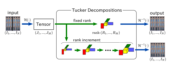
Figure 7: Illustration of the tensor completion using embedding transform.

5 Experiments

In this section, we conduct several experiments on color image $``$ peppers $"$ using different tensor completion methods, which include factorization based approaches and rank minimization based approaches. The sampling methods of all test experiments are random sampling with respect to different sampling ratios (SR), which is defined as:

$$\text{SR}=\frac{O}{\prod_{n=1}^{N}I_{n}}$$ (35)

where $O$ is the number of observation entries, $I_{n}$, $n=1,\dots,N$ is the dimension corresponding to mode $k$.

To measure the recovered performance of tensor completion algorithms, the relative error between the original tensor and recovered tensor, which is the most used evaluation metric, has been defined as:

$$\text{Rel}=\lVert\mathcal{\bar{X}}-\mathcal{X}\rVert_{\text{F}}/\lVert\mathcal{X}\rVert_{\text{F}},$$ (36)

where $\mathcal{\bar{X}}$ is the recovered tensor and $\mathcal{X}$ is the original tensor. Besides, peak signal-to-noise ratio (PSNR) and structural similarity index (SSIM) are the commonly applied in images recovery. The PSNR is the error between the original and reconstructed images, which is defined as:

$$\text{PSNR}=20\log_{10}(\operatorname{MAX}/\operatorname{\sqrt{MSE}}),$$ (37)

where $\operatorname{MAX}$ is the maximum value of all the pixels in the image, and mean squared error (MSE) is defined as:

$$\operatorname{MSE}=\lVert\mathcal{P}_{\mathbb{O}}\ast(\hat{\mathcal{X}}-\mathcal{X})\rVert_{\text{F}}^{2}/\lVert\mathcal{P}_{\mathbb{O}}\rVert_{\text{F}}^{2}.$$ (38)

The SSIM measures the similarity of two images based on three comparison measurements with respect to luminance, contrast and structure, which is defined as:

$$\operatorname{SSIM}=l(\mathcal{X},\mathcal{\hat{X}})^{\alpha}\cdot c(\mathcal{X},\mathcal{\hat{X}})^{\beta}\cdot s(\mathcal{X},\mathcal{\hat{X}})^{\gamma},$$ (39)

where $\alpha$, $\beta$ and $\gamma$ are the weights corresponding to the luminance measurement $l(\mathcal{X},\mathcal{\hat{X}})$, contrast measurement $c(\mathcal{X},\mathcal{\hat{X}})$, structure measurement $s(\mathcal{X},\mathcal{\hat{X}})$.

Fig. 8 shows the recovered images using ALS algorithms using different decomposition with a given bound rank. We set the bound ranks parameters as: $10$, $[10,10,3]$, $[1,10,10,1]$, $[10,10,10]$ for CP rank bound, tucker rank bound, tensor train rank bound and tensor ring rank bound, respectively.

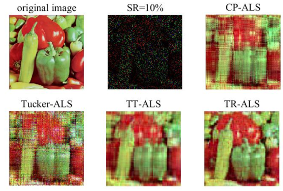
Figure 8: Recovered the peppers image using different methods with a given bound rank.

Fig. 9 shows the metric using Rel, PSNR and SSIM with SR from 10% to 40%. From the Fig. 9, we could observe that different decomposition methods with the same rank bound under the SR changes from 10% to 40%, the result is different.

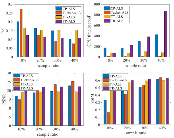
Figure 9: The performance of different decomposition method with a bound rank in terms of Rel, CPU time, PSNR and SSIM.

Fig. 10 are recovered results with different rank minimization under the $\text{SR}=20\%$. And Fig. 11 shows the performance of different rank minimization with respect to Rel, PSNR and SSIM under the SR changes from 10% to 40%.

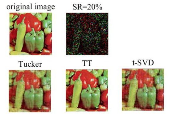
Figure 10: The recovered results with different rank minimization.

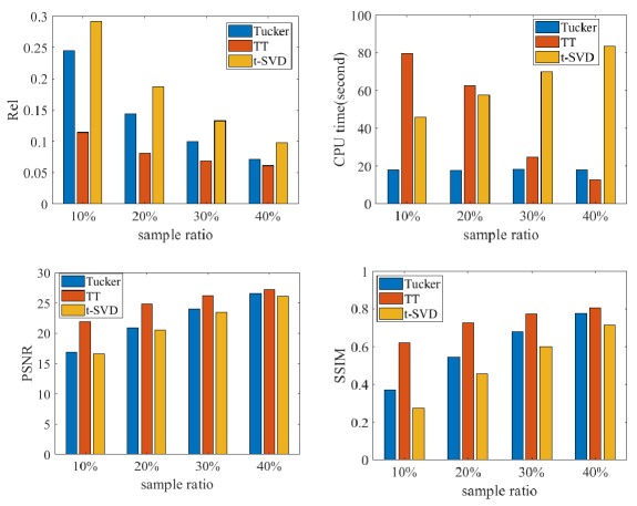
Figure 11: The performance of different decomposition method with rank minimization in terms of Rel, CPU time, PSNR and SSIM.

6 Conclusions

In this review, we provide clear guidelines of tensor completion for researchers in processing color images and videos. First, we divided tensor completion algorithms into two groups according to predefined rank and rank minimization, and then for each group, we introduce a variety of optimization models in details with respect to different tensor decomposition. Additionally, we conduct a group of experiments using the factorization based approaches and rank minimization models. And we find that the rank minimization models perform well in terms of the accuracy and cost time.

7 Discussion and Future Work

We introduce a variety of tensor completion methods based on different tensor decomposition. Traditional tensor decompositions, such as CP decomposition and TucIker decomposition, have been studied many times. The CP decomposition can reduce the storage complexity from $I^{D}$ to $IDS$ where $D$ is the dimension of a tensor, $I$ is the size corresponding to dimension and $S$ is the CP rank, but the minimization of tensor nuclear norm for CP rank is an NP-hard problem. Hence, the existing low CP rank tensor completion methods often iteratively update the factor matrices with a predefined rank. The Tucker decomposition can reduce the storage complexity from $I^{D}$ to $IDS+S^{D}$, where $D$ is the dimension of a tensor, $I$ is the size corresponding to dimension， and we assume $S_{1}=S_{2}=\dots=S_{N}=S$, $\operatorname{rank}_{\text{Tucker}}=(S_{1},S_{2},\dots,S_{N})$, which indicts that the storage complexity grows exponentially with the dimensional increasing. In addition, t-SVD is a good extending of matrix, but it only suits for 3rd-order tensor. The simple tensor network decomposition including tensor train decomposition and tensor ring decomposition has shown its performance with traditional tensor composition, but the related work is little.

With the increasing of the data size, the computation cost of traditional tensor decomposition such as Tucker decomposition and CP decomposition is more expensive. In contrast, tensor network decomposition can replace it. Besides, more efficient and fast algorithms need to be proposed to deal with the big data. Furthermore, applying the tensor space into a higher-order space is one of the important work in the future.

8 Acknowledgment

The authors would like to thank Jiani Liu, Jiayi Fang and Huyan Huang for the helpful discussions. This research is supported by National Natural Science Foundation of China (NSFC, No. 61602091, No. 61571102) and the Fundamental Research Funds for the Central Universities (No. ZYGX2016J199, No. ZYGX2014Z003).

References

• (1) Cichocki A, Mandic D, De Lathauwer L, et al. Tensor decompositions for signal processing applications: From two-way to multiway component analysis[J]. IEEE Signal Processing Magazine, 2015, 32(2): 145-163.
• (2) Du B, Zhang M, Zhang L, et al. PLTD: Patch-based low-rank tensor decomposition for hyperspectral images[J]. IEEE Transactions on Multimedia, 2017, 19(1): 67-79.
• (3) Cong F, Lin Q H, Kuang L D, et al. Tensor decomposition of EEG signals: a brief review[J]. Journal of neuroscience methods, 2015, 248: 59-69.
• (4) Yokota T, Zdunek R, Cichocki A, et al. Smooth nonnegative matrix and tensor factorizations for robust multi-way data analysis[J]. Signal Processing, 2015, 113: 234-249.
• (5) Wu Z, Wang Q, Jin J, et al. Structure tensor total variation-regularized weighted nuclear norm minimization for hyperspectral image mixed denoising[J]. Signal Processing, 2017, 131: 202-219.
• (6) Zhou M, Liu Y, Long Z, et al. Tensor rank learning in CP decomposition via convolutional neural network[J]. Signal Processing: Image Communication, 2018.
• (7) Madathil B, George S N. Twist tensor total variation regularized-reweighted nuclear norm based tensor completion for video missing area recovery[J]. Information Sciences, 2018, 423: 376-397.
• (8) Jiang T X, Huang T Z, Zhao X L, et al. Matrix factorization for low-rank tensor completion using framelet prior[J]. Information Sciences, 2018, 436: 403-417.
• (9) Ji T Y, Huang T Z, Zhao X L, et al. Tensor completion using total variation and low-rank matrix factorization[J]. Information Sciences, 2016, 326: 243-257.
• (10) Szalay S, Pfeffer M, Murg V, et al. Tensor product methods and entanglement optimization for ab initio quantum chemistry[J]. International Journal of Quantum Chemistry, 2015, 115(19): 1342-1391.
• (11) Khoromskaia V, Khoromskij B N. Tensor numerical methods in quantum chemistry: from Hartree–Fock to excitation energies[J]. Physical Chemistry Chemical Physics, 2015, 17(47): 31491-31509.
• (12) Schütt K T, Arbabzadah F, Chmiela S, et al. Quantum-chemical insights from deep tensor neural networks[J]. Nature communications, 2017, 8: 13890.
• (13) He Z, Hu J, Wang Y. Low-rank tensor learning for classification of hyperspectral image with limited labeled samples[J]. Signal Processing, 2018, 145: 12-25.
• (14) Guo H, Wu X, Feng W. Multi-stream deep networks for human action classification with sequential tensor decomposition[J]. Signal Processing, 2017, 140: 198-206.
• (15) Vigneron V, Kodewitz A, Da Costa M N, et al. Non-negative sub-tensor ensemble factorization (NsTEF) algorithm. A new incremental tensor factorization for large data sets[J]. Signal Processing, 2018, 144: 77-86.
• (16) Zheng Y. Trajectory data mining: an overview[J]. ACM Transactions on Intelligent Systems and Technology (TIST), 2015, 6(3): 29.
• (17) Papalexakis E E, Faloutsos C, Sidiropoulos N D. Tensors for data mining and data fusion: Models, applications, and scalable algorithms[J]. ACM Transactions on Intelligent Systems and Technology (TIST), 2017, 8(2): 16.
• (18) Sael L, Jeon I, Kang U. Scalable tensor mining[J]. Big Data Research, 2015, 2(2): 82-86.
• (19) Candès E J, Recht B. Exact matrix completion via convex optimization[J]. Foundations of Computational mathematics, 2009, 9(6): 717.
• (20) Cai J F, Candès E J, Shen Z. A singular value thresholding algorithm for matrix completion[J]. SIAM Journal on Optimization, 2010, 20(4): 1956-1982.
• (21) Candès E J, Tao T. The power of convex relaxation: Near-optimal matrix completion[J]. IEEE Transactions on Information Theory, 2010, 56(5): 2053-2080.
• (22) Keshavan R H, Montanari A, Oh S. Matrix completion from a few entries[J]. IEEE Transactions on Information Theory, 2010, 56(6): 2980-2998.
• (23) Recht B. A simpler approach to matrix completion[J]. Journal of Machine Learning Research, 2011, 12(Dec): 3413-3430.
• (24) Jain P, Netrapalli P, Sanghavi S. Low-rank matrix completion using alternating minimization[C]//Proceedings of the forty-fifth annual ACM symposium on Theory of computing. ACM, 2013: 665-674.
• (25) Ji H, Liu C, Shen Z, et al. Robust video denoising using low rank matrix completion[C]//Computer Vision and Pattern Recognition (CVPR), 2010 IEEE Conference on. IEEE, 2010: 1791-1798.
• (26) Fazel M. Matrix rank minimization with applications[D]. PhD thesis, Stanford University, 2002.
• (27) Hu Y, Zhang D, Ye J, et al. Fast and accurate matrix completion via truncated nuclear norm regularization[J]. IEEE Transactions on Pattern Analysis and Machine Intelligence, 2013, 35(9): 2117-2130.
• (28) Lin X, Wei G. Accelerated reweighted nuclear norm minimization algorithm for low rank matrix recovery[J]. Signal Processing, 2015, 114: 24-33.
• (29) Song Q, Ge H, Caverlee J, et al. Tensor Completion Algorithms in Big Data Analytics[J]. arXiv preprint arXiv:1711.10105, 2017.
• (30) Cichocki A. Tensor networks for big data analytics and large-scale optimization problems[J]. arXiv preprint arXiv:1407.3124, 2014.
• (31) Carroll J D, Chang J J. Analysis of individual differences in multidimensional scaling via an N-way generalization of “Eckart-Young” decomposition[J]. Psychometrika, 1970, 35(3): 283-319.
• (32) Kolda T G, Bader B W. Tensor decompositions and applications[J]. SIAM review, 2009, 51(3): 455-500.
• (33) De Lathauwer L, De Moor B, Vandewalle J. A multilinear singular value decomposition[J]. SIAM journal on Matrix Analysis and Applications, 2000, 21(4): 1253-1278.
• (34) Kroonenberg P M, De Leeuw J. Principal component analysis of three-mode data by means of alternating least squares algorithms[J]. Psychometrika, 1980, 45(1): 69-97.
• (35) Tucker L R. Some mathematical notes on three-mode factor analysis[J]. Psychometrika, 1966, 31(3): 279-311.
• (36) Oseledets I V. Tensor-train decomposition[J]. SIAM Journal on Scientific Computing, 2011, 33(5): 2295-2317.
• (37) Zhao Q, Zhou G, Xie S, et al. Tensor ring decomposition[J]. arXiv preprint arXiv:1606.05535, 2016.
• (38) Smolensky P. Tensor product variable binding and the representation of symbolic structures in connectionist systems[J]. Artificial intelligence, 1990, 46(1-2): 159-216.
• (39) Guichardet A. Symmetric Hilbert spaces and related topics: Infinitely divisible positive definite functions. Continuous products and tensor products. Gaussian and Poissonian stochastic processes[M]. Springer, 2006.
• (40) Kilmer M E, Braman K, Hao N, et al. Third-order tensors as operators on matrices: A theoretical and computational framework with applications in imaging[J]. SIAM Journal on Matrix Analysis and Applications, 2013, 34(1): 148-172.
• (41) Boyd S, Parikh N, Chu E, et al. Distributed optimization and statistical learning via the alternating direction method of multipliers[J]. Foundations and Trends® in Machine learning, 2011, 3(1): 1-122.
• (42) Leurgans S E, Ross R T, Abel R B. A decomposition for three-way arrays[J]. SIAM Journal on Matrix Analysis and Applications, 1993, 14(4): 1064-1083.
• (43) Tomasi G, Bro R. PARAFAC and missing values[J]. Chemometrics and Intelligent Laboratory Systems, 2005, 75(2): 163-180.
• (44) Acar E, Dunlavy D M, Kolda T G, et al. Scalable tensor factorizations for incomplete data[J]. Chemometrics and Intelligent Laboratory Systems, 2011, 106(1): 41-56.
• (45) Kressner D, Steinlechner M, Vandereycken B. Low-rank tensor completion by Riemannian optimization[J]. BIT Numerical Mathematics, 2014, 54(2): 447-468.
• (46) Zhao Q, Zhang L, Cichocki A. Bayesian CP factorization of incomplete tensors with automatic rank determination[J]. IEEE Transactions on Pattern Analysis and Machine Intelligence, 2015, 37(9): 1751-1763.
• (47) Yokota T, Zhao Q, Cichocki A. Smooth PARAFAC decomposition for tensor completion[J]. IEEE Transactions on Signal Processing, 2016, 64(20): 5423-5436.
• (48) Andersson C A, Bro R. Improving the speed of multi-way algorithms:: Part I. Tucker3[J]. Chemometrics and intelligent laboratory systems, 1998, 42(1-2): 93-103.
• (49) Kasai H, Mishra B. Low-rank tensor completion: a Riemannian manifold preconditioning approach[C]//International Conference on Machine Learning. 2016: 1012-1021.
• (50) Heidel G, Schulz V. A Riemannian trust-region method for low-rank tensor completion[J]. arXiv preprint arXiv:1703.10019, 2017.
• (51) Rauhut H, Schneider R, Stojanac Ž. Low rank tensor recovery via iterative hard thresholding[J]. Linear Algebra and its Applications, 2017, 523: 220-262.
• (52) Goulart J H M, Favier G. An iterative hard thresholding algorithm with improved convergence for low-rank tensor recovery[C]//Signal Processing Conference (EUSIPCO), 2015 23rd European. IEEE, 2015: 1701-1705.
• (53) Vannieuwenhoven N, Vandebril R, Meerbergen K. A new truncation strategy for the higher-order singular value decomposition[J]. SIAM Journal on Scientific Computing, 2012, 34(2): A1027-A1052.
• (54) da Silva A P, Comon P, de Almeida A L F. A finite algorithm to compute rank-1 tensor approximations[J]. IEEE Signal Processing Letters, 2016, 23(7): 959-963.
• (55) de Morais Goulart J H, Comon P. A novel non-iterative algorithm for low-multilinear-rank tensor approximation[C]//Signal Processing Conference (EUSIPCO), 2017 25th European. IEEE, 2017: 653-657.
• (56) Grasedyck L, Kluge M, Krämer S. Variants of alternating least squares tensor completion in the tensor train format[J]. SIAM Journal on Scientific Computing, 2015, 37(5): A2424-A2450.
• (57) Grippo L, Sciandrone M. On the convergence of the block nonlinear Gauss–Seidel method under convex constraints[J]. Operations research letters, 2000, 26(3): 127-136.
• (58) Steinlechner M. Riemannian optimization for high-dimensional tensor completion[J]. SIAM Journal on Scientific Computing, 2016, 38(5): S461-S484.
• (59) Wen Z, Yin W, Zhang Y. Solving a low-rank factorization model for matrix completion by a nonlinear successive over-relaxation algorithm[J]. Mathematical Programming Computation, 2012, 4(4): 333-361.
• (60) Tan H, Cheng B, Wang W, et al. Tensor completion via a multi-linear low-n-rank factorization model[J]. Neurocomputing, 2014, 133: 161-169.
• (61) Xu Y, Hao R, Yin W, et al. Parallel matrix factorization for low-rank tensor completion[J]. arXiv preprint arXiv:1312.1254, 2013.
• (62) Bengua J A, Phien H N, Tuan H D, et al. Efficient tensor completion for color image and video recovery: Low-rank tensor train[J]. IEEE Transactions on Image Processing, 2017, 26(5): 2466-2479.
• (63) Tseng P. Convergence of a block coordinate descent method for nondifferentiable minimization[J]. Journal of Optimization Theory and Applications, 2001, 109(3): 475-494.
• (64) Wang W, Aggarwal V, Aeron S. Efficient low rank tensor ring completion[J]. Rn, 2017, 1(r1): 1.
• (65) Liu X Y, Aeron S, Aggarwal V, et al. Low-tubal-rank tensor completion using alternating minimization[C]//Modeling and Simulation for Defense Systems and Applications XI. International Society for Optics and Photonics, 2016, 9848: 984809.
• (66) Wang Y, Yang J, Yin W, et al. A new alternating minimization algorithm for total variation image reconstruction[J]. SIAM Journal on Imaging Sciences, 2008, 1(3): 248-272.
• (67) Wang L, Xie K, Semong T, et al. Missing Data Recovery Based on Tensor-CUR Decomposition[J]. IEEE Access, 2018, 6: 532-544.
• (68) Girson J, Aeron S. Tensor completion via optimization on the product of matrix manifolds[C]//Computational Advances in Multi-Sensor Adaptive Processing (CAMSAP), 2015 IEEE 6th International Workshop on. IEEE, 2015: 177-180.
• (69) Fletcher R, Powell M J D. A rapidly convergent descent method for minimization[J]. The Computer Journal, 1963, 6(2): 163-168.
• (70) Gillis N, Glineur F. Low-rank matrix approximation with weights or missing data is NP-hard[J]. SIAM Journal on Matrix Analysis and Applications, 2011, 32(4): 1149-1165.
• (71) Recht B, Fazel M, Parrilo P A. Guaranteed minimum-rank solutions of linear matrix equations via nuclear norm minimization[J]. SIAM review, 2010, 52(3): 471-501.
• (72) Toh K C, Yun S. An accelerated proximal gradient algorithm for nuclear norm regularized linear least squares problems[J]. Pacific Journal of optimization, 2010, 6(615-640): 15.
• (73) Liu J, Musialski P, Wonka P, et al. Tensor completion for estimating missing values in visual data[J]. IEEE Transactions on Pattern Analysis and Machine Intelligence, 2013, 35(1): 208-220.
• (74) Gandy S, Recht B, Yamada I. Tensor completion and low-n-rank tensor recovery via convex optimization[J]. Inverse Problems, 2011, 27(2): 025010.
• (75) Xie J, Yang J, Tai Y, et al. Volume measurement based tensor completion[C]//Image Processing (ICIP), 2016 IEEE International Conference on. IEEE, 2016: 1838-1842.
• (76) Mu C, Huang B, Wright J, et al. Square deal: Lower bounds and improved relaxations for tensor recovery[C]//International Conference on Machine Learning. 2014: 73-81.
• (77) Romera-Paredes B, Pontil M. A new convex relaxation for tensor completion[C]//Advances in Neural Information Processing Systems. 2013: 2967-2975.
• (78) Liu Y, Shang F, Fan W, et al. Generalized higher order orthogonal iteration for tensor learning and decomposition[J]. IEEE Transactions on Neural Networks and Learning Systems, 2016, 27(12): 2551-2563.
• (79) Chen Y L, Hsu C T, Liao H Y M. Simultaneous tensor decomposition and completion using factor priors[J]. IEEE Transactions on Pattern Analysis and Machine Intelligence, 2014, 36(3): 577-591.
• (80) Yokota T, Hontani H. Simultaneous Visual Data Completion and Denoising Based on Tensor Rank and Total Variation Minimization and Its Primal-Dual Splitting Algorithm[C]//Proceedings of the IEEE Conference on Computer Vision and Pattern Recognition (CVPR). 2017: 3732-3740.
• (81) Yokota T, Hontani H. Simultaneous Tensor Completion and Denoising by Noise Inequality Constrained Convex Optimization[J]. arXiv preprint arXiv:1801.03299, 2018.
• (82) Bertsekas D P. Nonlinear programming[M]. Belmont: Athena scientific, 1999.
• (83) Zhang Z, Aeron S. Exact tensor completion using t-svd[J]. IEEE Transactions on Signal Processing, 2017, 65(6): 1511-1526.
• (84) Hu W, Tao D, Zhang W, et al. The twist tensor nuclear norm for video completion[J]. IEEE Transactions on Neural Networks and Learning Systems, 2017, 28(12): 2961-2973.
• (85) Zhang Z, Ely G, Aeron S, et al. Novel methods for multilinear data completion and de-noising based on tensor-SVD[C]//Proceedings of the IEEE Conference on Computer Vision and Pattern Recognition. 2014: 3842-3849.
• (86) Xue S, Qiu W, Liu F, et al. Low-Rank Tensor Completion by Truncated Nuclear Norm Regularization[J]. arXiv preprint arXiv:1712.00704, 2017.
• (87) George S N. Reweighted Low-Rank Tensor Completion and its Applications in Video Recovery[J]. arXiv preprint arXiv:1611.05964, 2016.
• (88) Yokota T, Erem B, Guler S, et al. Missing Slice Recovery for Tensors Using a Low-rank Model in Embedded Space[J]. arXiv preprint arXiv:1804.01736, 2018.