Lattice QCD study of the $H$ dibaryon using hexaquark and two-baryon interpolators

Abstract

We present a lattice QCD spectroscopy study in the isospin singlet, strangeness $-2$ sectors relevant for the conjectured $H$ dibaryon. We employ both local and bilocal interpolating operators to isolate the ground state in the rest frame and in moving frames. Calculations are performed using two flavors of $O(a)$-improved Wilson fermions and a quenched strange quark. Our initial point-source method for constructing correlators does not allow for bilocal operators at the source; nevertheless, results from using these operators at the sink indicate that they provide an improved overlap onto the ground state in comparison with the local operators. We also present results, in the rest frame, using a second method based on distillation to compute a hermitian matrix of correlators with bilocal operators at both the source and the sink. This method yields a much more precise and reliable determination of the ground-state energy. In the flavor-SU(3) symmetric case, we apply Lüscher’s finite-volume quantization condition to the rest-frame and moving-frame energy levels to determine the $S$-wave scattering phase shift, near and below the two-particle threshold. For a pion mass of 960 MeV, we find that there exists a bound $H$ dibaryon with binding energy ${\Delta}E=(19\pm 10)$ MeV. In the 27-plet (dineutron) sector, the finite-volume analysis suggests that the existence of a bound state is unlikely.

I Introduction

The strong force between quarks and gluons produces a rich spectrum of bound states and resonances, the color-neutral hadrons. Most of these can be described by constituent quark models as either quark-antiquark mesons or three-quark baryons. The existence of exotic hadrons, which cannot be described as such, is an active field of inquiry. Over the past several years, the so-called “X, Y, Z” mesons have been studied intensively, both theoretically and experimentally Lebed:2016hpi , and in recent years pentaquark baryons have also gained attention Aaij:2015tga .

Nearly four decades ago, using the MIT bag model, Jaffe predicted a deeply bound dibaryon with quark content $uuddss$ that is a scalar and a flavor singlet, the $H$ dibaryon Jaffe:1976yi . In contrast with the only known stable dibaryon, the deuteron, which can be well described as a loosely-bound proton-neutron state and is bound by just 2.2 MeV, the bag model predicted the $H$ dibaryon as an exotic hexaquark state where all six quarks are in S-wave in the same hadronic bag, bound by about 80 MeV below the $\Lambda\Lambda$ threshold.

Experimental evidence disfavors such a large binding energy. The strongest constraint is the “Nagara” event provided by the E373 experiment at KEK Takahashi:2001nm , which found a $\isotope[6][\Lambda\Lambda]{He}$ double-hypernucleus with $\Lambda\Lambda$ binding energy $B_{\Lambda\Lambda}=6.91\pm 0.16$ MeV Nakazawa:2010zza that decayed weakly. A deeply bound $H$ dibaryon would enable the strong decay $\isotope[6][\Lambda\Lambda]{He}\to\isotope[4]{He}+H$; its absence implies $m_{H}>2m_{\Lambda}-B_{\Lambda\Lambda}$. There was also no indication of an $H$ dibaryon from a high-statistics study of upsilon decays at Belle Kim:2013vym .

The first lattice QCD study of the $H$ dibaryon was performed more than thirty years ago Mackenzie:1985vv , using a quenched ensemble with lattice size $6^{2}\times 12\times 18$. Quenched studies — which all used local interpolating operators with six quarks at the same point in keeping with the bag model picture, together with standard lattice spectroscopy techniques — produced inconclusive results: while some found a bound state Iwasaki:1987db ; Luo:2007zzb ; Luo:2011ar , others did not Mackenzie:1985vv ; Pochinsky:1998zi ; Wetzorke:1999rt ; Wetzorke:2002mx . Early studies of the $H$ dibaryon using lattice QCD are summarized in Ref. Beane:2011zpa .

Aside from the present work, calculations with dynamical fermions have been performed by two collaborations, both of which reported a bound $H$ dibaryon at heavier-than-physical quark masses. The NPLQCD collaboration performed lattice spectroscopy calculations using a setup based on clover fermions with local hexaquark operators at the source and bilocal two-baryon operators at the sink. First results were obtained on anisotropic ensembles with $N_{f}=2+1$ dynamical fermions Beane:2010hg ; Beane:2011zpa ; Beane:2011iw , followed by isotropic ensembles with three mass-degenerate ($N_{f}=3$) quarks Beane:2012vq . An alternative approach, employed by the HAL QCD collaboration, is based on determining baryon-baryon potentials from Nambu-Bethe-Salpeter wave functions computed on the lattice, followed by solving the Schrödinger equation to study baryon-baryon scattering and bound states. This was done on ensembles with $N_{f}=3$ clover fermions for a range of quark masses Inoue:2010hs ; Inoue:2010es ; Inoue:2011ai . Although these two sets of calculations agreed on the presence of a bound state, they disagreed significantly on the binding energy: in the $N_{f}=3$ case with pseudoscalar meson mass near 800 MeV, the value reported by NPLQCD was $74.6\pm 4.7$ MeV, whereas HAL QCD reported $37.8\pm 5.1$ MeV. Recently, HAL QCD have published a $N_{f}=2+1$ study of coupled channel ($\Lambda\Lambda$ and $N\Xi$) baryon-baryon interactions with near-physical quark masses, which claims that the $H$ dibaryon may be a $\Lambda\Lambda$ resonance just below the $N\Xi$ threshold Sasaki:2016gpc ; Sasaki:2018mzh .

Given that there are conflicting results for the binding energy of the $H$ dibaryon, we have started a new initiative which may help to resolve the issue. As a first step we present results from a study in two-flavor QCD, i.e. with a mass-degenerate doublet of dynamical $u$ and $d$ quarks. The mass of the (quenched) strange quark is either tuned such that $m_{s}=m_{d}=m_{u}$ or set to a heavier value, implying that the SU(3) flavor symmetry is broken. Clearly, SU(3) symmetry is significantly broken at the physical point Haidenbauer:2011ah ; Haidenbauer:2011za , which allows the three flavor multiplets, i.e. the singlet, octet and 27-plet to couple. Therefore, it is advantageous to study the octet and 27-plet even in the case of exact SU(3) symmetry. Furthermore, the 27-plet contains the two-nucleon $I=1$ sector which has a possible dineutron bound state. The nucleon-nucleon sector has been studied extensively in experiment and may serve as a benchmark for lattice calculations.

Our work is mainly focused on the methodology of determining the spectrum and the binding energy via the computation of correlation matrices and their diagonalization Michael:1985ne ; Luscher:1990ck ; Blossier:2009kd . In order to allow for a direct comparison with the results from older quenched studies and from NPLQCD we have chosen a similar setup. As we will describe in more detail in the following sections, we have used point sources to compute correlator matrices with local interpolating operators at the source and both local and bilocal interpolators at the sink. In addition, we report initial results from a follow-up study in which we, for the first time, applied the distillation method Peardon:2009gh to the two-baryon sector. This allowed us to compute a correlator matrix using operators made from products of two spatially displaced, momentum-projected baryon interpolators at both the source and the sink. We shall see that this hermitian setup leads to a more robust and precise identification of the spectrum.

Since the strange quark is quenched in our calculation, one may think that any observed deviation from the findings of Refs. Beane:2010hg ; Beane:2011zpa ; Beane:2011iw ; Beane:2012vq ; Inoue:2010hs ; Inoue:2010es ; Inoue:2011ai should be attributed to the different treatment of the quark sea. However, the FLAG report Aoki:2016frl provides ample evidence that observables computed with $N_{\text{f}}=2$ or $N_{\text{f}}=2+1$ dynamical quarks differ at the percent level at most.

This paper is organized as follows. Our methodology is described in Section II: this includes the interpolating operators and our approach for analyzing correlator matrices. We show our determination of the energy levels using point-source methods in Section III.1 and using distillation in Section III.2. In Section IV, we apply Lüscher’s finite-volume quantization condition to determine scattering phase shifts at the SU(3)-symmetric point, and identify the presence of a bound $H$ dibaryon. Finally, our conclusions are presented in Section V.

II Lattice calculation and setup

II.1 Simulation details

Our study has been performed on a set of ensembles with two mass-degenerate dynamical flavors of O($a$)-improved Wilson quarks Sheikholeslami:1985ij and the Wilson plaquette action, which were generated as part of the CLS (Coordinated Lattice Simulations) initiative, using the deflation-accelerated DD-HMC Luscher:2005rx ; Luscher:2007es and MP-HMC Marinkovic:2010eg algorithms. The improvement coefficient $c_{\rm sw}$ multiplying the Sheikholeslami-Wohlert term was tuned according to the non-perturbative determination of Ref. Jansen:1998mx . An overview of the ensembles can be found in Table 1. All our calculations were performed in the SU(3)-flavor symmetric limit, with the exception of ensemble E5 for which the valence strange quark mass was tuned so that the combination $(2m_{K}^{2}-m_{\pi}^{2})/m_{\Omega}^{2}$ takes its physical value. The corresponding values of $m_{\pi}$ and $m_{K}$ are provided in the table. The values of the lattice spacing in physical units were determined using the kaon decay constant Fritzsch:2012wq .

Quark propagators were computed using the Schwarz alternating procedure (SAP) domain-decomposed, deflated generalized conjugate residual (GCR) solver of the DD-HMC package Luscher:2005rx with smeared point sources on a grid of source positions that was randomly displaced on each gauge configuration. For the distillation calculation, we used a similar solver in OpenQCD OpenQCD , computed low modes of the spatial Laplacian using PRIMME PRIMME , and contracted them to form “perambulators” and mode triplets using QDP++ Edwards:2004sx . Baryon and multi-baryon correlators computed in lattice QCD suffer from a severe signal-to-noise problem, since the noise grows with a rate proportional to $\exp\{({m_{\rm B}-3/2m_{\pi})t}\}$ per baryon, where $m_{\rm B}$ denotes the baryon mass. This makes it difficult to identify a “window” in which the asymptotic behavior has been reached while the signal is not yet lost in the statistical noise. In order to allow for a significant increase in statistics while keeping the numerical effort at a manageable level, we have employed the method of all-mode-averaging (AMA) Blum:2012uh . This entails computing a high number of samples with lower-precision propagator solves, followed by applying a bias correction using a relatively small number of high-precision solves. We used this for the calculation with point-source propagators, but obtained only modest cost savings due to our use of a highly efficient solver.

	point-to-all				timeslice-to-all
Label	N1	E5	E1	A1	E5	E1
Size	$\>48^{3}\times 96\>$	$\>32^{3}\times 64\>$	$\>32^{3}\times 64\>$	$\>32^{3}\times 64\>$	$\>32^{3}\times 64\>$	$\>32^{3}\times 64\>$
$\beta$	5.5	5.3	5.3	5.2	5.3	5.3
$a\;\left[\text{fm}\right]$	0.0486(6)	0.0658(10)	0.0658(10)	0.0755(11)	0.0658(10)	0.0658(10)
$m_{\pi}\;\left[\text{MeV}\right]$	858	436	960	744	436	960
$m_{K}\;\left[\text{MeV}\right]$	858	648	960	744	648	960
$L\;\left[\text{fm}\right]$	2.33	2.11	2.11	2.42	2.11	2.11
$m_{\pi}L$	10.0	4.7	10.2	9.9	4.7	10.2
$N_{\text{conf}}$	100	1990	168	286	2000	168
$N_{\text{src}}|N_{\text{tsrc}}$	128	32	128	128	4	8
$N_{\text{meas}}$	25600	127360	43008	73216	16000	2688

Table 1: Overview of ensemble parameters used in this study. For ensembles N1, E1 and A1 all quark masses were tuned to realize the SU(3)-flavor symmetric case, while for E5 the quark masses are non-degenerate. $N_{\text{src}}$ denotes the number of sources in the calculation of point-to-all propagators using the AMA method, while $N_{\text{tsrc}}$ is the number of timeslices used to compute timeslice-to-all propagators with the distillation method. For every configuration and source position we have computed the correlators in the forward and backward directions, resulting in two independent measurements.

II.2 Interpolating operators

Accurate determinations of the spectrum in the $H$ dibaryon channel require a set of efficient interpolating operators whose projection properties onto the ground state may also give qualitative insights into the nature of the $H$ dibaryon. For instance, the local operators defined in Equation (2) below resemble more closely Jaffe’s original interpretation of the $H$ dibaryon as a deeply bound state of six quarks forming a color singlet. By contrast, bilocal two-baryon operators (see Equation (6)) may be more appropriate to describe loosely-bound states such as the deuteron. While the two types of operators are defined according to a qualitative physical picture that is suggestive of the nature of a given state, this is not a rigorous way to study its properties.

The generic form of a lattice QCD correlation function is given by

$$C_{ij}(\mathchoice{\mbox{\boldmath$\displaystyle P$}}{\mbox{\boldmath$\textstyle P$}}{\mbox{\boldmath$\scriptstyle P$}}{\mbox{\boldmath$\scriptscriptstyle P$}},\tau)=\left\langle\mathcal{O}_{i}({\mathchoice{\mbox{\boldmath$\displaystyle P$}}{\mbox{\boldmath$\textstyle P$}}{\mbox{\boldmath$\scriptstyle P$}}{\mbox{\boldmath$\scriptscriptstyle P$}}},t)\mathcal{O}_{j}({\mathchoice{\mbox{\boldmath$\displaystyle P$}}{\mbox{\boldmath$\textstyle P$}}{\mbox{\boldmath$\scriptstyle P$}}{\mbox{\boldmath$\scriptscriptstyle P$}}},t^{\prime})^{\dagger}\right\rangle,\quad\tau=t-t^{\prime},$$ (1)

where the interpolating operator $\mathcal{O}_{i}$ carries the quantum numbers of the continuum state under study, and it is understood that $\mathcal{O}_{i}$ has been projected onto spatial momentum $\textstyle P$. When constructing interpolators in the $H$ dibaryon channel, one can think of two generic configurations. Jaffe’s original analysis was based on a compact color-singlet comprising six quarks, which gives rise to a hexaquark operator composed of flavors $uuddss$. The alternative possibility is the product of two individual color-singlets at different positions, i.e. a two-baryon operator.

The starting point for the construction of local hexaquark operators is the object

$$[rstuvw]=\epsilon_{ijk} \epsilon_{lmn}\Big{(}s^{i}C\gamma_{5}P_{+}t^{j}\Big{)}$$ (2)

$$\times\Big{(}v^{l}C\gamma_{5}P_{+}w^{m}\Big{)}\Big{(}r^{k}C\gamma_{5}P_{+}u^{n}\Big{)}({\mathchoice{\mbox{\boldmath$\displaystyle x$}}{\mbox{\boldmath$\textstyle x$}}{\mbox{\boldmath$\scriptstyle x$}}{\mbox{\boldmath$\scriptscriptstyle x$}}},t)\,,$$

where $r,s,\ldots,w$ denote generic quark flavors, and $P_{+}=(1+\gamma_{0})/2$ projects the quark fields to positive parity. One can form two operators that transform under the singlet Donoghue:1986zd ; Golowich:1992zw ; Wetzorke:1999rt and 27-plet irreducible representations of flavor SU(3):

$$H_{\mathbf{1}} =\frac{1}{48}\Big{(}[sudsud]-[udusds]-[dudsus]\Big{)},$$ (3)

$$H_{\mathbf{27}} =\frac{1}{48\sqrt{3}}\Big{(}3[sudsud]+[udusds]+[dudsus]\Big{)}\,.$$ (4)

The continuum quantum numbers of these operators are $S=-2$, $I(J^{P})=0(0^{+})$, as required by the original bag-model proposal. Equation (2) is the product of two single-baryon operators with quark content $rst$ and $uvw$ at the same point; one could then interpret $H_{\mathbf{1}}$ and $H_{\mathbf{27}}$ as linear combinations of $\Lambda\Lambda$ and $p\Xi^{-}+n\Xi^{0}$. However, as argued in Ref. Golowich:1992zw , this is not meaningful because antisymmetrization of the six quarks implies that the operators are also equal to linear combinations of $\Lambda\Lambda$ and $\Sigma\Sigma$. Similarly, $H_{\mathbf{1}}$ could also be written as the product of two color-octet triquarks Donoghue:1986zd or of three diquarks Jaffe:2004ph . We stress that it is the unique SU(3)-singlet scalar operator made from six positive-parity-projected quarks at the same point. We also note that an octet state cannot be represented in terms of this simplest class of hexaquark operators. Finally, we project onto the momentum of each lattice frame:

$$H_{\{\mathbf{1,27}\}}(\mathchoice{\mbox{\boldmath$\displaystyle P$}}{\mbox{\boldmath$\textstyle P$}}{\mbox{\boldmath$\scriptstyle P$}}{\mbox{\boldmath$\scriptscriptstyle P$}},t)=\sum_{\mathchoice{\mbox{\boldmath$\displaystyle x$}}{\mbox{\boldmath$\textstyle x$}}{\mbox{\boldmath$\scriptstyle x$}}{\mbox{\boldmath$\scriptscriptstyle x$}}}e^{-i\mathchoice{\mbox{\boldmath$\displaystyle P\cdot x$}}{\mbox{\boldmath$\textstyle P\cdot x$}}{\mbox{\boldmath$\scriptstyle P\cdot x$}}{\mbox{\boldmath$\scriptscriptstyle P\cdot x$}}}H_{\{\mathbf{1,27}\}}(\mathchoice{\mbox{\boldmath$\displaystyle x$}}{\mbox{\boldmath$\textstyle x$}}{\mbox{\boldmath$\scriptstyle x$}}{\mbox{\boldmath$\scriptscriptstyle x$}},t).$$ (5)

From now on, we will refer to this type of interpolator as a local hexaquark operator.

An alternative configuration in the $H$ dibaryon channel is described by the product of two spatially displaced, momentum-projected single baryon operators Inoue:2010hs :

$$\big{(}BB\big{)}_{m}({\mathchoice{\mbox{\boldmath$\displaystyle P$}}{\mbox{\boldmath$\textstyle P$}}{\mbox{\boldmath$\scriptstyle P$}}{\mbox{\boldmath$\scriptscriptstyle P$}}},t)=\sum_{\mathchoice{\mbox{\boldmath$\displaystyle p_{1}$}}{\mbox{\boldmath$\textstyle p_{1}$}}{\mbox{\boldmath$\scriptstyle p_{1}$}}{\mbox{\boldmath$\scriptscriptstyle p_{1}$}},\mathchoice{\mbox{\boldmath$\displaystyle p_{2}$}}{\mbox{\boldmath$\textstyle p_{2}$}}{\mbox{\boldmath$\scriptstyle p_{2}$}}{\mbox{\boldmath$\scriptscriptstyle p_{2}$}}}f_{m}(\mathchoice{\mbox{\boldmath$\displaystyle p_{1}$}}{\mbox{\boldmath$\textstyle p_{1}$}}{\mbox{\boldmath$\scriptstyle p_{1}$}}{\mbox{\boldmath$\scriptscriptstyle p_{1}$}},\mathchoice{\mbox{\boldmath$\displaystyle p_{2}$}}{\mbox{\boldmath$\textstyle p_{2}$}}{\mbox{\boldmath$\scriptstyle p_{2}$}}{\mbox{\boldmath$\scriptscriptstyle p_{2}$}})$$ (6)

$$\times\sum_{{\mathchoice{\mbox{\boldmath$\displaystyle x$}}{\mbox{\boldmath$\textstyle x$}}{\mbox{\boldmath$\scriptstyle x$}}{\mbox{\boldmath$\scriptscriptstyle x$}}}}e^{-i{\mathchoice{\mbox{\boldmath$\displaystyle p_{1}\cdot x$}}{\mbox{\boldmath$\textstyle p_{1}\cdot x$}}{\mbox{\boldmath$\scriptstyle p_{1}\cdot x$}}{\mbox{\boldmath$\scriptscriptstyle p_{1}\cdot x$}}}}B_{1\alpha}({\mathchoice{\mbox{\boldmath$\displaystyle x$}}{\mbox{\boldmath$\textstyle x$}}{\mbox{\boldmath$\scriptstyle x$}}{\mbox{\boldmath$\scriptscriptstyle x$}}},t)(C\gamma_{5}P_{+})_{\alpha\beta}\sum_{{\mathchoice{\mbox{\boldmath$\displaystyle y$}}{\mbox{\boldmath$\textstyle y$}}{\mbox{\boldmath$\scriptstyle y$}}{\mbox{\boldmath$\scriptscriptstyle y$}}}}e^{-i{\mathchoice{\mbox{\boldmath$\displaystyle p_{2}\cdot y$}}{\mbox{\boldmath$\textstyle p_{2}\cdot y$}}{\mbox{\boldmath$\scriptstyle p_{2}\cdot y$}}{\mbox{\boldmath$\scriptscriptstyle p_{2}\cdot y$}}}}B_{2\beta}({\mathchoice{\mbox{\boldmath$\displaystyle y$}}{\mbox{\boldmath$\textstyle y$}}{\mbox{\boldmath$\scriptstyle y$}}{\mbox{\boldmath$\scriptscriptstyle y$}}},t)\,,$$

where

$$B_{\alpha}=[rst]_{\alpha}=\epsilon_{ijk}\big{(}s^{i}C\gamma_{5}P_{+}t^{j}\big{)}r^{k}_{\alpha}\,,$$ (7)

and the individual baryons have been projected onto spatial momenta $\mathchoice{\mbox{\boldmath$\displaystyle p$}}{\mbox{\boldmath$\textstyle p$}}{\mbox{\boldmath$\scriptstyle p$}}{\mbox{\boldmath$\scriptscriptstyle p$}}_{1}$ and $\mathchoice{\mbox{\boldmath$\displaystyle p$}}{\mbox{\boldmath$\textstyle p$}}{\mbox{\boldmath$\scriptstyle p$}}{\mbox{\boldmath$\scriptscriptstyle p$}}_{2}$ with total momentum $\mathchoice{\mbox{\boldmath$\displaystyle P$}}{\mbox{\boldmath$\textstyle P$}}{\mbox{\boldmath$\scriptstyle P$}}{\mbox{\boldmath$\scriptscriptstyle P$}}=\mathchoice{\mbox{\boldmath$\displaystyle p$}}{\mbox{\boldmath$\textstyle p$}}{\mbox{\boldmath$\scriptstyle p$}}{\mbox{\boldmath$\scriptscriptstyle p$}}_{1}+\mathchoice{\mbox{\boldmath$\displaystyle p$}}{\mbox{\boldmath$\textstyle p$}}{\mbox{\boldmath$\scriptstyle p$}}{\mbox{\boldmath$\scriptscriptstyle p$}}_{2}$. The index $m$ labels a particular configuration of momenta $\mathchoice{\mbox{\boldmath$\displaystyle p$}}{\mbox{\boldmath$\textstyle p$}}{\mbox{\boldmath$\scriptstyle p$}}{\mbox{\boldmath$\scriptscriptstyle p$}}_{1}$ and $\mathchoice{\mbox{\boldmath$\displaystyle p$}}{\mbox{\boldmath$\textstyle p$}}{\mbox{\boldmath$\scriptstyle p$}}{\mbox{\boldmath$\scriptscriptstyle p$}}_{2}$. In the rest frame, the momentum combinations have a particularly simple construction:

$$f_{m}(\mathchoice{\mbox{\boldmath$\displaystyle p$}}{\mbox{\boldmath$\textstyle p$}}{\mbox{\boldmath$\scriptstyle p$}}{\mbox{\boldmath$\scriptscriptstyle p$}}_{1},\mathchoice{\mbox{\boldmath$\displaystyle p$}}{\mbox{\boldmath$\textstyle p$}}{\mbox{\boldmath$\scriptstyle p$}}{\mbox{\boldmath$\scriptscriptstyle p$}}_{2})=\begin{cases}1&\mathchoice{\mbox{\boldmath$\displaystyle p$}}{\mbox{\boldmath$\textstyle p$}}{\mbox{\boldmath$\scriptstyle p$}}{\mbox{\boldmath$\scriptscriptstyle p$}}_{1}=-\mathchoice{\mbox{\boldmath$\displaystyle p$}}{\mbox{\boldmath$\textstyle p$}}{\mbox{\boldmath$\scriptstyle p$}}{\mbox{\boldmath$\scriptscriptstyle p$}}_{2}\text{ and }\mathchoice{\mbox{\boldmath$\displaystyle p$}}{\mbox{\boldmath$\textstyle p$}}{\mbox{\boldmath$\scriptstyle p$}}{\mbox{\boldmath$\scriptscriptstyle p$}}_{1}^{2}=m\left({2\pi}/{L}\right)^{2}\\ 0&\text{otherwise}\end{cases}.$$ (8)

In the remainder of this paper, we refer to the object defined in Equation (6) as a bilocal two-baryon operator.

We form dibaryon operators from combinations of octet baryons with $S=-2$, $I=0$, i.e.

$$\big{(}\Lambda\Lambda\big{)} =\frac{1}{12}[sud][sud]~{}~{},$$ (9)

$$\begin{split}\big{(}N\Xi\big{)}_{S}&=\frac{1}{36}\Big{(}[uud][ssd]-[dud][ssu]\\ &\qquad+[ssd][uud]-[ssu][dud]\Big{)}~{}~{},\end{split}$$ (10)

$$\begin{split}\big{(}\Sigma\Sigma\big{)}&=\frac{1}{36\sqrt{3}}\Big{(}2[uus][dds]-[dus][uds]\\ &\qquad-[dus][dus]-[uds][dus]\\ &\qquad-[uds][uds]+2[dds][uus]\Big{)}~{},\end{split}$$ (11)

where the subscript $S$ on $(N\Xi)$ denotes the flavor-symmetric combination.

Using the rotation matrices listed in Appendix B of Ref. Inoue:2010hs we form the appropriate linear combinations of $(\Lambda\Lambda)$, $(N\Xi)_{S}$ and $(\Sigma\Sigma)$ that correspond to different flavor multiplets, i.e. the singlet, octet and 27-plet. The projected operators are then called $BB_{\{\mathbf{1,8,27}\},m}$.

In the interpolating operators defined above, we use smeared quark fields; the smearing helps to increase the coupling of an operator to the low-lying states. For the point-source calculation, we used Wuppertal smearing Gusken:1989qx , with the hopping term constructed using spatially APE-smeared Albanese:1987ds gauge links. To increase the size of our operator basis, we used two different smearing widths: “narrow” (70 steps, denoted $N$) and “medium” (140 steps, denoted $M$). The distillation approach makes use of Laplacian-Heaviside (LapH) smearing Peardon:2009gh , in which the quark fields are smeared by projecting them onto the low-lying modes of the spatial gauge-covariant Laplacian, itself constructed using stout-smeared Morningstar:2003gk gauge links. We used 56 modes in all cases, and label this type of smearing as $L$. We include the smearing as part of the label for each interpolating operator, yielding names such as $H_{\mathbf{1},N}$ or $BB_{\mathbf{27},L,0}$.

II.3 Operator basis and correlation matrices

The determination of hadronic energy levels in lattice QCD usually proceeds by computing a correlation matrix $C_{ij}(t)$ for the chosen basis of interpolating operators [see Equation (1)] and solving a generalized eigenvalue problem (GEVP) Michael:1985ne ; Luscher:1990ck ; Blossier:2009kd .

In the following the correlation matrices $C_{ij}(t)=C_{ij}(t,{\mathchoice{\mbox{\boldmath$\displaystyle P$}}{\mbox{\boldmath$\textstyle P$}}{\mbox{\boldmath$\scriptstyle P$}}{\mbox{\boldmath$\scriptscriptstyle P$}}})$ are evaluated at rest, i.e.  with total momentum ${\mathchoice{\mbox{\boldmath$\displaystyle P$}}{\mbox{\boldmath$\textstyle P$}}{\mbox{\boldmath$\scriptstyle P$}}{\mbox{\boldmath$\scriptscriptstyle P$}}}=0$, and in moving frames, i.e. ${\mathchoice{\mbox{\boldmath$\displaystyle P$}}{\mbox{\boldmath$\textstyle P$}}{\mbox{\boldmath$\scriptstyle P$}}{\mbox{\boldmath$\scriptscriptstyle P$}}}^{2}>0$. We included two-baryon operators with individual momenta $\mathchoice{\mbox{\boldmath$\displaystyle p$}}{\mbox{\boldmath$\textstyle p$}}{\mbox{\boldmath$\scriptstyle p$}}{\mbox{\boldmath$\scriptscriptstyle p$}}_{1,2}=2\pi\mathchoice{\mbox{\boldmath$\displaystyle d$}}{\mbox{\boldmath$\textstyle d$}}{\mbox{\boldmath$\scriptstyle d$}}{\mbox{\boldmath$\scriptscriptstyle d$}}_{1,2}/L$ and $\mathchoice{\mbox{\boldmath$\displaystyle d$}}{\mbox{\boldmath$\textstyle d$}}{\mbox{\boldmath$\scriptstyle d$}}{\mbox{\boldmath$\scriptscriptstyle d$}}^{2}=0,1,2,3$ in the calculation. The components were chosen such as to realize a total momentum $\mathchoice{\mbox{\boldmath$\displaystyle P$}}{\mbox{\boldmath$\textstyle P$}}{\mbox{\boldmath$\scriptstyle P$}}{\mbox{\boldmath$\scriptscriptstyle P$}}=\mathchoice{\mbox{\boldmath$\displaystyle p$}}{\mbox{\boldmath$\textstyle p$}}{\mbox{\boldmath$\scriptstyle p$}}{\mbox{\boldmath$\scriptscriptstyle p$}}_{1}+\mathchoice{\mbox{\boldmath$\displaystyle p$}}{\mbox{\boldmath$\textstyle p$}}{\mbox{\boldmath$\scriptstyle p$}}{\mbox{\boldmath$\scriptscriptstyle p$}}_{2}\equiv 2\pi\mathchoice{\mbox{\boldmath$\displaystyle D$}}{\mbox{\boldmath$\textstyle D$}}{\mbox{\boldmath$\scriptstyle D$}}{\mbox{\boldmath$\scriptscriptstyle D$}}/L$ with $\mathchoice{\mbox{\boldmath$\displaystyle D$}}{\mbox{\boldmath$\textstyle D$}}{\mbox{\boldmath$\scriptstyle D$}}{\mbox{\boldmath$\scriptscriptstyle D$}}^{2}=0,1,2,3$. For each $\mathchoice{\mbox{\boldmath$\displaystyle D$}}{\mbox{\boldmath$\textstyle D$}}{\mbox{\boldmath$\scriptstyle D$}}{\mbox{\boldmath$\scriptscriptstyle D$}}^{2}$, we average over all equivalent frames that are related by a lattice rotation.

$\langle H(t)H^{\dagger}(0)\rangle$                                         $\langle BB(t)H^{\dagger}(0)\rangle$

Figure 1: Quark lines for correlators using point sources. The vertical lines indicate that either the single or the two different end points of the quark lines are summed over the sink timeslice.

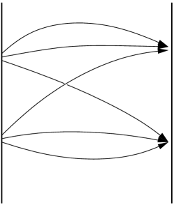
$\langle BB(t)BB^{\dagger}(0)\rangle$

Figure 2: Quark lines showing an example contraction for correlators using distillation. The vertical lines indicate that the two start and two end points for the quark lines are summed over the source and sink timeslice, respectively.

Performing the Wick contractions of correlators involving bilocal two-baryon operators of the type in Eq. (6) results in diagrams that contain quark lines that start or end at two distinct spatial points within a timeslice, This has important consequences for computing correlation matrices, since point-to-all propagators do not allow for the computation of such diagrams whenever a two-baryon operator is placed at the source. We therefore opted for an asymmetric setup in which only hexaquark operators were put at the source, while at the sink both hexaquark and two-baryon operators were used; this is illustrated in Figure 1. In this setting, the familiar GEVP or, more generally, the diagonalization procedure must be modified in order to allow for a non-hermitian correlator matrix. We select subsets of $N_{\textrm{op}}$ source operators and $N_{\textrm{op}}$ sink operators and form the corresponding square correlator matrix $\mathbf{C}(t)$. We then perform the following steps, starting from this $N_{\textrm{op}}\times N_{\textrm{op}}$ matrix:

1. Determine the right and left eigenvectors of $\mathbf{C}(t)$ by solving

   $$\mathbf{C}(t_{1})v_{n}(t_{1},t_{0}) =\lambda_{n}(t_{1},t_{0})\,\mathbf{C}(t_{0})v_{n}(t_{1},t_{0}),$$ (12)

   $$w_{n}^{\dagger}(t_{1},t_{0})\mathbf{C}(t_{1}) =\lambda_{n}(t_{1},t_{0})\,w_{n}^{\dagger}(t_{1},t_{0})\mathbf{C}(t_{0}),$$ (13)

   for $n=1,\ldots,N_{\textrm{op}}$, where $t_{0}$ and $t_{1}$ denote fixed timeslices in the region where the lowest $N_{\textrm{op}}$ states are expected to dominate.

2. Compute the (approximately) diagonal matrix $\mathbf{\Lambda}(t)$ whose elements are given by

   $$\Lambda_{nm}(t)=w_{n}^{\dagger}\mathbf{C}(t)v_{m}.$$ (14)

3. The effective $n$th energy level is then obtained from the diagonal element $\Lambda_{nn}(t)$ via the well-known formula

   $$E_{n}^{\rm eff}(t)=\frac{1}{{\Delta}t}\ln\frac{\Lambda_{nn}(t)}{\Lambda_{nn}(t+{\Delta}t)}.$$ (15)

We have used a timestep of ${\Delta}t=3a$ in our analysis. While the choice of interpolators at the source is restricted to hexaquark operators, we can probe a number of different operators at the sink and study their relevance for determining the ground state.

Relying on non-hermitian correlator matrices makes it more difficult to identify the ground state reliably, owing to the fact that the diagonalization does not project exactly on the correlator corresponding to the $n$th energy eigenstate. It is then not guaranteed that the effective energies computed via Eq. (15) approach the asymptotic value monotonically from above, since the statistical weights of different states are not strictly positive.

In order to overcome this difficulty we have implemented distillation and LapH smearing Peardon:2009gh . Since this is a timeslice-to-all rather than point-to-all method (see Figure 2), it allows us to compute a hermitian correlator matrix using the two-baryon operators listed in Eqs. (9)–(11), both in the center-of-mass frame and for non-vanishing total momentum $\textstyle P$. The main objects that we compute are the perambulator, which is the projection of the quark propagator onto the low modes of the spatial Laplacian, and the mode triplets,

$$T_{lnm}(t,\mathchoice{\mbox{\boldmath$\displaystyle p$}}{\mbox{\boldmath$\textstyle p$}}{\mbox{\boldmath$\scriptstyle p$}}{\mbox{\boldmath$\scriptscriptstyle p$}})=\sum_{\mathchoice{\mbox{\boldmath$\displaystyle x$}}{\mbox{\boldmath$\textstyle x$}}{\mbox{\boldmath$\scriptstyle x$}}{\mbox{\boldmath$\scriptscriptstyle x$}}}e^{-i\mathchoice{\mbox{\boldmath$\displaystyle p\cdot x$}}{\mbox{\boldmath$\textstyle p\cdot x$}}{\mbox{\boldmath$\scriptstyle p\cdot x$}}{\mbox{\boldmath$\scriptscriptstyle p\cdot x$}}}\epsilon_{ijk}u^{(l,t)}_{i}(\mathchoice{\mbox{\boldmath$\displaystyle x$}}{\mbox{\boldmath$\textstyle x$}}{\mbox{\boldmath$\scriptstyle x$}}{\mbox{\boldmath$\scriptscriptstyle x$}})u^{(n,t)}_{j}(\mathchoice{\mbox{\boldmath$\displaystyle x$}}{\mbox{\boldmath$\textstyle x$}}{\mbox{\boldmath$\scriptstyle x$}}{\mbox{\boldmath$\scriptscriptstyle x$}})u^{(m,t)}_{k}(\mathchoice{\mbox{\boldmath$\displaystyle x$}}{\mbox{\boldmath$\textstyle x$}}{\mbox{\boldmath$\scriptstyle x$}}{\mbox{\boldmath$\scriptscriptstyle x$}}),$$ (16)

where $u^{(l,t)}$ is the $l$th low mode on timeslice $t$. The correlator matrix is then computed by contracting these two objects. Further details of our implementation will appear in future work; here we present initial results in the rest frame using operators with both baryons at rest, i.e. $\mathchoice{\mbox{\boldmath$\displaystyle p$}}{\mbox{\boldmath$\textstyle p$}}{\mbox{\boldmath$\scriptstyle p$}}{\mbox{\boldmath$\scriptscriptstyle p$}}_{1}=\mathchoice{\mbox{\boldmath$\displaystyle p$}}{\mbox{\boldmath$\textstyle p$}}{\mbox{\boldmath$\scriptstyle p$}}{\mbox{\boldmath$\scriptscriptstyle p$}}_{2}=\mathchoice{\mbox{\boldmath$\displaystyle 0$}}{\mbox{\boldmath$\textstyle 0$}}{\mbox{\boldmath$\scriptstyle 0$}}{\mbox{\boldmath$\scriptscriptstyle 0$}}$. For a hermitian correlator matrix, the right and left eigenvectors are obviously identical.

In the case of broken SU(3) symmetry, the diagonalization method also allows us to associate a state with a particular multiplet, by identifying which operators couple most strongly to it. Furthermore, an essential feature of this method — as will be shown in Section III.1.2 — is that it can identify the presence of more than one state, even when the statistical signal is too poor to distinguish the energies of those states.

We end this section with a remark on SU(3) flavor symmetry in our setup, in which the strange quark is not present in the sea. In this case flavor symmetry is realized by the graded group SU$(3|1)$. SU(3) is a subgroup of SU$(3|1)$, and the flavor symmetry of our operator construction is exact, even at the level of individual gauge configurations. We have verified this by computing off-diagonal correlators between different multiplets and found them to vanish within errors.

III Energy levels

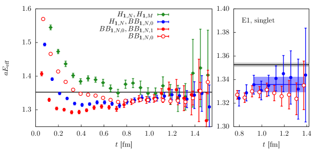
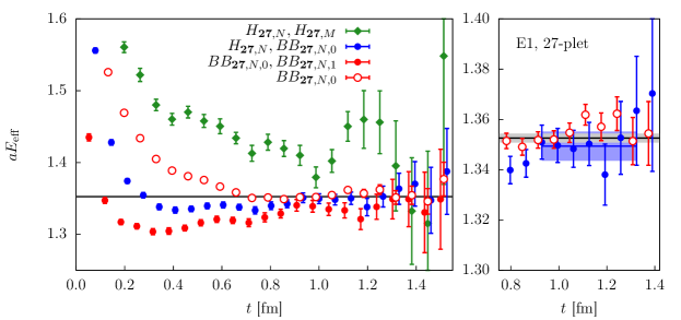
Figure 3: Ground-state effective energy for the singlet (top) and 27-plet (bottom) on ensemble E1. The legend indicates the operators used at the sink. Solid green diamonds denote the energies determined from the hermitian $2\times 2$ GEVP, while the solid blue and red circles represent the results extracted from the non-hermitian $2\times 2$ matrix. Open red circles correspond to the effective energy obtained from a single correlation function with a narrow-smeared hexaquark operator at the source and a two-baryon operator with $\mathchoice{\mbox{\boldmath$\displaystyle p$}}{\mbox{\boldmath$\textstyle p$}}{\mbox{\boldmath$\scriptstyle p$}}{\mbox{\boldmath$\scriptscriptstyle p$}}_{1}=\mathchoice{\mbox{\boldmath$\displaystyle p$}}{\mbox{\boldmath$\textstyle p$}}{\mbox{\boldmath$\scriptstyle p$}}{\mbox{\boldmath$\scriptscriptstyle p$}}_{2}=0$ at the sink. The plots on the right show the plateau region with the fitted energy levels. The horizontal line represents the value of $2m_{\Lambda}$, with the uncertainty denoted by the grey band.

We now present our results for the ground-state energies in the dibaryon channel, as determined using either point-to-all or timeslice-to-all propagators on the ensembles listed in Table 1. For completeness and further reference we provide also the mass estimates for single baryons (see Tables A and 3, as well as the corresponding effective mass plots in Figures 12 in Appendix A.)

III.1 Point-to-all propagators

Correlators based on point-to-all propagators were computed for ensembles A1, E1, E5 and N1. On all four ensembles we have computed correlators in the rest frame and in three moving frames. Our main findings are most easily explained for the data extracted from ensembles E1 and E5 in the rest frame, which show the highest level of statistical precision.

While A1, E1 and N1 realize an SU(3)-symmetric situation, SU(3) symmetry is broken for ensemble E5. Note that the analysis for the SU(3)-symmetric case is simplified, due to the fact that different flavor multiplets (singlet, octet and 27-plet) cannot mix. Therefore, we discuss the two cases separately.

III.1.1 Analysis of the SU(3) symmetric case

As outlined in Section II.3 and illustrated in Figure 1, our setup based on point-to-all operators does not allow us to put two-baryon operators at the source. Hence, we have constructed $2\times 2$ correlator matrices using hexaquark operators of the two different smearing types ($H_{\mathbf{1},N}$ and $H_{\mathbf{1},M}$ for the singlet case and similarly for the 27-plet) at the source, while at the sink we have used either hexaquark or two-baryon operators. In the latter situation the resulting correlator matrix is non-hermitian, as described in Section II.3. After applying the appropriate diagonalization procedure we have studied the behavior of the effective energies defined according Eq. (15), as a function of the Euclidean time separation $t$.

Results for the ground-state energy of the singlet channel on ensemble E1 are shown in the top panel of Figure 3. The effective energy for the first excited state is too noisy to be displayed in the plot. We find that the “narrow” smearing ($N$) is the most effective in obtaining clean signals and therefore use only narrow-smeared operators at the sink to determine our final results.

The green, blue and red filled symbols in Figure 3 denote the energy levels extracted from different correlator matrices, whose operator choice at the sink is described in the legend. The open red circles denote the effective energy determined from a single correlator, comprising a hexaquark operator at the source and a two-baryon operator at the sink, with the two momenta each set to zero. The horizontal line and grey band represent the energy level corresponding to $2m_{\Lambda}$.

Our main observations are as follows: The effective energy determined via the diagonalization of the hermitian $2\times 2$ hexaquark correlator matrix approaches its plateau from above. In the plateau region the data are noisy and compatible with the $\Lambda\Lambda$ threshold. By contrast, correlator matrices including at least one two-baryon operator at the sink yield effective energies that are below the threshold and which have smaller uncertainties. However, care must be taken when deciding at which value of $t$ the asymptotic behavior has been isolated. Owing to the non-hermitian setup, it is possible that residual excited-state contributions enter the projected ground-state correlator with negative weights, so that the plateau is approached from below. This can also cause local minima to appear, which could be difficult to distinguish from a true plateau. Indeed, we see evidence for this behavior, with the energies showing a dip for $t\approx 0.4$ fm before moving closer to the threshold for $t\gtrsim 0.9$ fm. The effective energy determined from the mixed single correlator approaches a plateau below the threshold, but without showing any dip. We conclude that the ground-state effective energy shows a consistent plateau for $t\gtrsim 0.9$ fm, which is interpreted as the ground-state energy. The $2\times 2$ hexaquark correlator matrix yields consistent results for $t\gtrsim 1.0$ fm, given the large statistical noise.

Our estimate of the ground-state energy in the singlet channel on ensemble E1 is obtained from a fit to the effective energy determined from the diagonalization of the $2\times 2$ correlator matrix with one hexaquark and one two-baryon operator at the sink. The panel on the top right of Figure 3 shows a blow-up of the plateau region, with the fitted value of the energy and error displayed as a band across the fitting interval. Fitting the effective energy for $t\gtrsim 0.9$ fm may still seem an optimistic choice, given that the timeslices within the fit interval should satisfy $t>1/\Delta$, where $\Delta$ is the energy gap to the first excited state. In a finite volume with spatial length $L$, the energy gap is approximately given by

$$\Delta\approx\frac{2}{E}\left(\frac{2\pi}{L}\right)^{2}\,,$$ (17)

where $E$ is the energy of the ground state. Hence, for ensemble E1 one expects that $\Delta\approx 170\,{\rm MeV}$, which translates into $t\gtrsim 1.1$ fm for ground-state dominance to be observed. While this is inside the region where the signal is lost, we note that our choice of fit interval is confirmed by our additional calculations employing the distillation technique (see Section III.2), which yield statistically much more precise results. In particular, we refer to Figure 6 below, which shows agreement between the energy levels determined using point sources and distillation, for Euclidean times $t\gtrsim 0.9$ fm. A thorough investigation of the low-lying excitation spectrum, using the variational method in a fully hermitian setup, will constitute a major part of our future work (see Ref. Hanlon:2018yfv for preliminary results). By applying the variational method, the gap to the nearest excited energy level is increased, so that the timeslices inside the fit range easily satisfy the condition $t>1/\Delta$.

As a result of our fits, we find that the ground state in the singlet channel lies below the energy of two non-interacting $\Lambda$ hyperons by 2.5 standard deviations. Numerical values for the fitted energies are listed in Tables A and A, while the results for the energy difference $2m_{\Lambda}-E$ are shown in Table A.

The qualitative features observed for the 27-plet are very similar to the singlet channel (see bottom of Figure 3): Whereas the effective energy extracted from a correlator matrix constructed from only hexaquark operators shows no sign of lying below the $\Lambda\Lambda$ threshold, we find that using two-baryon operators results in significantly lower values. Fitting the latter in the region where $t>0.9$ fm produces an estimate that lies within one standard deviation below the threshold (see Tables A and A).

III.1.2 Analysis of the SU(3)-broken case

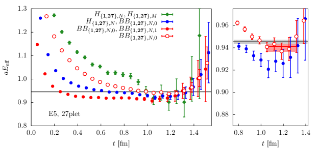
Figure 4: Ground-state effective energy for the singlet (top) and 27-plet (bottom) on ensemble E5 for which SU(3) symmetry is broken. The assignment of a particular multiplet to the energy levels was done on the basis of the dominant overlaps with the interpolating operator. The explanation of symbols is similar to that of Figure 3.

The breaking of SU(3) symmetry induces mixing among the relevant multiplets (singlet, octet and 27-plet), which makes their identification a more involved task. The appropriate strategy is to construct correlator matrices from operators projected onto all relevant flavor multiplets. We recall that the octet can only be represented in terms of two-baryon operators, which, however, cannot be placed at the source when using point-to-all propagators. Therefore, the current analysis is focused only on the singlet and 27-plet states. This deficiency will be rectified by the calculation of hermitian correlator matrices using distillation, described in the next subsection.

In the presence of mixing among different SU(3) multiplets, we have constructed $4\times 4$ correlator matrices from the same combinations of operator types as in the SU(3)-symmetric case, while including both projections onto the singlet and 27-plet.

The matrix correlator and its diagonalization provides us with important information for the interpretation of our results. First, the amount of SU(3) breaking is small, as evidenced by the fact that the geometric mean of the flavor off-diagonal correlators is less than 0.5% of that of the corresponding flavor-diagonal ones. Second, the diagonalization provides clear evidence for the existence of two different low-lying states, although it is not possible to resolve their energy difference with the current statistics. Furthermore, states corresponding to different flavor multiplets can be identified with the help of the eigenvectors computed via the diagonalization procedure. We find that the eigenvectors corresponding to the two low-lying states are dominated by operators in a single multiplet. In this way we can unambiguously assign the energy levels to a particular flavor multiplet.

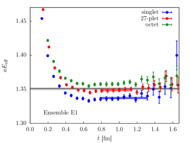
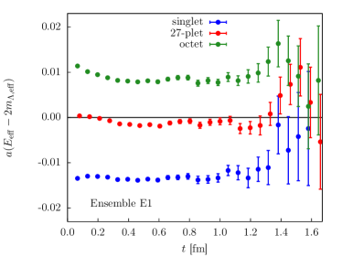
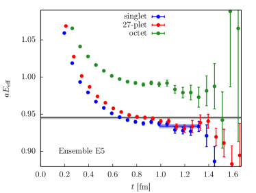
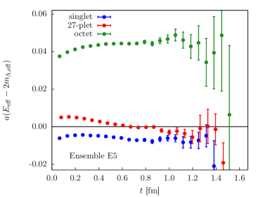
Figure 5: Top: Effective energies for different multiplets for the SU(3)-symmetric case (ensemble E1). The right panel shows the effective energy difference relative to the $\Lambda\Lambda$ threshold. Bottom: energy levels and relative difference for the SU(3)-broken case (ensemble E5). As in Figure 4, the assignment of flavor multiplets to the energy levels was done by means of the dominant overlaps with the interpolating operator. All results have been obtained using distillation. Colored bands indicate the fitted values across the relevant time interval.

Results for the effective energies for the SU(3) singlet and 27-plet are shown in the top and bottom panels of Figure 4, respectively. Data points shown in a given color correspond to a particular choice of sink operators, as indicated in the legend. For both the singlet and the 27-plet, results are similar to what was found for ensemble E1. Effective energies from diagonalizing $4\times 4$ correlator matrices that include two-baryon operators at the sink (filled red and blue circles) dip below the $\Lambda\Lambda$ threshold before $t=0.5$ fm; however, they are in disagreement with each other for $t\lesssim 1.0$ fm. Statistically, the most precise signal is obtained by considering a $2\times 2$ correlator matrix, composed of “narrow” smeared hexaquark interpolating operators for the singlet and 27-plet at the source and a corresponding set of two-baryon operators with both momenta set to zero at the sink. The corresponding effective energy is represented by the open red circles in Figure 4. After fitting the effective energy to a constant in the interval $t=1.0-1.3$ fm we obtain the estimates represented by the red bands in the right panels. We find that the fitted ground-state energies of the singlet and 27-plet are of the order of one standard deviation below the $\Lambda\Lambda$ threshold (see Tables A – A). Note that this analysis is in slight tension with the effective energy from a $4\times 4$ correlator matrix with only two-baryon operators at the sink (filled red circles), meaning that the uncertainty may be somewhat underestimated.

As discussed in Section II.3 we have computed correlation matrices in frames with total momentum $\mathchoice{\mbox{\boldmath$\displaystyle P$}}{\mbox{\boldmath$\textstyle P$}}{\mbox{\boldmath$\scriptstyle P$}}{\mbox{\boldmath$\scriptscriptstyle P$}}=2\pi\mathchoice{\mbox{\boldmath$\displaystyle D$}}{\mbox{\boldmath$\textstyle D$}}{\mbox{\boldmath$\scriptstyle D$}}{\mbox{\boldmath$\scriptscriptstyle D$}}/L$ with $\mathchoice{\mbox{\boldmath$\displaystyle D$}}{\mbox{\boldmath$\textstyle D$}}{\mbox{\boldmath$\scriptstyle D$}}{\mbox{\boldmath$\scriptscriptstyle D$}}^{2}=0,1,2,3$. Estimates for the corresponding ground-state energies are listed in Tables A – A. The combined results in all frames have been used to obtain information on the scattering phase shifts and binding energies in infinite volume. A detailed discussion is deferred to Section IV.

III.2 Dibaryon analysis with distillation

The distillation technique enables the use of two-baryon operators at both the source and the sink. This results in a hermitian correlator matrix and allows us to properly account for the mixing between the singlet, octet and 27-plet states under SU(3) breaking. Within this setup we do not use hexaquark operators. For our initial study, we have computed correlation functions on ensembles E1 and E5 in the rest frame only, which allows for a direct comparison with results from the previous subsection.

As described in Section II.2, we start from the two-baryon interpolating operators of Eqs. (9)–(11), projected on $\mathchoice{\mbox{\boldmath$\displaystyle p$}}{\mbox{\boldmath$\textstyle p$}}{\mbox{\boldmath$\scriptstyle p$}}{\mbox{\boldmath$\scriptscriptstyle p$}}_{1}=\mathchoice{\mbox{\boldmath$\displaystyle p$}}{\mbox{\boldmath$\textstyle p$}}{\mbox{\boldmath$\scriptstyle p$}}{\mbox{\boldmath$\scriptscriptstyle p$}}_{2}=0$. Using the transformation of Appendix B in Ref. Inoue:2010hs we then perform the rotation to the singlet, octet and 27-plet, which yields the operators $BB_{\mathbf{1},L,0}$, $BB_{\mathbf{8},L,0}$ and $BB_{\mathbf{27},L,0}$, respectively. In each channel we compute the corresponding correlation functions and determine the effective energies. Results for the effective energy on E1 are shown in the top left panel of Figure 5. In all three channels, the effective energy approaches a plateau monotonically from above and do not show any of the irregularities observed in the non-hermitian setup based on point-to-all propagators. The top right panel of Figure 5 shows the effective energy difference $E_{\text{eff}}-2m_{\Lambda,\text{eff}}$.

The plot demonstrates that the statistical precision in each of the three individual ($1\times 1$) correlators is sufficient to separate the energy levels corresponding to the singlet, 27-plet and octet channels (in ascending order). The fact that the effective energy differences are nearly constant over time indicates that excited-state contributions in the dibaryon correlation functions are very similar to those in the single $\Lambda$ correlator. Still, it is important to determine the energy difference in the regime where the individual correlators have reached their respective asymptotic behavior. In the singlet channel (color-coded in blue), the effective energy in the plateau region lies significantly below the non-interacting $\Lambda\Lambda$ threshold. The energy level of the 27-plet is closer to the threshold, while the octet state lies significantly above.

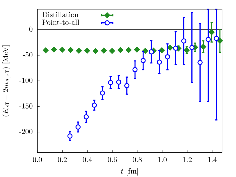
Figure 6: Comparison of the effective energy difference between the singlet ground state and two non-interacting $\Lambda$s, computed with point-to-all propagators and distillation, respectively, for ensemble E1. Open blue circles derive from the same non-hermitian $2\times 2$ correlator matrix that was used to determine the ground state energy in the singlet channel, represented by the blue points in the top panel of Figure 3.

The results on E5 are shown in the lower half of Figure 5, with color coding identical to that of ensemble E1. Due to the breaking of SU(3) symmetry, the different multiplets cannot be treated independently anymore and it is here that the inclusion of the octet operator at the source and sink allows for a consistent treatment of the relevant flavor multiplets. In order to take account of the mixing of different multiplets, we compute a $3\times 3$ correlator matrix using the operators $BB_{\mathbf{1},L,0}$, $BB_{\mathbf{8},L,0}$ and $BB_{\mathbf{27},L,0}$, which is then subjected to the diagonalization procedure. The resulting energy levels are identified with a particular multiplet according to the overlaps with the interpolating operator. The effective energy of the singlet (blue circles) is below the $\Lambda\Lambda$ threshold and, in contrast to the case of point-to-all propagators, can be clearly distinguished from the energy corresponding to two non-interacting $\Lambda$s. The distillation technique allows us to distinguish the singlet and 27-plet as two distinct states with our statistics. The octet, by contrast, lies far above the threshold. For our final estimates of the energies of the different states in the SU(3)-symmetric situation, we have fitted the effective energy to a constant for $t$ starting from 0.8 fm. In the SU(3)-broken situation, the plateau starts later and we have fitted from 1.0 fm.

It is instructive to compare the energy levels computed using point-to-all propagators to the results extracted using the distillation technique. In Figure 6 we show the effective energy gap for the singlet ground state computed on ensemble E1. The plot demonstrates the dramatic improvement in the overall precision provided by the distillation technique in conjunction with LapH smearing: The effective energy gap computed using distillation can be clearly distinguished from zero owing to its tiny statistical errors. Furthermore, it exhibits a flat behavior across a wide range of Euclidean times. While the results obtained using point-to-all propagators are consistent with distillation for $t\gtrsim 0.9$ fm, the larger statistical noise makes it more difficult to determine a non-vanishing energy gap. Also, one does not profit from the partial cancellation of statistical noise in the difference $E_{\rm eff}-2m_{\Lambda,{\rm eff}}$ when using point sources compared to using distillation. As with the point-source method, some caution is required due to the small energy gap to the first excited state. If we assume that the states resemble the noninteracting ones, then the two-baryon operator with both baryons at rest will couple strongly to the ground state and poorly to the elastic excited states; this could explain the long plateau in Figure 6. In fact, the length of this plateau is comparable to the inverse energy gap $\Delta^{-1}\approx 1.1$ fm.

We end this section with a discussion of the relative cost of calculations based on point-to-all propagators and distillation. A simple and fairly accurate cost estimate is provided by the number of propagator solves per configuration. For point sources we have to perform

$$N_{\text{pt}}=N_{\text{flav}}\cdot N_{\text{src}}\cdot N_{\text{smear}}\cdot 12$$ (18)

inversions, where $N_{\text{flav}}$ denotes the number of different quark flavors, $N_{\text{src}}$ is the number of sources, and the number of different smearings is given by $N_{\text{smear}}$. For distillation the number of propagator solves is given by

$$N_{\text{dist}}=N_{\text{flav}}\cdot N_{\text{tsrc}}\cdot N_{\text{LapH}}\cdot 4,$$ (19)

where $N_{\text{tsrc}}$ denotes the number of timeslices used to compute timeslice-to-all propagators, and $N_{\text{LapH}}$ is the number of low-lying modes of the spatial Laplacian. Using the information from Table 1 and the fact that we have used $N_{\text{LapH}}=56$ modes, we find $N_{\text{pt}}=3072$ and $N_{\text{dist}}=1792$ for ensemble E1. For E5 the above expressions evaluate to $N_{\text{pt}}=1536$ and $N_{\text{dist}}=1792$. We conclude that the better data quality of the distillation technique is achieved for comparable or even lower cost. For a more precise cost comparison one should also take into account that the cost of contractions in the distillation approach is typically larger. The associated computational overhead may become significant on large volumes. We will present a more thorough discussion of this issue in a future publication.

IV Finite volume analysis

The finite-volume rest frame energy level $E$, when below the two-particle threshold, provides a naïve estimate of the mass of the bound state. However, this can suffer from significant finite-volume effects that are asymptotically only suppressed as $e^{-\kappa L}$, where $\kappa$ is the binding momentum defined via $E=2\sqrt{m_{\Lambda}^{2}-\kappa^{2}}$. In addition, there can be an energy level below threshold without a bound state, in which case it has a power-law dependence on $L$ that depends on the scattering length.

For a more careful study of the presence of a bound state and its mass, we turn to Lüscher’s finite volume quantization condition Luscher:1990ux and its extension to moving frames Rummukainen:1995vs . Below the three-particle threshold, this is a relation between the two-particle scattering amplitude and the finite-volume energy levels. In the case of one pair of identical particles scattering in the $S$ wave, if we ignore the influence of higher partial waves due to the breaking of rotational symmetry, the condition takes the form

$$p\cot\delta(p)=\frac{2}{\sqrt{\pi}L\gamma}Z_{00}^{\mathbf{D}}\left(1,\left(\frac{pL}{2\pi}\right)^{2}\right),$$ (20)

where $p$ is the scattering momentum satisfying $E_{\text{cm}}\equiv\sqrt{E^{2}-\mathchoice{\mbox{\boldmath$\displaystyle P$}}{\mbox{\boldmath$\textstyle P$}}{\mbox{\boldmath$\scriptstyle P$}}{\mbox{\boldmath$\scriptscriptstyle P$}}^{2}}=2\sqrt{m_{\Lambda}^{2}+p^{2}}$, $\delta(p)$ is the scattering phase shift, $\gamma=E/E_{\text{cm}}$ is the moving-frame boost factor, and $Z_{00}^{\mathbf{D}}$ is a generalized zeta function defined in Ref. Rummukainen:1995vs . Our numerical implementation of the zeta function is based on Ref. Gockeler:2012yj .

As recently reviewed in Ref. Iritani:2017rlk , a bound state, corresponding to a pole in the scattering amplitude on the real $p^{2}$ axis below zero, is determined by the condition $p\cot\delta(p)=-\sqrt{-p^{2}}$. That reference also provides a check that can be applied to lattice data: at the pole, the slope of $p\cot\delta(p)$ (versus $p^{2}$) must be smaller than that of $-\sqrt{-p^{2}}$.

For small $p^{2}$, the phase shift can be described by the effective range expansion. We use the first two terms,

$$p\cot\delta(p)=-\frac{1}{a_{0}}+\frac{r_{0}}{2}p^{2},$$ (21)

where $a_{0}$ is the scattering length and $r_{0}$ is the effective range. Fitting this to lattice data is not a simple linear fit, since $p\cot\delta(p)$ and $p^{2}$ are not independent variables, being related by the quantization condition. We choose to fit to the squared scattering momentum $p^{2}$ determined from each lattice energy, in a manner similar to what was done for fitting to the lattice energies in Ref. Erben:2017hvr . Fitting to the momentum rather than energy benefits from cancellations of statistical uncertainties that are correlated between $E$ and $m_{\Lambda}$. Given a set of fit parameters $(a_{0},r_{0})$, in each frame the fit momentum is determined by finding the solution to the quantization condition that is nearest to the corresponding momentum determined from the lattice calculation, i.e. by numerically solving

$$\frac{2}{\sqrt{\pi}L\gamma}Z_{00}^{\mathbf{D}}\left(1,\left(\frac{pL}{2\pi}\right)^{2}\right)=-\frac{1}{a_{0}}+\frac{r_{0}}{2}p^{2}.$$ (22)

We only consider the ensembles with SU(3) symmetry, since otherwise this is a much more complicated coupled-channel ($\Lambda\Lambda$, $N\Xi$, and $\Sigma\Sigma$) system.

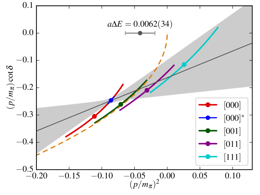
Figure 7: SU(3) singlet scattering phase shift on ensemble E1. The legend indicates the moving frame $\mathchoice{\mbox{\boldmath$\displaystyle D$}}{\mbox{\boldmath$\textstyle D$}}{\mbox{\boldmath$\scriptstyle D$}}{\mbox{\boldmath$\scriptscriptstyle D$}}=\tfrac{L}{2\pi}\mathchoice{\mbox{\boldmath$\displaystyle P$}}{\mbox{\boldmath$\textstyle P$}}{\mbox{\boldmath$\scriptstyle P$}}{\mbox{\boldmath$\scriptscriptstyle P$}}$; the data point labeled $[000]^{*}$ was obtained using distillation and the others were obtained using point-source data. The grey line and its error band indicate the effective-range-expansion fit, and the orange dashed curve corresponds to $p\cot\delta=-\sqrt{-p^{2}}$. The horizontal error bar shows the intersection between the grey line and the orange dashed curve, which is translated to a binding energy in the label above it.

We are only able to obtain a reliable fit in the flavor singlet sector on ensemble E1, where the precise energy level in the rest frame from the distillation method provides a stronger constraint than the other data. This is shown in Figure 7; we find the scattering length to be 1.3(5) fm and the effective range 0.4(3) fm. There is a clear intersection with the bound-state curve, which has a slope with the correct behavior, indicating the presence of a bound $H$ dibaryon. This intersection yields a binding energy of $\Delta E=19(10)$ MeV, somewhat smaller in magnitude than the naïve value obtained from the rest-frame energy difference $2m_{\Lambda}-E$.

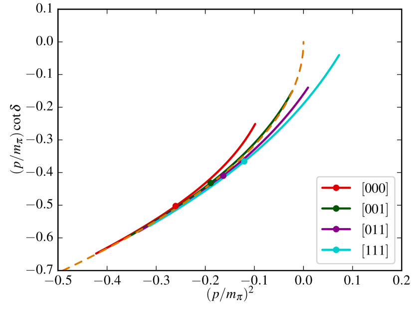
Figure 8: SU(3) singlet scattering phase shift on ensemble A1. The legend indicates the moving frame $\mathchoice{\mbox{\boldmath$\displaystyle D$}}{\mbox{\boldmath$\textstyle D$}}{\mbox{\boldmath$\scriptstyle D$}}{\mbox{\boldmath$\scriptscriptstyle D$}}=\tfrac{L}{2\pi}\mathchoice{\mbox{\boldmath$\displaystyle P$}}{\mbox{\boldmath$\textstyle P$}}{\mbox{\boldmath$\scriptstyle P$}}{\mbox{\boldmath$\scriptscriptstyle P$}}$ and the orange dashed curve corresponds to $p\cot\delta=-\sqrt{-p^{2}}$.

For the ensembles A1 and N1, we are unable to obtain reliable fits. However, in the flavor singlet sector, the data in the rest frame and in the higher moving frames sit on opposite sides of the bound-state curve, which indicates that there will be an intersection between it and the phase shift; see Figure 8. For the frame $\mathchoice{\mbox{\boldmath$\displaystyle D$}}{\mbox{\boldmath$\textstyle D$}}{\mbox{\boldmath$\scriptstyle D$}}{\mbox{\boldmath$\scriptscriptstyle D$}}^{2}=1$, the point — together with its error along the quantization curve — is almost on top of the bound-state curve, and therefore we make a conservative estimate of the binding energy. To this end we consider the interval defined by the maximum and minimum values of $E_{\text{cm}}$ deduced from the frames with $\mathchoice{\mbox{\boldmath$\displaystyle D$}}{\mbox{\boldmath$\textstyle D$}}{\mbox{\boldmath$\scriptstyle D$}}{\mbox{\boldmath$\scriptscriptstyle D$}}^{2}=0,1$. The midpoint of this interval is identified with the central value of the binding energy, while the $1\sigma$ error is defined as the difference with the upper and lower bounds. For N1, we get $a\Delta E=0.016(13)$, or 65(53) MeV. For A1, we get $a\Delta E=0.028(25)$, or 73(66) MeV.

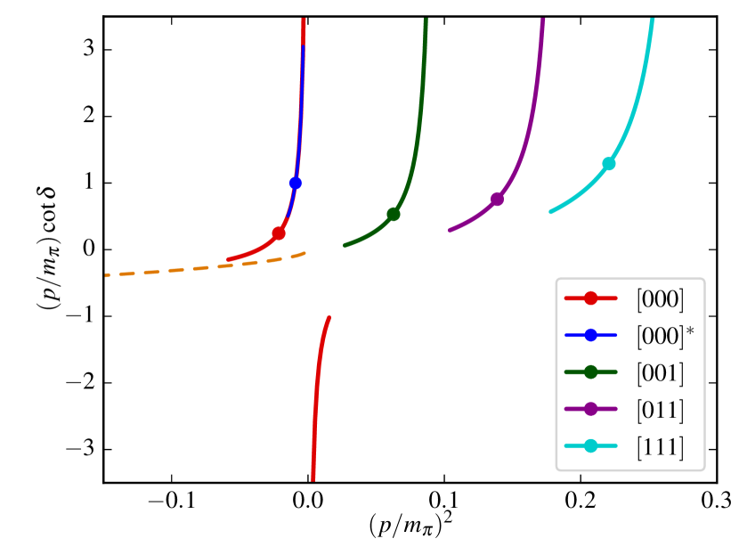
Figure 9: SU(3) 27-plet scattering phase shift on ensemble E1. The legend indicates the moving frame $\mathchoice{\mbox{\boldmath$\displaystyle D$}}{\mbox{\boldmath$\textstyle D$}}{\mbox{\boldmath$\scriptstyle D$}}{\mbox{\boldmath$\scriptscriptstyle D$}}=\tfrac{L}{2\pi}\mathchoice{\mbox{\boldmath$\displaystyle P$}}{\mbox{\boldmath$\textstyle P$}}{\mbox{\boldmath$\scriptstyle P$}}{\mbox{\boldmath$\scriptscriptstyle P$}}$; the data point labeled $[000]^{*}$ was obtained using distillation and the others were obtained using point-source data. The orange dashed curve corresponds to $p\cot\delta=-\sqrt{-p^{2}}$.

In the 27-plet sector, our data are generally not precise enough to distinguish the energy levels from the noninteracting ones; this means that the phase shift is consistent with zero. On E1, where distillation provides a relatively precise value, the rest-frame energy is slightly below threshold. Using the quantization condition, we find that just below threshold, $p\cot\delta$ is probably positive; see Figure 9. This means that a bound state (which would be a dineutron) is unlikely, however an intersection with $p\cot\delta=+\sqrt{-p^{2}}$, which corresponds to a virtual bound state (i.e., a pole on the unphysical sheet), is possible. If we neglect the dependence on $p^{2}$, the distillation energy level implies a scattering length $a_{0}=-0.2_{-0.2}^{+0.1}$ fm. However, note that the quantization condition is very nonlinear and at 3$\sigma$ the statistical uncertainty on $a_{0}$ becomes as large as ${}^{+0.3}_{-1.2}$, assuming a symmetric Gaussian uncertainty on the $p^{2}$ determined from the energy level.

V Discussion and Conclusion

We have presented a detailed study of the spectrum of the $H$ dibaryon in the SU(3) flavor-symmetric and broken cases, using lattice QCD simulations with dynamical up and down quarks and a quenched strange quark. We have analyzed the efficiency of different interpolating operators in the determination of hadronic finite volume energy eigenvalues via variational analysis.

Our findings indicate that point-like hexaquark operators provide a poor overlap onto the SU(3) singlet ground state. This becomes evident through the slow convergence to the ground state plateau seen in the time dependence of the lowest energy eigenvalue. The inclusion of bilocal two-baryon operators at the sink improves the overlap considerably, as indicated by an earlier onset of the plateau and a stronger statistical signal. However, in a setup based on point-to-all propagators, the improvement comes at the expense of having to deal with non-hermitian correlator matrices. As a consequence, effective energies determined from the eigenvalues are not guaranteed to approach their asymptotic behavior from above. In this way an additional systematic is introduced, as the onset of the plateau is obscured or can be misidentified.

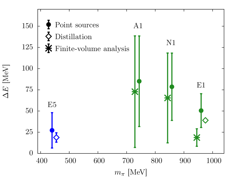
Figure 10: Summary of our results for the binding energy of the $H$ dibaryon. Green and blue colors refer to the SU(3)-symmetric and broken cases, respectively. Full circles and open diamonds represent results obtained in the rest frame using point sources and distillation, respectively. Crosses denote estimates for the binding energy extracted from the finite-volume analysis of results in different frames as described in Section IV.

A fully hermitian setup with bilocal two-baryon operators at both the source and sink can be realized with the help of the distillation technique which allows for the calculation of timeslice-to-all propagators. In our study of the SU(3) symmetric and broken cases we have been able to determine the energy levels reliably and with good statistical precision for the flavor singlet, 27-plet and octet.

In particular, we could identify a clear gap between the ground-state singlet energy level and the $2m_{\Lambda}$ threshold, which suggests that there is a bound $H$ dibaryon. The energy difference provides a naïve estimate of the binding energy, ${\Delta}E\equiv 2m_{\Lambda}-E$. For ensembles E1 and E5, which realize the SU(3) symmetric and broken situations respectively, the estimates are

E1: $$\Delta E=39.0\pm 2.2\,\text{MeV},\quad m_{\pi}=960\,\text{MeV},$$ (23)

E5: $$\Delta E=18.8\pm 5.5\,\text{MeV},\quad m_{\pi}=440\,\text{MeV}.$$ (24)

However, recalling that finite-volume effects are asymptotically suppressed as $e^{-{\kappa}L}$, where $\kappa$ is the binding momentum, the naïve estimates of the binding energy in Eqs. (23) and (24) may not be very reliable, given that ${\kappa}L$ evaluates to 2.99(8) for E1 and 1.74(25) for E5.

In addition, we have applied Lüscher’s finite-volume quantization condition to determine the scattering phase shift, which we use to obtain a more reliable estimate of the binding energy. Including data from the rest frame as well as several moving frames in the finite-volume analysis of the singlet case results in a shallower binding energy compared to the naïve estimate:

$$\text{E1:}\quad\Delta E=19\pm 10\,\text{MeV},\quad m_{\pi}=960\,\text{MeV}.$$ (25)

Repeating the analysis for the SU(3) 27-plet is made more difficult through the relative closeness of the energy levels to the non-interacting levels, and the same is true in the case of broken SU(3)-flavor symmetry. We expect the situation to improve in our ongoing work, since we will obtain more precise results by also using distillation in the moving frames.

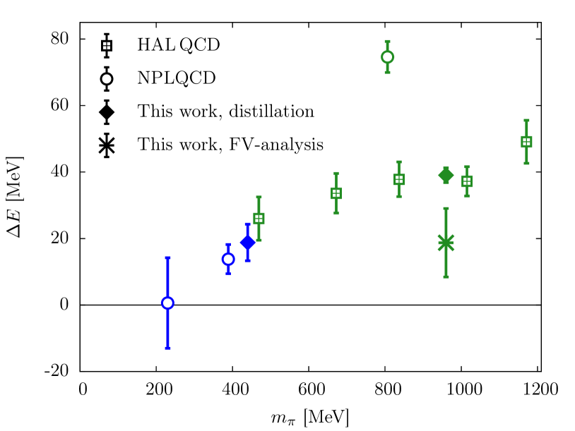
Figure 11: Comparison of our results in Eqs. (23)–(25) to the estimates quoted by NPLQCD Beane:2010hg ; Beane:2011zpa ; Beane:2012vq and HAL QCD Inoue:2010es ; Inoue:2011ai . Green and blue symbols refer to the SU(3)-symmetric and broken cases, respectively. The data point marked by a star denotes the result in infinite volume.

In Figure 10 we show a compilation of our results for the binding energy on all our ensembles, plotted against the pion mass. The comparison with the estimates of the NPLQCD Beane:2010hg ; Beane:2011zpa ; Beane:2012vq and HAL QCD Inoue:2010es ; Inoue:2011ai collaborations is made in Figure 11. In the SU(3)-symmetric case we find that our estimate is considerably smaller than the result quoted by NPLQCD at a similar value of the pion mass Beane:2010hg . Potentially, uncontrolled systematics such as the incorrect identification of the plateau, quenching of the strange quark or finite-volume effects could be the source of this discrepancy. We will address these issues in a future publication based on ensembles with $N_{\text{f}}=2+1$ flavors of dynamical quarks.

Our findings suggest that the combination of distillation and Lüscher’s finite-volume formalism will allow for a considerably improved calculation of the binding energy. Thus, there are good prospects for a reliable determination of this quantity at the physical point.

Appendix A Fit results

In Tables A and 3 we provide our mass estimates for single baryons in the SU(3)-symmetric and broken cases, respectively. Dibaryon energy levels, as determined from fits to the effective energy, are listed in Tables A and A. The corresponding energy difference with the $\Lambda\Lambda$ threshold is shown in Tables A and A.

Table 2: Mass estimates of the $\Lambda$ hyperon (in lattice units) in the SU(3)-symmetric case. The rightmost column shows the fit range. Ensembles marked by an asterisk represent results determined distillation and LapH smearing.

Ensemble	$am_{\Lambda}$	Fit range
$\text{A1}$	0.6560(23)	[16,25]
$\text{E1}$	0.6763(09)	[15,20]
$\text{E1}^{*}$	0.6751(09)	[12,20]
$\text{N1}$	0.4538(20)	[25,38]

The fitted mass estimates for the octet baryons, obtained using either point sources or distillation, differ at the level of about two standard deviations (see Table 3). As can be inferred easily from Fig. 12, the effective masses obtained using either type of source agree within errors, and hence the differences observed among the estimates in Table 3 are commensurate with statistical fluctuations.

Table 3: Mass estimates of octet baryons on ensemble E5, which corresponds to the SU(3)-broken situation. We list the results obtained using point sources and distillation, the latter being indicated by an asterisk. The estimates are in lattice units along with the relevant fit ranges.

	E5	Fit range	E5∗	Fit range
$am_{N}$	0.4330(11)	[15,25]	0.4302(15)	[15,21]
$am_{\Lambda}$	0.4727(07)	[15,25]	0.4701(10)	[15,21]
$am_{\Sigma}$	0.4893(08)	[15,25]	0.4870(11)	[15,21]
$am_{\Xi}$	0.5201(05)	[15,25]	0.5181(07)	[15,21]

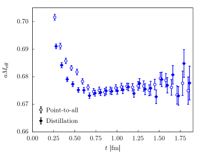
Figure 12: Left: Effective masses for the $\Lambda$ hyperon in the SU(3)-symmetric case (ensemble E1). Right: effective masses for octet baryons, i.e. the nucleon, $\Lambda$, $\Sigma$ and $\Xi$ in the SU(3)-broken case (ensemble E5). Diamonds and open circles denote results obtained using distillation and point sources, respectively. For the latter, the narrow smearing width was used (see Section II.2).

Table 4: Fitted energies of the ground state for the singlet. Results determined using distillation are listed in rows labeled E$1^{*}$ and E$5^{*}$.

Ensemble	$\mathchoice{\mbox{\boldmath$\displaystyle D$}}{\mbox{\boldmath$\textstyle D$}}{\mbox{\boldmath$\scriptstyle D$}}{\mbox{\boldmath$\scriptscriptstyle D$}}^{2}=0$		$\mathchoice{\mbox{\boldmath$\displaystyle D$}}{\mbox{\boldmath$\textstyle D$}}{\mbox{\boldmath$\scriptstyle D$}}{\mbox{\boldmath$\scriptscriptstyle D$}}^{2}=1$		$\mathchoice{\mbox{\boldmath$\displaystyle D$}}{\mbox{\boldmath$\textstyle D$}}{\mbox{\boldmath$\scriptstyle D$}}{\mbox{\boldmath$\scriptscriptstyle D$}}^{2}=2$		$\mathchoice{\mbox{\boldmath$\displaystyle D$}}{\mbox{\boldmath$\textstyle D$}}{\mbox{\boldmath$\scriptstyle D$}}{\mbox{\boldmath$\scriptscriptstyle D$}}^{2}=3$
	$aE_{\text{singlet}}$	Fit range	$aE_{\text{singlet}}$	Fit range	$aE_{\text{singlet}}$	Fit range	$aE_{\text{singlet}}$	Fit range
$\text{E1}$	$1.3358(66)$	[14,21]	$1.3562(58)$	[13,19]	$1.3763(60)$	[12,19]	$1.3985(74)$	[12,19]
$\text{E1}^{*}$	$1.3371(18)$	[12,20]	-	-	-	-	-	-
$\text{A1}$	$1.279(20)$	[11,16]	$1.303(20)$	[11,17]	$1.321(21)$	[11,15]	$1.341(23)$	[11,15]
$\text{N1}$	$0.888(10)$	[20,27]	$0.904(11)$	[20,27]	$0.9170(77)$	[18,23]	$0.9341(53)$	[16,21]
$\text{E5}$	$0.9363(70)$	[15,19]	$0.9659(68)$	[15,19]	$0.974(16)$	[17,20]	$0.985(20)$	[17,21]
$\text{E5}^{*}$	$0.9340(26)$	[15,20]	-	-	-	-	-	-

Table 5: Ground-state energy differences $a(2m_{\Lambda}-E_{\text{cm}})$ for the singlet. Results determined using distillation are listed in rows labeled E$1^{*}$ and E$5^{*}$. The rightmost column contains the results for the binding energy determined via Lüscher’s finite-volume formalism.

Ensemble	$\mathchoice{\mbox{\boldmath$\displaystyle D$}}{\mbox{\boldmath$\textstyle D$}}{\mbox{\boldmath$\scriptstyle D$}}{\mbox{\boldmath$\scriptscriptstyle D$}}^{2}=0$	$\mathchoice{\mbox{\boldmath$\displaystyle D$}}{\mbox{\boldmath$\textstyle D$}}{\mbox{\boldmath$\scriptstyle D$}}{\mbox{\boldmath$\scriptscriptstyle D$}}^{2}=1$	$\mathchoice{\mbox{\boldmath$\displaystyle D$}}{\mbox{\boldmath$\textstyle D$}}{\mbox{\boldmath$\scriptstyle D$}}{\mbox{\boldmath$\scriptscriptstyle D$}}^{2}=2$	$\mathchoice{\mbox{\boldmath$\displaystyle D$}}{\mbox{\boldmath$\textstyle D$}}{\mbox{\boldmath$\scriptstyle D$}}{\mbox{\boldmath$\scriptscriptstyle D$}}^{2}=3$	FV analysis
$\text{E1}$	$0.0168(66)$	$0.0107(60)$	$0.0047(62)$	$-0.0039(77)$	0.0062(34)
$\text{E1}^{*}$	$0.0130(7)$	-	-	-
$\text{A1}$	$0.033(20)$	$0.024(21)$	$0.020(22)$	$0.015(24)$	0.028(25)0
$\text{N1}$	$0.019(10)$	$0.014(11)$	$0.009(7)$	$0.001(5)$	0.016(13)0
$\text{E5}$	$0.0091(69)$	$-0.0004(68)$	$0.0118(164)$	$0.0214(214)$	-
$\text{E5}^{*}$	$0.0063(18)$	-	-	-

Table 6: Fitted energies of the ground state for the 27-plet. Results determined using distillation are listed in the row labeled E$1^{*}$.

Ensemble	$\mathchoice{\mbox{\boldmath$\displaystyle D$}}{\mbox{\boldmath$\textstyle D$}}{\mbox{\boldmath$\scriptstyle D$}}{\mbox{\boldmath$\scriptscriptstyle D$}}^{2}=0$		$\mathchoice{\mbox{\boldmath$\displaystyle D$}}{\mbox{\boldmath$\textstyle D$}}{\mbox{\boldmath$\scriptstyle D$}}{\mbox{\boldmath$\scriptscriptstyle D$}}^{2}=1$		$\mathchoice{\mbox{\boldmath$\displaystyle D$}}{\mbox{\boldmath$\textstyle D$}}{\mbox{\boldmath$\scriptstyle D$}}{\mbox{\boldmath$\scriptscriptstyle D$}}^{2}=2$		$\mathchoice{\mbox{\boldmath$\displaystyle D$}}{\mbox{\boldmath$\textstyle D$}}{\mbox{\boldmath$\scriptstyle D$}}{\mbox{\boldmath$\scriptscriptstyle D$}}^{2}=3$
	$aE_{\text{27-plet}}$	Fit range	$aE_{\text{27-plet}}$	Fit range	$aE_{\text{27-plet}}$	Fit range	$aE_{\text{27-plet}}$	Fit range
$\text{E1}$	$1.3494(58)$	[14,20]	$1.3761(54)$	[13,19]	$1.4011(51)$	[12,19]	$1.4265(61)$	[12,16]
$\text{E1}^{*}$	$1.3488(19)$	[12,17]	-	-	-	-	-	-
$\text{A1}$	$1.318(11)$	[12,18]	$1.346(12)$	[12,18]	$1.367(12)$	[10,16]	$1.394(15)$	[10,16]
$\text{N1}$	$0.9058(68)$	[21,29]	$0.9205(83)$	[22,29]	$0.9366(93)$	[22,28]	$0.953(11)$	[22,29]
$\text{E5}$	$0.9412(48)$	[16,20]	$0.9843(48)$	[16,20]	$1.0299(66)$	[16,20]	$1.0789(94)$	[16,20]
$\text{E5}^{*}$	$0.9380(25)$	[15,20]	-	-	-	-	-	-

Table 7: Ground-state energy differences $a(2m_{\Lambda}-E_{\text{cm}})$ for the 27-plet. Results determined using distillation are listed in the row labeled E$1^{*}$.

Ensemble	$\mathchoice{\mbox{\boldmath$\displaystyle D$}}{\mbox{\boldmath$\textstyle D$}}{\mbox{\boldmath$\scriptstyle D$}}{\mbox{\boldmath$\scriptscriptstyle D$}}^{2}=0$	$\mathchoice{\mbox{\boldmath$\displaystyle D$}}{\mbox{\boldmath$\textstyle D$}}{\mbox{\boldmath$\scriptstyle D$}}{\mbox{\boldmath$\scriptscriptstyle D$}}^{2}=1$	$\mathchoice{\mbox{\boldmath$\displaystyle D$}}{\mbox{\boldmath$\textstyle D$}}{\mbox{\boldmath$\scriptstyle D$}}{\mbox{\boldmath$\scriptscriptstyle D$}}^{2}=2$	$\mathchoice{\mbox{\boldmath$\displaystyle D$}}{\mbox{\boldmath$\textstyle D$}}{\mbox{\boldmath$\scriptstyle D$}}{\mbox{\boldmath$\scriptscriptstyle D$}}^{2}=3$
$\text{E1}$	$0.0032(56)$	$-0.0094(53)$	$-0.0207(51)$	$-0.0328(63)$
$\text{E1}^{*}$	$0.0014(8)$	-	-	-
$\text{A1}$	$-0.006(11)$	$-0.019(12)$	$-0.027(13)$	$-0.040(16)$
$\text{N1}$	$0.002(6)$	$-0.004(7)$	$-0.011(9)$	$-0.018(10)$
$\text{E5}$	$0.0042(46)$	$-0.0191(47)$	$-0.0464(67)$	$-0.0785(98)$
$\text{E5}^{*}$	$0.0023(17)$	-	-	-

References

- (1) R. F. Lebed, R. E. Mitchell, and E. S. Swanson, “Heavy-Quark QCD Exotica,” Prog. Part. Nucl. Phys. 93 (2017) 143–194, arXiv:1610.04528 [hep-ph].
- (2) LHCb Collaboration, R. Aaij et al., “Observation of Resonances Consistent with Pentaquark States in Decays,” Phys. Rev. Lett. 115 (2015) 072001, arXiv:1507.03414 [hep-ex].
- (3) R. L. Jaffe, “Perhaps a stable dihyperon,” Phys. Rev. Lett. 38 (1977) 195–198. [Erratum: Phys. Rev. Lett. 38, 617 (1977)].
- (4) H. Takahashi et al., “Observation of a double hypernucleus,” Phys. Rev. Lett. 87 (2001) 212502.
- (5) KEK-E176, E373, and J-PARC-E07 Collaboration, K. Nakazawa, “Double- hypernuclei via the hyperon capture at rest reaction in a hybrid emulsion,” Nucl. Phys. A 835 (2010) 207–214.
- (6) Belle Collaboration, B. H. Kim et al., “Search for an -dibaryon with mass near in and decays,” Phys. Rev. Lett. 110 (2013) 222002, arXiv:1302.4028 [hep-ex].
- (7) P. B. Mackenzie and H. B. Thacker, “Evidence against a stable dibaryon from lattice QCD,” Phys. Rev. Lett. 55 (1985) 2539.
- (8) Y. Iwasaki, T. Yoshie, and Y. Tsuboi, “The dibaryon in lattice QCD,” Phys. Rev. Lett. 60 (1988) 1371–1374.
- (9) Z.-H. Luo, M. Loan, and X.-Q. Luo, “H-dibaryon from lattice QCD with improved anisotropic actions,” Mod. Phys. Lett. A22 (2007) 591–597, arXiv:0803.3171 [hep-lat].
- (10) Z.-H. Luo, M. Loan, and Y. Liu, “Search for the dibaryon on the lattice,” Phys. Rev. D 84 (2011) 034502, arXiv:1106.1945 [hep-lat].
- (11) A. Pochinsky, J. W. Negele, and B. Scarlet, “Lattice study of the dibaryon,” Nucl. Phys. Proc. Suppl. 73 (1999) 255–257, arXiv:hep-lat/9809077 [hep-lat].
- (12) I. Wetzorke, F. Karsch, and E. Laermann, “Further evidence for an unstable H dibaryon?,” Nucl. Phys. Proc. Suppl. 83 (2000) 218–220, arXiv:hep-lat/9909037 [hep-lat].
- (13) I. Wetzorke and F. Karsch, “The H dibaryon on the lattice,” Nucl. Phys. Proc. Suppl. 119 (2003) 278–280, arXiv:hep-lat/0208029 [hep-lat].
- (14) S. R. Beane et al., “Present constraints on the H-dibaryon at the physical point from lattice QCD,” Mod. Phys. Lett. A 26 (2011) 2587–2595, arXiv:1103.2821 [hep-lat].
- (15) A. Francis, C. Miao, T. D. Rae, and H. Wittig, “Two-baryon correlation functions in 2-flavour QCD,” PoS LATTICE2013 (2014) 440, arXiv:1311.3933 [hep-lat].
- (16) J. Green, A. Francis, P. Junnarkar, C. Miao, T. Rae, and H. Wittig, “Search for a bound H-dibaryon using local six-quark interpolating operators,” PoS LATTICE2014 (2014) 107, arXiv:1411.1643 [hep-lat].
- (17) P. Junnarkar, A. Francis, J. Green, C. Miao, T. Rae, and H. Wittig, “Search for the H-dibaryon in two flavor lattice QCD,” PoS CD15 (2015) 079, arXiv:1511.01849 [hep-lat]. [PoS LATTICE2015, 082 (2016)].
- (18) NPLQCD Collaboration, S. R. Beane et al., “Evidence for a bound dibaryon from lattice QCD,” Phys. Rev. Lett. 106 (2011) 162001, arXiv:1012.3812 [hep-lat].
- (19) NPLQCD Collaboration, S. R. Beane, E. Chang, W. Detmold, H. W. Lin, T. C. Luu, K. Orginos, A. Parreño, M. J. Savage, A. Torok, and A. Walker-Loud, “The deuteron and exotic two-body bound states from lattice QCD,” Phys. Rev. D 85 (2012) 054511, arXiv:1109.2889 [hep-lat].
- (20) NPLQCD Collaboration, S. R. Beane, E. Chang, S. D. Cohen, W. Detmold, H. W. Lin, T. C. Luu, K. Orginos, A. Parreño, M. J. Savage, and A. Walker-Loud, “Light nuclei and hypernuclei from quantum chromodynamics in the limit of SU(3) flavor symmetry,” Phys. Rev. D 87 (2013) 034506, arXiv:1206.5219 [hep-lat].
- (21) HAL QCD Collaboration, T. Inoue, N. Ishii, S. Aoki, T. Doi, T. Hatsuda, Y. Ikeda, K. Murano, H. Nemura, and K. Sasaki, “Baryon-baryon interactions in the flavor SU(3) limit from full QCD simulations on the lattice,” Prog. Theor. Phys. 124 (2010) 591–603, arXiv:1007.3559 [hep-lat].
- (22) HAL QCD Collaboration, T. Inoue, N. Ishii, S. Aoki, T. Doi, T. Hatsuda, Y. Ikeda, K. Murano, H. Nemura, and K. Sasaki, “Bound dibaryon in flavor SU(3) limit of lattice QCD,” Phys. Rev. Lett. 106 (2011) 162002, arXiv:1012.5928 [hep-lat].
- (23) HAL QCD Collaboration, T. Inoue, S. Aoki, T. Doi, T. Hatsuda, Y. Ikeda, N. Ishii, K. Murano, H. Nemura, and K. Sasaki, “Two-baryon potentials and -dibaryon from 3-flavor lattice QCD simulations,” Nucl. Phys. A 881 (2012) 28–43, arXiv:1112.5926 [hep-lat].
- (24) K. Sasaki et al., “First results of baryon interactions from lattice QCD with physical masses (3) – Strangeness two-baryon system,” PoS LATTICE2015 (2016) 088.
- (25) K. Sasaki, S. Aoki, T. Doi, S. Gongyo, T. Hatsuda, Y. Ikeda, T. Inoue, T. Iritani, N. Ishii, and T. Miyamoto, “Lattice QCD studies on baryon interactions in the strangeness -2 sector with physical quark masses,” EPJ Web Conf. 175 (2018) 05010.
- (26) J. Haidenbauer and U.-G. Meissner, “To bind or not to bind: The H-dibaryon in light of chiral effective field theory,” Phys. Lett. B706 (2011) 100–105, arXiv:1109.3590 [hep-ph].
- (27) J. Haidenbauer and U. G. Meissner, “Exotic bound states of two baryons in light of chiral effective field theory,” Nucl. Phys. A881 (2012) 44–61, arXiv:1111.4069 [nucl-th].
- (28) C. Michael, “Adjoint Sources in Lattice Gauge Theory,” Nucl. Phys. B259 (1985) 58–76.
- (29) M. Lüscher and U. Wolff, “How to calculate the elastic scattering matrix in two-dimensional quantum field theories by numerical simulation,” Nucl. Phys. B 339 (1990) 222–252.
- (30) B. Blossier, M. Della Morte, G. von Hippel, T. Mendes, and R. Sommer, “On the generalized eigenvalue method for energies and matrix elements in lattice field theory,” JHEP 04 (2009) 094.
- (31) Hadron Spectrum Collaboration, M. Peardon, J. Bulava, J. Foley, C. Morningstar, J. Dudek, R. G. Edwards, B. Joo, H.-W. Lin, D. G. Richards, and K. J. Juge, “A Novel quark-field creation operator construction for hadronic physics in lattice QCD,” Phys. Rev. D 80 (2009) 054506, arXiv:0905.2160 [hep-lat].
- (32) S. Aoki et al., “Review of lattice results concerning low-energy particle physics,” Eur. Phys. J. C77 no. 2, (2017) 112, arXiv:1607.00299 [hep-lat].
- (33) B. Sheikholeslami and R. Wohlert, “Improved Continuum Limit Lattice Action for QCD with Wilson Fermions,” Nucl. Phys. B259 (1985) 572.
- (34) M. Lüscher, “Schwarz-preconditioned HMC algorithm for two-flavour lattice QCD,” Comput. Phys. Commun. 165 (2005) 199–220, arXiv:hep-lat/0409106 [hep-lat].
- (35) M. Lüscher, “Deflation acceleration of lattice QCD simulations,” JHEP 12 (2007) 011, arXiv:0710.5417 [hep-lat].
- (36) M. Marinkovic and S. Schaefer, “Comparison of the mass preconditioned HMC and the DD-HMC algorithm for two-flavour QCD,” PoS LATTICE2010 (2010) 031, arXiv:1011.0911 [hep-lat].
- (37) ALPHA Collaboration, K. Jansen and R. Sommer, “O() improvement of lattice QCD with two flavors of Wilson quarks,” Nucl. Phys. B530 (1998) 185–203, arXiv:hep-lat/9803017 [hep-lat]. [Erratum: Nucl. Phys. B643 (2002) 517].
- (38) P. Fritzsch, F. Knechtli, B. Leder, M. Marinkovic, S. Schaefer, R. Sommer, and F. Virotta, “The strange quark mass and Lambda parameter of two flavor QCD,” Nucl. Phys. B865 (2012) 397–429, arXiv:1205.5380 [hep-lat].
- (39) M. Lüscher and S. Schaefer, “OpenQCD.” http://luscher.web.cern.ch/luscher/openQCD/.
- (40) A. Stathopoulos and J. R. McCombs, “PRIMME: PReconditioned Iterative MultiMethod Eigensolver: Methods and software description,” ACM Transactions on Mathematical Software 37 no. 2, (2010) 21:1–21:30.
- (41) SciDAC, LHPC, UKQCD Collaboration, R. G. Edwards and B. Joó, “The Chroma software system for lattice QCD,” Nucl. Phys. Proc. Suppl. 140 (2005) 832, arXiv:hep-lat/0409003 [hep-lat].
- (42) T. Blum, T. Izubuchi, and E. Shintani, “New class of variance-reduction techniques using lattice symmetries,” Phys. Rev. D 88 (2013) 094503, arXiv:1208.4349 [hep-lat].
- (43) E. Golowich, J. Donoghue, and B. R. Holstein, “Weak Decays of the Dibaryon,” Phys. Rev. D 34 (1986) 3434.
- (44) E. Golowich and T. Sotirelis, “O() mass contributions to the dibaryon in a truncated bag model,” Phys. Rev. D 46 (1992) 354–363.
- (45) R. L. Jaffe, “Exotica,” Phys. Rept. 409 (2005) 1–45, arXiv:hep-ph/0409065 [hep-ph].
- (46) S. Güsken, “A Study of smearing techniques for hadron correlationfunctions,” Nucl. Phys. Proc. Suppl. 17 (1990) 361–364.
- (47) APE Collaboration, M. Albanese et al., “Glueball Masses and String Tension in Lattice QCD,” Phys. Lett. B192 (1987) 163–169.
- (48) C. Morningstar and M. J. Peardon, “Analytic smearing of SU(3) link variables in lattice QCD,” Phys. Rev. D 69 (2004) 054501, arXiv:hep-lat/0311018.
- (49) A. Hanlon, A. Francis, J. Green, P. Junnarkar, and H. Wittig, “The dibaryon from lattice QCD with SU(3) flavor symmetry,” in 36th International Symposium on Lattice Field Theory (Lattice 2018) East Lansing, MI, United States, July 22-28, 2018. 2018. arXiv:1810.13282 [hep-lat].
- (50) M. Lüscher, “Two-particle states on a torus and their relation to the scattering matrix,” Nucl. Phys. B 354 (1991) 531–578.
- (51) K. Rummukainen and S. A. Gottlieb, “Resonance scattering phase shifts on a non-rest-frame lattice,” Nucl. Phys. B 450 (1995) 397–436, arXiv:hep-lat/9503028 [hep-lat].
- (52) M. Göckeler, R. Horsley, M. Lage, U.-G. Meißner, P. E. L. Rakow, A. Rusetsky, G. Schierholz, and J. M. Zanotti, “Scattering phases for meson and baryon resonances on general moving-frame lattices,” Phys. Rev. D 86 (2012) 094513, arXiv:1206.4141 [hep-lat].
- (53) T. Iritani, S. Aoki, T. Doi, T. Hatsuda, Y. Ikeda, T. Inoue, N. Ishii, H. Nemura, and K. Sasaki, “Are two nucleons bound in lattice QCD for heavy quark masses? Consistency check with Lüscher’s finite volume formula,” Phys. Rev. D 96 (2017) 034521, arXiv:1703.07210 [hep-lat].
- (54) F. Erben, J. Green, D. Mohler, and H. Wittig, “Towards extracting the timelike pion form factor on CLS two-flavour ensembles,” EPJ Web Conf. 175 (2018) 05027, arXiv:1710.03529 [hep-lat].
- (55) Jülich Supercomputing Centre, “JUQUEEN: IBM Blue Gene/Q Supercomputer System at the Jülich Supercomputing Centre,” Journal of large-scale research facilities 1 (2015) A1.