Hermite polynomials and Fibonacci Oscillators

Abstract

We compute the ($q_{1},q_{2}$)-deformed Hermite polynomials by replacing the quantum harmonic oscillator problem to Fibonacci oscillators. We do this by applying the $(q_{1},q_{2})$-extension of Jackson derivative. The deformed energy spectrum is also found in terms of these parameters. We conclude that the deformation is more effective in higher excited states. We conjecture that this achievement may find applications in the inclusion of disorder and impurity in quantum systems. The ordinary quantum mechanics is easily recovered as $q_{1}=1$ and $q_{2}\to 1$ or vice versa.

I Introduction

It is well known that the resolution of the Schrödinger equation leads to the knowledge of the temporal and spatial evolution of the form of the wave associated with a non-relativistic particle sak ; gri . This is the Schrödinger picture for the non-relativistic quantum mechanics. Several methods and techniques have been developed over the past decades for analytical approximate and exact solutions to improve the understanding of its dynamical behavior.

The insertion of $q$-algebra lav ; hin ; ofd ; arp ; okt ; mmc in quantum mechanics as well as the study of $q$-deformed harmonic oscillator have been intensively investigated in the literaure crl ; alo ; mse ; chai ; lav1 ; ng ; beh . F. H. Jackson in his pioneering works introduced the $q$-deformed algebra jac , where several aspects of investigations played an important role for the understanding and development of such an algebra. One of its main ingredients is the presence of a deformation parameter $q$, introduced in the commutation relations that define the Lie algebra of the system with the condition that the original algebra is recovered in the limit of $q\to 1$. The study of $q$-oscillators by using the so-called Jackson derivative (JD) has been considered in order to determine a generalized deformed dynamic in a $q$-commutative phase space flo . For this purpose one makes use of creation and annihilation operators of $q$-deformed quantum mechanics.

A new proposal for the $q$-calculation is the inclusion of two distinct deformation parameters in some physical applications. Starting with the generalization of $q$-algebra jac , in arik was generalized the Fibonacci sequence. Here, the numbers are in that sequence of generalized Fibonacci oscillators, where new parameters ($q_{1},q_{2}$ or $p$, $q$) are introduced. One should mention that there are several similar studies in the literature chak ; chu ; ssm ; bur ; aba ; buk ; amg1 ; bri with multi-parameters deformed oscillators that do not necessarily obey the Fibonacci properties in the sense of the seminal paper by Arik arik where the spectrum is given by a generalized Fibonacci sequence. They provide a unification of quantum oscillators with quantum groups bie1 ; mac ; fuc ; erz ; bor , keeping the degeneracy property of the spectrum invariant under the symmetries of the quantum group. The quantum algebra with two deformation parameters may have a greater flexibility when it comes to applications in realistic phenomenological physical models dao ; gong .

In this paper we compute the ($q_{1},q_{2}$)-deformed Hermite polynomials by replacing the quantum harmonic oscillator problem to Fibonacci oscillators by changing the ordinary derivative to Jackson derivative. The deformed energy spectrum is also found in terms of these parameters. The ordinary quantum mechanics is easily recovered as $q_{1}=1$ and $q_{2}\to 1$ or vice versa.

The paper is organized as follows. In Section II we present the $q$-deformed algebra. In Section III we obtain the Hermite polynomials with Fibonacci oscillators and finally, in Section IV we make our final comments.

II Fibonacci oscillators algebra

The generalization of integers usually is given by a sequence. The two well-known ways to describe a sequence are the arithmetic and geometric progressions. However, the Fibonacci sequence encompasses both. By generalizing this sequence, we get the Fibonacci oscillators, so the spectrum can now be given by the Fibonacci integers. The algebraic symmetry of the quantum oscillator is defined by the Heisenberg algebra in terms of the annihilation and creation operators $c$, $c^{\dagger}$ respectively, and the number operator $N$, as follows lav

$$c_{i}c_{i}^{\dagger}-q_{1}^{2}c_{i}^{\dagger}c_{i}=q_{2}^{2N_{i}}\qquad\mbox{and}\qquad c_{i}c_{i}^{\dagger}-q_{2}^{2}c_{i}^{\dagger}c_{i}=q_{1}^{2N_{i}},$$ (1)

$$[N,c^{\dagger}]=c^{\dagger},\qquad\qquad[N,c]=-c.$$ (2)

In addition, the operators obey the relations

$$c^{\dagger}c=[N],\;\;\qquad cc^{\dagger}=[1+N],$$ (3)

$$[1+N_{i,q_{1},q_{2}}]=q_{1}^{2}[N_{i,q_{1},q_{2}}]+q_{2}^{2N_{i}},\;\quad\mbox{or}\quad\;[1+N_{i,q_{1},q_{2}}]=q_{2}^{2}[N_{i,q_{1},q_{2}}]+q_{1}^{2N_{i}}.$$ (4)

The Fibonacci basic number is defined as arik

$$[n_{i,q_{1},q_{2}}]=c_{i}^{\dagger}c_{i}=\frac{q_{1}^{2n_{i}}-q_{2}^{2n_{i}}}{q_{1}^{2}-q_{2}^{2}},$$ (5)

where $q_{1}$ and $q_{2}$ are parameters of deformation that are real, positive and independent. A few $(q_{1},q_{2})$-numbers are given here:

$$[0]=0,\\$$

$$[1]=1,\\$$

$$[2]=q_{1}^{2}+q_{2}^{2},\\$$

$$[3]=q_{1}^{4}+q_{2}^{4}+q_{1}^{2}q_{2}^{2},$$ (6)

$$[4]=q_{1}^{6}+q_{2}^{6}+q_{1}^{2}q_{2}^{4}+q_{1}^{4}q_{2}^{2},\\$$

$$[5]=q_{1}^{8}+q_{2}^{8}+q_{1}^{6}q_{2}^{2}+q_{1}^{2}q_{2}^{6}+q_{1}^{4}q_{2}^{4},\\$$

$$[6]=q_{1}^{10}+q_{2}^{10}+q_{1}^{8}q_{2}^{2}+q_{1}^{2}q_{2}^{8}+q_{1}^{6}q_{2}^{4}+q_{1}^{4}q_{2}^{6},\\$$

$${}\cdots\cdots\cdots\cdots\cdots$$

$$[n]!=[1][2][3]\cdots[n].$$ (7)

One may transform the $q$-Fock space into the configuration space (the Bargmann holomorphic representation) flo as in the following:

$$c^{\dagger}=x,\qquad\qquad c=D_{x}^{(q_{1},q_{2})},$$ (8)

where $D_{x}^{(q_{1},q_{2})}$ is the Jackson derivative (JD) jac ; bri defined as

$$D_{x}^{(q_{1},q_{2})}f(x)=\frac{q_{1}^{2}-q_{2}^{2}}{\ln\left(\frac{q_{1}^{2}}{q_{2}^{2}}\right)}\partial_{x}^{(q_{1},q_{2})},\qquad\mbox{where}\qquad\partial_{x}^{(q_{1},q_{2})}f{(x)}=\frac{f{(q_{1}^{2}x)}-f{(q_{2}^{2}x)}}{x{(q_{1}^{2}-q_{2}^{2})}},$$ (9)

such that

$$D_{x}^{(q_{1},q_{2})}f(x)=\frac{f(q_{1}^{2}x)-f(q_{2}^{2}x)}{x\ln\left(\frac{q_{1}^{2}}{q_{2}^{2}}\right)},$$ (10)

and

$$D_{x}^{(q_{1},q_{2})^{2}}f(x)=\frac{q_{1}^{2}f(q_{2}^{4}x)+q_{2}^{2}f(q_{1}^{4}x)-(q_{1}^{2}+q_{2}^{2})f\left({q_{1}^{2}q_{2}^{2}x}\right)}{q_{1}^{4}q_{2}^{4}x^{2}\ln\left(\frac{q_{1}^{2}}{q_{2}^{2}}\right)^{2}},$$ (11)

where $D_{x}^{(q_{1},q_{2})^{2}}\equiv D_{x}^{(q_{1},q_{2})}(D_{x}^{(q_{1},q_{2})})$ jac , and so on. It is worth noting that the paper chak written by Chakrabarti and Jagannathan was one of the first to show a version of the JD for two parameters, i.e., the $(q,p)$-derivative.

Using the definition of the $q$-derivative one can easily find several properties of the JD ext ; gas ; erns ; bon2 ; kac , e.g.,

$$D_{x}^{q}(\exp_{q}(ax))=a\exp_{q}(ax),$$ (12)

and

$$D_{x}^{q}(ax^{n})=a[n]x^{n-1},$$ (13)

which will be useful in the calculations that we are going into details shortly.

In the present study we work with a deformed algebra governed by two independent parameters. It is interesting to mention that we can reduce the pair $(q_{1},q_{2})$ to just $q$, in order to make a comparison with other studies in the literature with one parameter. One way of making such a reduction is considering $q_{1}=q$ and $q_{2}=q^{-1}$. As such, we reduce our basic number (5) to

$$[n]=c_{i}^{\dagger}c_{i}=\frac{q^{2n_{i}}-q^{-2n_{i}}}{q^{2}-q^{-2}},$$ (14)

and consequently we have $q$-oscillators bur1 ; dam .

III Deformed Hermite polynomials

We start with the Schrödinger equation for the harmonic oscillator and introduce Fibonacci oscillators by replacing the ordinary derivative to Jackson derivative, i.e.,

$$-\frac{\hbar^{2}}{2m}\frac{d^{2}\Psi}{dx^{2}}+\frac{m\omega^{2}x^{2}}{2}\Psi=E\Psi,\qquad-\frac{\hbar^{2}}{2m}D_{x}^{(q_{1},q_{2})^{2}}\Psi+\frac{m\omega^{2}x^{2}}{2}\Psi=E\Psi.$$ (15)

We solve this quantum mechanical problem by using the standard power series method (analytical method) found in the literature sak ; gri , and for this let us first introduce the dimensionless variable $\xi$

$$\xi=\alpha x=\sqrt{\frac{m\omega}{\hbar}}x.$$ (16)

Now we can write the ordinary Schrödinger equation (15) in terms of $\xi$ as in the form

$$\frac{d^{2}\Psi}{d\xi^{2}}=(\xi^{2}-K)\Psi,\qquad\mbox{where}\qquad K\equiv\frac{2E}{\hbar\omega}.$$ (17)

In the asymptotic limit ($\xi$ very large) the term $\xi^{2}$ dominates over the constant term $K$, i.e.,

$$\frac{d^{2}\Psi}{d\xi^{2}}\approx\xi^{2}\Psi,$$ (18)

which has approximate solution,

$$\Psi(\xi)\approx A\exp\left(-\frac{\xi^{2}}{2}\right)+B\exp\left(\frac{\xi^{2}}{2}\right).$$ (19)

This suggest the following Ansatz for the general solution

$$\Psi(\xi)=h(\xi)\exp\left(-\frac{\xi^{2}}{2}\right).$$ (20)

Now we can get the first and second Jackson derivatives as follows

$$\frac{d\Psi}{d\xi}\to D_{\xi}^{(q_{1},q_{2})}\Psi=\left(D_{\xi}^{(q_{1},q_{2})}h-\frac{h\xi[2]}{2}\right)\exp\left(-\frac{\xi^{2}}{2}\right),$$ (21)

$$\frac{d^{2}\Psi}{d\xi^{2}}\to D_{\xi}^{(q_{1},q_{2})^{2}}\Psi=\left[D_{\xi}^{(q_{1},q_{2})^{2}}h-[2]\xi D_{\xi}^{(q_{1},q_{2})}h+\left(\xi^{2}-\frac{[2]}{2}\right)h\right]\exp\left(-\frac{\xi^{2}}{2}\right).$$ (22)

Replacing this into Eq.(17), we obtain

$$D_{\xi}^{(q_{1},q_{2})^{2}}h-[2]\xi D_{\xi}^{(q_{1},q_{2})}h+\left(K-\frac{[2]}{2}\right)h=0.$$ (23)

Many special functions are known as solution to differential equations of the type given in (23). In our particular case, the solution is known in terms of Hermite polynomials in $\xi$. Let us now go into details by proposing a solution in the form of power series in $\xi$,

$$h(\xi)=a_{0}+a_{1}\xi+a_{2}\xi^{2}+\cdots=\displaystyle\sum_{j=0}^{\infty}a_{j}\xi^{j}.$$ (24)

By applying the first and second JD (or the ‘$(q_{1},q_{2})$-derivative’) to the series we find respectively

$$D_{\xi}^{(q_{1},q_{2})}h=a_{1}+[2]a_{2}\xi+[3]a_{3}\xi^{2}+\cdots=\displaystyle\sum_{j=0}^{\infty}[j]a_{j}\xi^{j-1},$$ (25)

and

$$D_{\xi}^{(q_{1},q_{2})^{2}}h=[2]a_{2}+[2][3]a_{3}\xi+[3][4]a_{4}\xi^{2}+\cdots=\displaystyle\sum_{j=0}^{\infty}([j]+1)([j]+2)a_{j+2}\xi^{j}.$$ (26)

We can now rewrite the Eq.(23), as follows

$$\sum_{j=0}^{\infty}\left\{([j]+1)([j]+2)a_{j+2}-[2][j]a_{j}+\left(K-\frac{[2]}{2}\right)a_{j}\right\}\xi^{j}=0.$$ (27)

Since the coefficient of each power in $\xi$ should disappear, then

$$([j]+1)([j]+2)a_{j+2}-[2][j]a_{j}+\left(K-\frac{[2]}{2}\right)a_{j}=0,$$ (28)

that is

$$a_{j+2}=\frac{\left([2][j]-K+\frac{[2]}{2}\right)}{\left([j]+1\right)\left([j]+2\right)}a_{j}.$$ (29)

For the sake of comparison with the ordinary case, we show that the recursion formula (29) gives explicitly the first three coefficients

$$a_{2}=\frac{\left([2][0]-K+\frac{[2]}{2}\right)}{\left([0]+1\right)\left([0]+2\right)}a_{0}=\frac{\left(\frac{[2]}{2}-K\right)}{2}a_{0}.$$ (30)

$$a_{3}=\frac{\left([2][1]-K+\frac{[2]}{2}\right)}{\left([1]+1\right)\left([1]+2\right)}a_{1}=\frac{\left(\frac{3[2]}{2}-K\right)}{6}a_{1}.$$ (31)

$$a_{4}=\frac{\left([2][2]-K+\frac{[2]}{2}\right)}{\left([2]+1\right)\left([2]+2\right)}a_{2}=\frac{\left(\frac{2[2]^{2}+[2]}{2}-K\right)}{[2]^{2}+3[2]+2}a_{2}.$$ (32)

The complete solution is written as follows:

$$h(\xi)=h_{even}(\xi)+h_{odd}(\xi)=a_{0}+a_{1}\xi+a_{2}\xi^{2}+\cdots.$$ (33)

Thus, Eq.(29) determines $h(\xi)$ in terms of the arbitrary constants $a_{0}$ and $a_{1}$, a fact that is expected for a second-order differential equation. However, some obtained solutions are not normalizable. Let us discuss this in details in the following.

For very large $j$, the recursion formula will be approximately by,

$$a_{j+2}\approx\frac{[2]}{[j]}a_{j},\qquad a_{j}\approx\frac{C}{([j]/[2])!},$$ (34)

where $C$ is a constant, and with large values of $\xi$, we have

$$h(\xi)\approx C\sum{\frac{[1]}{([j]/[2])!}\xi^{j}}\,\approx\,C\sum{\frac{[1]}{[j]!}\xi^{2j}}\,\approx\,C\exp_{q_{1},q_{2}}(\xi^{2}),$$ (35)

where $q$-exponential function is defined as bon2 ; kac

$$\exp_{q}(ax)=\displaystyle\sum_{n=0}^{\infty}{\frac{a^{n}}{[n]!}x^{n}},\qquad\mbox{or}\qquad\exp_{q_{1},q_{2}}(ax)=\displaystyle\sum_{n=0}^{\infty}{\frac{a^{n}}{[n_{q_{1},q_{2}}]!}x^{n}}.$$ (36)

Returning to Eq.(20), where we have the asymptotic behavior, and using Eq.(35) where we have that $h$ behaves as $\exp_{q_{1},q_{2}}(\xi^{2})$, so $\Psi$ behaves as $\exp(\xi^{2}/2)$ for instance when $q_{1}=1$ and $q_{2}\to 1$ (or vice versa), which is precisely the solution we disregarded since the very beginning. These are types of non-normalizable solutions.

In order to obtain normalizable solutions, the power series must terminate. This must happens in the highest $j$ that we call $n$, so that Eq.(29) produces

$$a_{n+2}=0,\qquad\mbox{$a_{1}=0$ for $n$ even and $a_{0}=0$ for $n$ odd}.$$ (37)

Physically acceptable solutions require that Eq.(29) gives

$$K=[2][n_{q_{1},q_{2}}]+\frac{[2]}{2}\qquad\mbox{or}\qquad K=[n_{q_{1},q_{2}}]+[n_{q_{1},q_{2}}+1],$$ (38)

for some non-negative integer $n_{q_{1},q_{2}}$, i.e., the energy must be

$$E_{n_{q_{1},q_{2}}}=\frac{\hbar\omega}{2}\Big{(}[n_{q_{1},q_{2}}]+[n_{q_{1},q_{2}}+1]\Big{)},$$ (39)

and when $q_{1}=1$ and $q_{2}\to 1$ (or vice versa), we have

$$E_{n}=\frac{\hbar\omega}{2}\Big{(}2n+1\Big{)}.$$ (40)

We now focus on determining the ($q_{1},q_{2}$)-deformed Hermite polynomials. The Hermite polynomials are a sequence of orthogonal polynomials that arise in probability theory and physics tsc . As we know, they give rise to the eigenstates of the ordinary (undeformed) quantum harmonic oscillator.

For the allowed values of $K$, we have the formula of recursion:

$$a_{j+2}=\frac{[2]\left([j]-[n]\right)}{\left([j]+1\right)\left([j]+2\right)}a_{j}.$$ (41)

Let us now obtain the first three terms of the series (33). If $n=0$ we have only one term, and we must choose $a_{1}=0$ to neutralize $h_{odd}$, and for $j=0$ in Eq.(41), we obtain $a_{2}=0$, such that

$$h_{0}(\xi)=a_{0},\qquad\mbox{and}\qquad\Psi_{0}(\xi)=a_{0}\exp\left(-\frac{\xi^{2}}{2}\right).$$ (42)

For $n=1$, $a_{0}=0$ and $j=1$, one finds $a_{3}=0$, then

$$h_{1}(\xi)=a_{1}\xi,\qquad\mbox{and}\qquad\Psi_{1}(\xi)=a_{1}\xi\exp\left(-\frac{\xi^{2}}{2}\right).$$ (43)

For $n=2$ and $j=0$, we have $a_{2}=-\frac{[2]^{2}}{2}a_{0}$, and $j=2$ yields $a_{4}=0$, thus

$$h_{2}(\xi)=a_{0}\left(1-\frac{[2]^{2}}{2}\xi^{2}\right),\qquad\mbox{and}\qquad\Psi_{2}(\xi)=a_{0}\left(1-\frac{[2]^{2}}{2}\xi^{2}\right)\exp\left(-\frac{\xi^{2}}{2}\right).$$ (44)

In general, $h_{n}(\xi)$ will be a polynomial of degree $n$ in $\xi$, for $n$ being either even or odd. Up to the general factor ($a_{0}$ or $a_{1}$) we will call them ($q_{1},q_{2}$)-Hermite polynomials, $H_{n}^{(q_{1},q_{2})}(\xi)$. Since the Eq.(23) is homogeneous, the Hermite polynomials are defined up to a multiplicative constant. Adopting the same usual convention of the ordinary (undeformed) case, we choose the constants $a_{0}$ or $a_{1}$ so that the coefficient of the highest term $\xi^{n}$ in $h_{n}(\xi)$ is $[2]^{n}$. This completely defines the other coefficients from the recursion relation (41) by using the allowed values of $K$.

We can now write the $(q_{1},q_{2})$-deformed stationary states for the Fibonacci oscillators as follows

$$\Psi_{n}^{(q_{1},q_{2})}(\xi)=A_{n}^{(q_{1},q_{2})}H_{n}^{(q_{1},q_{2})}(\xi)\exp\left(-\frac{\xi^{2}}{2}\right).$$ (45)

By considering the orthogonality relations

$$\displaystyle\int_{-\infty}^{\infty}{H_{n}^{2(q_{1},q_{2})}(\xi)\exp(-\xi^{2})}d\xi=\sqrt{\pi}2^{n}[n_{q_{1},q_{2}}]!,$$ (46)

and

$$\displaystyle\int_{-\infty}^{\infty}{H_{n}^{(q_{1},q_{2})}(\xi)H_{m}^{(q_{1},q_{2})}(\xi)\exp(-\xi^{2})}d\xi=0,\qquad\mbox{$n\neq m$},$$ (47)

we can determine the constant $A_{n}^{(q_{1},q_{2})}$ by normalizing $\Psi_{n}^{(q_{1},q_{2})}(\xi)$, that is

$$\int_{-\infty}^{\infty}{|\Psi_{n}^{(q_{1},q_{2})}(\xi)|^{2}}d\xi={|A_{n}^{(q_{1},q_{2})}|^{2}}\displaystyle\int_{-\infty}^{\infty}{H_{n}^{2(q_{1},q_{2})}(\xi)\exp(-\xi^{2})}d\xi=1.$$ (48)

Finally, we have that the $(q_{1},q_{2})$-deformed stationary states for the Fibonacci oscillators are

$$\Psi_{n}^{(q_{1},q_{2})}(\xi)=\frac{1}{\sqrt{2^{n}[n_{q_{1},q_{2}}]!}}H_{n}^{(q_{1},q_{2})}(\xi)\exp\left(-\frac{\xi^{2}}{2}\right),$$ (49)

where the first $(q_{1},q_{2})$-Hermite polynomials are given by

$$H_{0}=1,\\$$

$$H_{1}=[2]\xi,\\$$

$$H_{2}=([2]\xi)^{2}-2,\\$$

$$H_{3}=([2]\xi)^{3}-3[2]^{2}\xi,$$ (50)

$$H_{4}=3[2]^{2}-([2]\xi)^{4}-12([2]\xi)^{2},\\$$

$$H_{5}=15[2]^{3}-10[2]^{4}\xi^{3}+([2]\xi)^{5}.\\$$

We can also write these polynomials through the $(q_{1},q_{2})$-deformed version of the well-known Rodrigues formula sak ; gri ,

$$H_{n}^{(q_{1},q_{2})}(\xi)=(-1)^{n}\exp_{q_{1},q_{2}}(\xi^{2})D_{\xi}^{n(q_{1},q_{2})}\exp_{q_{1},q_{2}}(-\xi^{2}).$$ (51)

Below, in Figs.1-3 we depict the first three wave functions $\Psi_{n}^{(q_{1},q_{2})}$. Notice the presence of the deformation in the Fibonacci oscillators is evident in the curves for different $(q_{1},q_{2})$ parameters.

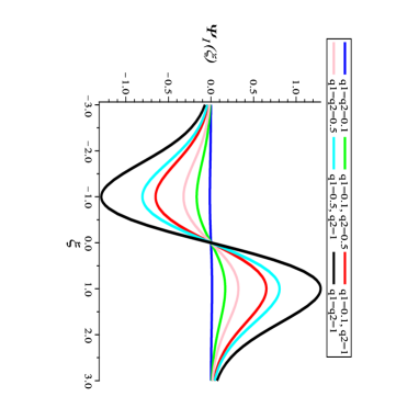
Figure 1: Stationary state $\Psi_{1}$ for several $(q_{1},q_{2})$ parameters. The undeformed case is $q_{1}=1$ and $q_{2}\to 1$ (black curve) and the most deformed case is $q_{1}=q_{2}=0.1$ (blue curve).

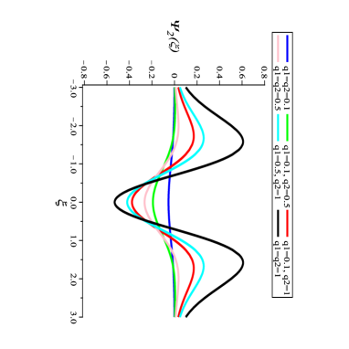
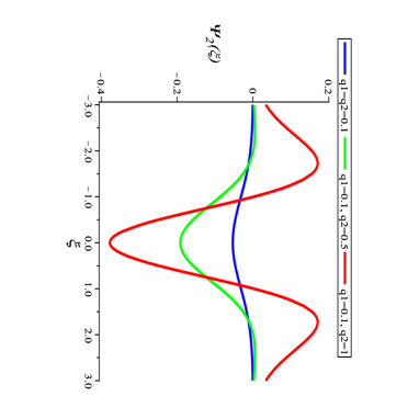
Figure 2: Stationary state $\Psi_{2}$ for several $(q_{1},q_{2})$ parameters. The undeformed case is $q_{1}=1$ and $q_{2}\to 1$ (black curve) and the most deformed case is $q_{1}=q_{2}=0.1$ (blue curve).

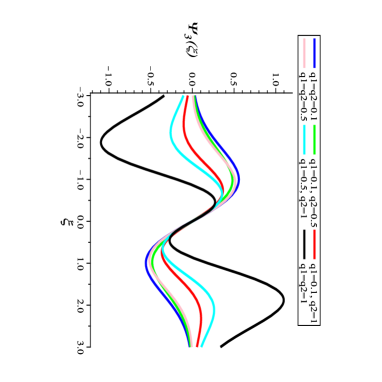
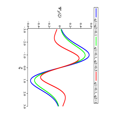
Figure 3: Stationary state $\Psi_{3}$ for several $(q_{1},q_{2})$ parameters. The undeformed case is $q_{1}=1$ and $q_{2}\to 1$ (black curve) and the most deformed case is $q_{1}=q_{2}=0.1$ (blue curve).

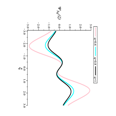
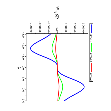
Figure 4: Stationary state $\Psi_{3q}$ for several $(q)$ parameter. The undeformed case is $q=1$ (black curve) and the most deformed case is $q_{=}0.1$ (blue curve).

We can observe in the Figs. 1-3 that the behavior of the curves is altered with the presence of the ($q_{1},q_{2}$)-deformation. In all cases the black curves do not present deformation, since they are in the limit $q_{1}=1$ and $q_{2}\to 1$ (or vice versa) and the most deformed case is $q_{1}=q_{2}=0.1$ depicted by the blue curves. In Fig. 1 we can observe that the behaviors are similar.

The deformation acts simply varying the amplitude of the curves and by shifting the positions of nodes of wave functions.

In Figs. 2 and 3 we note that the presence of the deformation develops a greater role in the next excited states. The behavior of the other curves become very different from the black curve. On the right panel we have a zoom in three curves to carry it out a better analysis of the deformation. It is worth mentioning that the number of nodes of wave function decreases significantly (by a factor of 2) as the deformation becomes strong enough. This means that in this limit the states are maintained to be even or odd states, but developing less excited modes. As we have anticipated in bri1 , we can interpret the deformation parameters as impurity (or disorder) factors since the $q$-deformation affects the oscillator frequency, which in turn may be associated with the changing of the number of nodes. For further discussion of this phenomenon in deformed diamagnetic material see bri1 — and also gsr for experimental results.

Damaskinsky and Kulish obtained the $q$-Hermite polynomials dam . We can make a little discussion about our results in connection with $q$-oscillators by reducing the pair $(q_{1},q_{2})$ to just $q$ as shown in Eq. (14). Now, we plot in Fig. 4 the wave function $\Psi_{3q}$ for some values of $q$. Notice that differently from the $(q_{1},q_{2})$ case as one increases the deformation only the peak amplitudes change. This behavior reinforce the fact that $(q_{1},q_{2})$-deformation develops a more rich physical behavior.

IV Conclusions

As expected from Eq.(49), the Fibonacci oscillators have modified behavior in the stationary states. It is clear that as the deformation parameters decrease in relation to the undeformed case $q_{1}=1$ and $q_{2}\to 1$ (or vice versa), the distinct behavior of the curves becomes more evident. This also becomes clear as we look at the Hermite polynomials (50) where $H_{3}$ feels a greater presence of $q_{1}$ and $q_{2}$ than $H_{1}$. We can conclude that the more the states are excited the more strong is the deformation on them. This may find interesting applications in quantum mechanics such as inclusion of disorders and impurities in the quantum system. For instance, in bri several studies were put forward uncovering the fact that the $q$-deformation affects the oscillator frequency which may be associated with the changing in the strength of the ‘spring constant’ associated with such an oscillator as a consequence of introduction of impurities or disorders in the system. This should be further addressed elsewhere.

References

- (1) J.J. Sakurai, Modern Quantum Mechanics, (Late-Univ. of California, LA (1985)).
- (2) David J. Griffiths, Introduction to Quantum Mechanics, (Pearson Prentice Hall, USA (2005)).
- (3) A. Lavagno, P.N. Swamy, Phys. Rev. E 65, 036101 (2002). A. Lavagno, P.N. Swamy, Found Phys. 40, 814-828 (2010).
- (4) R. Hinterding, J. Wess, Eur. Phys. J. C 6, 183-186 (1999).
- (5) Ö.F. Dayi, I.H. Duru, Int. J. Mod. Phys. A 12, 2373 (1997).
- (6) A.R. Plastino, A.M.C. Souza, F.D. Nobre and C. Tsallis, Phys. Rev. A 90, 062134 (2014).
- (7) O.K. Pashaev, arXiv:math-ph/1411.4514v1.
- (8) M. Micu, J. Phys. A: Math Gen. 32, 7765-7777 (1999).
- (9) C.R. Lee, Chinese J. Phys. 28, 381-385 (1990).
- (10) A. Lorek, A. Ruffing and J. Wess, Z. Phys. C 74, 369-378 (1997).
- (11) M. S. Abdalla and H. Eleuch, J. Appl. Phys. 115, 234906 (2014).
- (12) M. Chaichian, R. Gonzales Felipe, C. Montonen, J. Phys. A: Math. Gen. 26, 4017 (1993).
- (13) A. Lavagno, G. Gervino, J. Phys. Conf. Series 174, 012071 (2009).
- (14) Y.J. Ng, J. Phys. A 23, 1023 (1990).
- (15) B. Mirza, H. Mohammadzadeh, J. Phys. A: Math. Theor. 44, 475003 (2011).
- (16) F.H. Jackson, Proc. Edin. Math. Soc. 22, 28-39(1904); F.H. Jackson, Mess. Math. 38, 57 (1909).
- (17) E.G. Floratos, J. Phys. Math. 24, 4739 (1991).
- (18) M. Arik, D.D. Coon, J. Math. Phys. 17, 524 (1976); M. Arik, et al., Z. Phys. C 55, 89-95 (1992).
- (19) R. Chakrabarti, R. Jagannathan, J. Phys. A: Math. Gen. 24, L711 (1991).
- (20) W.S. Chung et al., Phys. Lett. A 183, 363 (1993).
- (21) S.S. Mizrahi, J.P. Camargo Lima, V.V. Dodonov, J. Phys. A 37, 3707 (2004).
- (22) I.M. Burban, Phys. Lett. A 366, 308 (2007).
- (23) A. Algin, Phys. Lett. A 292, 251-255 (2002); A. Algin, B. Deviren, J. Phys. A: Math. Gen. 38, 5945-5956 (2005); A. Algin, J. Stat. Mech. Theor. Exp. P10009, 10 (2008); A. Algin, J. Stat. Mech. Theor. Exp. P04007, 04 (2009); A. Algin, J. CNSNS 15, 1372-1377 (2010).
- (24) J.D. Bukweli Kyemba, M. Hounkonnou, J. Phys. A 45, 225204 (2012).
- (25) A.M. Gavrilik, A.P. Rebesh, Mod. Phys. Lett. A 22, 949-960 (2007); A.M. Gavrilik, I.I. Kachurik, A.P. Rebesh, J. Phys. A 43, 24, 245204 (2010); A.M. Gavrilik, A.P. Rebesh, Eur. Phys. J.A 47, 55 (2011); A.P. Rebesh, I.I. Kachurik, A.M. Gavrilik, Ukr. J. Phys. 58, n. 12 (2013); A.M. Gavrilik, I.I. Kachurik, A.P. Rebesh, arXiv:cond-mat.stat-mech/1309.1363v1; A.M. Gavrilik et al., arXiv:cond-mat.stat-mech/1709.05931v2; A.M. Gavrilik et al., Phys. A: Stat. Mech. & its Applic. 506, 835-843 (2018).
- (26) A.A. Marinho, F.A. Brito, C. Chesman, Physica A 411, 74-79 (2014); A.A. Marinho, F.A. Brito, C. Chesman, J. Phys. Conf. Series 568, 012009 (2014); A.A. Marinho, F.A. Brito, C. Chesman, Physica A 443, 324-332 (2016).
- (27) L. Biedenharn, J. Phys. A: Math. Gen. 22, L873 (1989).
- (28) A. Macfarlane, J. Phys. A: Math. Gen. 22, 4581 (1989).
- (29) J. Fuchs, Affine Lie Algebras and Quantum Groups, Cambridge University Press (1992).
- (30) A. Erzan, Phys. Lett. A 225, 235 (1997).
- (31) V.V. Borzov, E.V. Damaskinsky, Zap. Nauchn. Sem. PDMI 308, 48-66 (2004) and arXiv:quant-ph/0407252v1; V.V. Borzov, E.V. Damaskinsky, J. Math. Sci. 136, 3564-3579 (2006).
- (32) Daoud M., Kibler M., Phys. Lett A 206, 13-17 (1995).
- (33) Gong R. S., Phys. Lett A 199, 81-85 (1995).
- (34) H. Exton, -Hypergeometric Functions and Applications, John Wiley and Sons, New York, (1983).
- (35) G. Gasper, M. Rahman, Basic Hypergeometric Functions, Cambridge Univ. Press, Cambridge, (1991).
- (36) T. Ernst, The History of -calculus and a new method. (Dep. Math., Uppsala Univ. 1999-2000).
- (37) D. Bonatsos, C. Daskaloyannis, Prog. Part. Nuc. Phys. 43, 537-618 (1999).
- (38) V. Kac, P. Cheung, Quantum Calculus, (Universitext, Springer-verlag), (2002).
- (39) I.M. Burban, A.U. Klimyk, Lett. Math. Phys. 29, 13-18 (1993); I.M. Burban, A.U. Klimyk, Integral Transforms and Special Functions 2, 15-36 (1994).
- (40) E.V. Damaskinsky, P. Kulish, Zap. Nauchn. Sem. LOMI 199, 81-90 (1992) and English version J. Math. Sci. 77, 3069-3075 (1995).
- (41) T.S. Chihara, An Introduction to Orthogonal Polynomials, (Gordon and Breach (1978)).
- (42) F.A. Brito, A.A. Marinho, Physica A 390, 2497-2503 (2011).
- (43) G. Srinivas, et al., J. Mater. Chem. 19, 5239-5243 (2009); G. Srinivas, et al., Phys. Chem. Chem. Phys. 33, 758-761 (2010).