Post-Specialisation: Retrofitting Vectors of Words
Unseen in Lexical Resources

Abstract

Word vector specialisation (also known as retrofitting) is a portable, light-weight approach to fine-tuning arbitrary distributional word vector spaces by injecting external knowledge from rich lexical resources such as WordNet. By design, these post-processing methods only update the vectors of words occurring in external lexicons, leaving the representations of all unseen words intact. In this paper, we show that constraint-driven vector space specialisation can be extended to unseen words. We propose a novel post-specialisation method that: a) preserves the useful linguistic knowledge for seen words; while b) propagating this external signal to unseen words in order to improve their vector representations as well. Our post-specialisation approach explicits a non-linear specialisation function in the form of a deep neural network by learning to predict specialised vectors from their original distributional counterparts. The learned function is then used to specialise vectors of unseen words. This approach, applicable to any post-processing model, yields considerable gains over the initial specialisation models both in intrinsic word similarity tasks, and in two downstream tasks: dialogue state tracking and lexical text simplification. The positive effects persist across three languages, demonstrating the importance of specialising the full vocabulary of distributional word vector spaces.

1 Introduction

Word representation learning is a key research area in current Natural Language Processing (NLP), with its usefulness demonstrated across a range of tasks Collobert et al. (2011); Chen and Manning (2014); Melamud et al. (2016b). The standard techniques for inducing distributed word representations are grounded in the distributional hypothesis Harris (1954): they rely on co-occurrence information in large textual corpora Mikolov et al. (2013b); Pennington et al. (2014); Levy and Goldberg (2014); Levy et al. (2015); Bojanowski et al. (2017). As a result, these models tend to coalesce the notions of semantic similarity and (broader) conceptual relatedness, and cannot accurately distinguish antonyms from synonyms Hill et al. (2015); Schwartz et al. (2015). Recently, we have witnessed a rise of interest in representation models that move beyond stand-alone unsupervised learning: they leverage external knowledge in human- and automatically-constructed lexical resources to enrich the semantic content of distributional word vectors, in a process termed semantic specialisation.

This is often done as a post-processing (sometimes referred to as retrofitting) step: input word vectors are fine-tuned to satisfy linguistic constraints extracted from lexical resources such as WordNet or BabelNet Faruqui et al. (2015); Mrkšić et al. (2017). The use of external curated knowledge yields improved word vectors for the benefit of downstream applications Faruqui (2016). At the same time, this specialisation of the distributional space distinguishes between true similarity and relatedness, and supports language understanding tasks Kiela et al. (2015); Mrkšić et al. (2017).

While there is consensus regarding their benefits and ease of use, one property of the post-processing specialisation methods slips under the radar: most existing post-processors update word embeddings only for words which are present (i.e., seen) in the external constraints, while vectors of all other (i.e., unseen) words remain unaffected. In this work, we propose a new approach that extends the specialisation framework to unseen words, relying on the transformation of the vector (sub)space of seen words. Our intuition is that the process of fine-tuning seen words provides implicit information on how to leverage the external knowledge to unseen words. The method should preserve the already injected knowledge for seen words, simultaneously propagating the external signal to unseen words in order to improve their vectors.

The proposed post-specialisation method can be seen as a two-step process, illustrated in Fig. 1(a): 1) We use a state-of-the-art specialisation model to transform the subspace of seen words from the input distributional space into the specialised subspace; 2) We learn a mapping function based on the transformation of the “seen subspace”, and then apply it to the distributional subspace of unseen words. We allow the proposed post-specialisation model to learn from large external linguistic resources by implementing the mapping as a deep feed-forward neural network with non-linear activations. This allows the model to learn the generalisation of the fine-tuning steps taken by the initial specialisation model, itself based on a very large number (e.g., hundreds of thousands) of external linguistic constraints.

As indicated by the results on word similarity and two downstream tasks (dialogue state tracking and lexical text simplification) our post-specialisation method consistently outperforms state-of-the-art methods which specialise seen words only. We report improvements using three distinct input vector spaces for English and for three test languages (English, German, Italian), verifying the robustness of our approach.

2 Related Work and Motivation

Vector Space Specialisation

A standard approach to incorporating external and background knowledge into word vector spaces is to pull the representations of similar words closer together and to push words in undesirable relations (e.g., antonyms) away from each other. Some models integrate such constraints into the training procedure and jointly optimize distributional and non-distributional objectives: they modify the prior or the regularisation Yu and Dredze (2014); Xu et al. (2014); Bian et al. (2014); Kiela et al. (2015), or use a variant of the SGNS-style objective Liu et al. (2015); Ono et al. (2015); Osborne et al. (2016); Nguyen et al. (2017). In theory, word embeddings obtained by these joint models could be as good as representations produced by models which fine-tune input vector space. However, their performance falls behind that of fine-tuning methods Wieting et al. (2015). Another disadvantage is that their architecture is tied to a specific underlying model (typically word2vec models).

In contrast, fine-tuning models inject external knowledge from available lexical resources (e.g., WordNet, PPDB) into pre-trained word vectors as a post-processing step Faruqui et al. (2015); Rothe and Schütze (2015); Wieting et al. (2015); Nguyen et al. (2016); Mrkšić et al. (2016); Cotterell et al. (2016); Mrkšić et al. (2017). Such post-processing models are popular because they offer a portable, flexible, and light-weight approach to incorporating external knowledge into arbitrary vector spaces, yielding state-of-the-art results on language understanding tasks Faruqui et al. (2015); Mrkšić et al. (2016); Kim et al. (2016); Vulić et al. (2017b).

Existing post-processing models, however, suffer from a major limitation. Their modus operandi is to enrich the distributional information with external knowledge only if such knowledge is present in a lexical resource. This means that they update and improve only representations of words actually seen in external resources. Because such words constitute only a fraction of the whole vocabulary (see Sect. 4), most words, unseen in the constraints, retain their original vectors. The main goal of this work is to address this shortcoming by specialising all words from the initial distributional space.

3 Methodology: Post-Specialisation

Our starting point is the state-of-the-art specialisation model attract-repel (ar) Mrkšić et al. (2017), outlined in Sect. 3.1. We opt for the ar model due to its strong performance and ease of use, but we note that the proposed post-specialisation approach for specialising unseen words, described in Sect. 3.2, is applicable to any post-processor, as empirically validated in Sect. 5.

3.1 Initial Specialisation Model: ar

Let $\mathcal{V}_{s}$ be the vocabulary, $A$ the set of synonymous attract word pairs (e.g., rich and wealthy), and $R$ the set of antonymous repel word pairs (e.g., increase and decrease). The attract-repel procedure operates over mini-batches of such pairs $\mathcal{B}_{A}$ and $\mathcal{B}_{R}$. Let each word pair $(x_{l},x_{r})$ in these sets correspond to a vector pair $(\mathbf{x}_{l},\mathbf{x}_{r})$. A mini-batch of $b_{att}$ attract word pairs is given by $\mathcal{B}_{A}=[(\mathbf{x}_{l}^{1},\mathbf{x}_{r}^{1}),\ldots,(\mathbf{x}_{l}^{k_{1}},\mathbf{x}_{r}^{k_{1}})]$ (analogously for $\mathcal{B}_{R}$, which consists of $b_{rep}$ pairs).

Next, the sets of negative examples $T_{A}=[(\mathbf{t}_{l}^{1},\mathbf{t}_{r}^{1}),\ldots,(\mathbf{t}_{l}^{k_{1}},\mathbf{t}_{r}^{k_{1}})]$ and $T_{R}=[(\mathbf{t}_{l}^{1},\mathbf{t}_{r}^{1}),\ldots,(\mathbf{t}_{l}^{k_{2}},\mathbf{t}_{r}^{k_{2}})]$ are defined as pairs of negative examples for each $A$ and $R$ pair in mini-batches $\mathcal{B}_{A}$ and $\mathcal{B}_{R}$. These negative examples are chosen from the word vectors present in $\mathcal{B}_{A}$ or $\mathcal{B}_{R}$ so that, for each $A$ pair $(\mathbf{x}_{l},\mathbf{x}_{r})$, the negative example pair $(\mathbf{t}_{l},\mathbf{t}_{r})$ is chosen so that $\mathbf{t}_{l}$ is the vector closest (in terms of cosine distance) to $\mathbf{x}_{l}$ and $\mathbf{t}_{r}$ is closest to $\mathbf{x}_{r}$. The negatives are used 1) to force $A$ pairs to be closer to each other than to their respective negative examples; and 2) to force $R$ pairs to be further away from each other than from their negative examples. The first term of the cost function pulls $A$ pairs together:

$$Att(\mathcal{B}_{A},T_{A})\leavevmode\nobreak\ =\sum_{i=1}^{b_{att}} \big{[}\leavevmode\nobreak\ \tau\left(\delta_{att}+\mathbf{x}_{l}^{i}\mathbf{t}_{l}^{i}-\mathbf{x}_{l}^{i}\mathbf{x}_{r}^{i}\right)$$

$$+ \tau\left(\delta_{att}+\mathbf{x}_{r}^{i}\mathbf{t}_{r}^{i}-\mathbf{x}_{l}^{i}\mathbf{x}_{r}^{i}\right)\big{]}$$ (1)

where $\tau(z)=\max(0,z)$ is the standard rectifier function Nair and Hinton (2010) and $\delta_{att}$ is the attract margin: it determines how much closer these vectors should be to each other than to their respective negative examples. The second, repel term in the cost function is analogous: it pushes $R$ word pairs away from each other by the margin $\delta_{rep}$.

Finally, in addition to the $A$ and $R$ terms, a regularisation term is used to preserve the semantic content originally present in the distributional vector space, as long as this information does not contradict the injected external knowledge. Let $\mathcal{V}(\mathcal{B})$ be the set of all word vectors present in a mini-batch, the distributional regularisation term is then:

$$Reg(\mathcal{B}_{A},\mathcal{B}_{R})=\sum\limits_{\mathbf{x}_{i}\in V(\mathcal{B}_{A}\cup\mathcal{B}_{R})}\lambda_{reg}\left\|\widehat{\mathbf{x}_{i}}-\mathbf{x}_{i}\right\|_{2}$$ (2)

where $\lambda_{reg}$ is the $L_{2}$-regularisation constant and $\widehat{\mathbf{x}_{i}}$ denotes the original (distributional) word vector for word $x_{i}$. The full attract-repel cost function is finally constructed as the sum of all three terms.

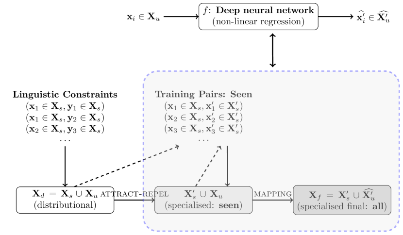
(a) High-level illustration

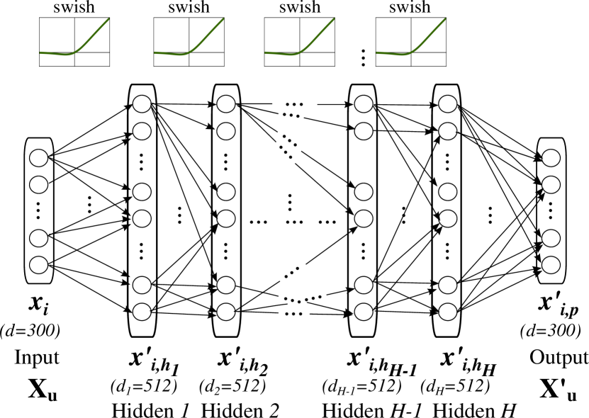
(b) Low-level implementation: deep feed-forward neural network

Figure 1: (a) High-level illustration of the post-specialisation approach: the subspace $\mathbf{X}_{s}$ of the initial distributional vector space $\mathbf{X}_{d}=\mathbf{X}_{s}\cup\mathbf{X}_{u}$ is first specialised/fine-tuned by the attract-repel specialisation model (or any other post-processing model) to obtain the transformed subspace $\mathbf{X}^{\prime}_{s}$. The words present (i.e., seen) in the input set of linguistic constraints are now assigned different representations in $\mathbf{X}_{s}$ (the original distributional vector) and $\mathbf{X}^{\prime}_{s}$ (the specialised vector): they are therefore used as training examples to learn a non-linear cross-space mapping function. This function is then applied to all word vectors $\mathbf{x}_{i}\in\mathbf{X}_{u}$ representing words unseen in the constraints to yield a specialised subspace $\widehat{\mathbf{X}^{\prime}_{u}}$. The final space is $\mathbf{X}_{f}=\mathbf{X}^{\prime}_{s}\cup\widehat{\mathbf{X}^{\prime}_{u}}$, and it contains transformed representations for all words from the initial space $\mathbf{X}_{d}$. (b) The actual implementation of the non-linear regression function which maps from $\mathbf{X}_{u}$ to $\widehat{\mathbf{X}^{\prime}_{u}}$: a deep feed-forward fully-connected neural net with non-linearities and $H$ hidden layers.

3.2 Specialisation of Unseen Words

Problem Formulation

The goal is to learn a global transformation function that generalises the perturbations of the initial vector space made by attract-repel (or any other specialisation procedure), as conditioned on the external constraints. The learned function propagates the signal coded in the input constraints to all the words unseen during the specialisation process. We seek a regression function $f:\mathbb{R}^{dim}\rightarrow\mathbb{R}^{dim}$, where $dim$ is the vector space dimensionality. It maps word vectors from the initial vector space $\mathbf{X}$ to the specialised target space $\mathbf{X}^{\prime}$. Let $\widehat{\mathbf{X}^{\prime}}=f(\mathbf{X})$ refer to the predicted mapping of the vector space, while the mapping of a single word vector is denoted $\widehat{\mathbf{x}^{\prime}_{i}}=f(\mathbf{x}_{i})$.

An input distributional vector space $\mathbf{X}_{d}$ represents words from a vocabulary $\mathcal{V}_{d}$. $\mathcal{V}_{d}$ may be divided into two vocabulary subsets: $\mathcal{V}_{d}=\mathcal{V}_{s}\cup\mathcal{V}_{u}$, $\mathcal{V}_{s}\cap\mathcal{V}_{u}=\emptyset$, with the accompanying vector subspaces $\mathbf{X}_{d}=\mathbf{X}_{s}\sqcup\mathbf{X}_{u}$. $\mathcal{V}_{s}$ refers to the vocabulary of seen words: those that appear in the external linguistic constraints and have their embeddings changed in the specialisation process. $\mathcal{V}_{u}$ denotes the vocabulary of unseen words: those not present in the constraints and whose embeddings are unaffected by the specialisation procedure.

The ar specialisation process transforms only the subspace $\mathbf{X}_{s}$ into the specialised subspace $\mathbf{X}^{\prime}_{s}$. All words $x_{i}\in\mathcal{V}_{s}$ may now be used as training examples for learning the explicit mapping function $f$ from $\mathbf{X}_{s}$ into $\mathbf{X}^{\prime}_{s}$. If $N=|\mathcal{V}_{s}|$, we in fact rely on $N$ training pairs: $(\mathbf{x}_{i},\mathbf{x}^{\prime}_{i})=\{\mathbf{x}_{i}\in\mathbf{X}_{s},\mathbf{x}^{\prime}_{i}\in\mathbf{X}^{\prime}_{s}\}$. Function $f$ can then be applied to unseen words $x\in\mathcal{V}_{u}$ to yield the specialised subspace $\widehat{\mathbf{X}^{\prime}_{u}}=f(\mathbf{X}_{u})$. The specialised space containing all words is then $\mathbf{X}_{f}=\mathbf{X}^{\prime}_{s}\cup\widehat{\mathbf{X}^{\prime}_{u}}$. The complete high-level post-specialisation procedure is outlined in Fig. 1(a).

Note that another variant of the approach could obtain $\mathbf{X}_{f}$ as $\mathbf{X}_{f}=f(\mathbf{X}_{d})$, that is, the entire distributional space is transformed by $f$. However, this variant seems counter-intuitive as it forgets the actual output of the initial specialisation procedure and replaces word vectors from $\mathbf{X}^{\prime}_{s}$ with their approximations, i.e., $f$-mapped vectors.

Objective Functions

As mentioned, the $N$ seen words $x_{i}\in\mathcal{V}_{s}$ in fact serve as our “pseudo-translation” pairs supporting the learning of a cross-space mapping function. In practice, in its high-level formulation, our mapping problem is equivalent to those encountered in the literature on cross-lingual word embeddings where the goal is to learn a shared cross-lingual space given monolingual vector spaces in two languages and $N_{1}$ translation pairs Mikolov et al. (2013a); Lazaridou et al. (2015); Vulić and Korhonen (2016b); Artetxe et al. (2016, 2017); Conneau et al. (2017); Ruder et al. (2017). In our setup, the standard objective based on $L_{2}$-penalised least squares may be formulated as follows:

$$f_{\textsc{mse}}=\text{arg min}||f(\mathbf{X}_{s})-\mathbf{X}^{\prime}_{s}||^{2}_{F}$$ (3)

where $||\cdot||_{F}^{2}$ denotes the squared Frobenius norm. In the most common form $f(\mathbf{X}_{s})$ is simply a linear map/matrix $\mathbf{W}_{f}\in\mathbb{R}^{dim\times dim}$ Mikolov et al. (2013a) as follows: $f(\mathbf{X})=\mathbf{W}_{f}\mathbf{X}$.

After learning $f$ based on the $\mathbf{X}_{s}\rightarrow\mathbf{X}^{\prime}_{s}$ transformation, one can simply apply $f$ to unseen words: $\widehat{\mathbf{X}^{\prime}_{u}}=f(\mathbf{X}_{u})$. This linear mapping model, termed linear-mse, has an analytical solution Artetxe et al. (2016), and has been proven to work well with cross-lingual embeddings. However, given that the specialisation model injects hundreds of thousands (or even millions) of linguistic constraints into the distributional space (see later in Sect. 4), we suspect that the assumption of linearity is too limiting and does not fully hold in this particular setup.

Using the same $L_{2}$-penalized least squares objective, we can thus replace the linear map with a non-linear function $f:\mathbb{R}^{dim}\rightarrow\mathbb{R}^{dim}$. The non-linear mapping, illustrated by Fig. 1(b), is implemented as a deep feed-forward fully-connected neural network (DFFN) with $H$ hidden layers and non-linear activations. This variant is called nonlinear-mse.

Another variant objective is the contrastive margin-based ranking loss with negative sampling (mm) similar to the original attract-repel objective, used in other applications in prior work (e.g., for cross-modal mapping) Weston et al. (2011); Frome et al. (2013); Lazaridou et al. (2015); Kummerfeld et al. (2015). Let $\widehat{\mathbf{x^{\prime}}_{i}}=f(\mathbf{x_{i}})$ denote the predicted vector for the word $x_{i}\in\mathcal{V}_{s}$, and let $\mathbf{x^{\prime}}_{i}$ refer to the “true” vector of $x_{i}$ in the specialised space $\mathbf{X}^{\prime}_{s}$ after the ar specialisation procedure. The mm loss is then defined as follows:

$$J_{\textsc{MM}}=\sum_{i=1}^{N}\sum_{j\neq i}^{k}\tau\Big{(}\delta_{mm}-cos\big{(}\widehat{\mathbf{x^{\prime}}_{i}},\mathbf{x^{\prime}}_{i}\big{)}+cos\big{(}\widehat{\mathbf{x^{\prime}}_{i}},\mathbf{x^{\prime}}_{j}\big{)}\Big{)}$$

where $cos$ is the cosine similarity measure, $\delta_{mm}$ is the margin, and $k$ is the number of negative samples. The objective tries to learn the mapping $f$ so that each predicted vector $\widehat{\mathbf{x^{\prime}}_{i}}$ is by the specified margin $\delta_{mm}$ closer to the correct target vector $\mathbf{x^{\prime}}_{i}$ than to any other of $k$ target vectors $\mathbf{x^{\prime}}_{j}$ serving as negative examples. Function $f$ can again be either a simple linear map (linear-mm), or implemented as a DFFN (nonlinear-mm, see Fig. 1(b)).

4 Experimental Setup

Starting Word Embeddings ($\mathbf{X}_{d}=\mathbf{X}_{s}\cup\mathbf{X}_{u}$) To test the robustness of our approach, we experiment with three well-known, publicly available collections of English word vectors: 1) Skip-Gram with Negative Sampling (sgns-bow2) Mikolov et al. (2013b) trained on the Polyglot Wikipedia Al-Rfou et al. (2013) by Levy and Goldberg (2014) using bag-of-words windows of size 2; 2) glove Common Crawl Pennington et al. (2014); and 3) fastText Bojanowski et al. (2017), a SGNS variant which builds word vectors as the sum of their constituent character n-gram vectors. All word embeddings are $300$-dimensional.

AR Specialisation and Constraints ($\mathbf{X}_{s}\rightarrow\mathbf{X}^{\prime}_{s}$)

We experiment with linguistic constraints used before by Mrkšić et al. (2017); Vulić et al. (2017a): they extracted monolingual synonymy/attract pairs from the Paraphrase Database (PPDB) Ganitkevitch et al. (2013); Pavlick et al. (2015) (640,435 synonymy pairs in total), while their antonymy/repel constraints came from BabelNet Navigli and Ponzetto (2012) (11,939 pairs).

The coverage of $\mathcal{V}_{d}$ vocabulary words in the constraints illustrates well the problem of unseen words with the fine-tuning specialisation models. For instance, the constraints cover only a small subset of the entire vocabulary $\mathcal{V}_{d}$ for sgns-bow2: 16.6%. They also cover only 15.3% of the top 200K most frequent $\mathcal{V}_{d}$ words from fastText.

Network Design and Parameters ($\mathbf{X}_{u}\rightarrow\widehat{\mathbf{X}^{\prime}_{u}}$)

The non-linear regression function $f:\mathbb{R}^{d}\rightarrow\mathbb{R}^{d}$ is a DFFN with $H$ hidden layers, each of dimensionality $d_{1}=d_{2}=\ldots=d_{H}=512$ (see Fig. 1(b)). Non-linear activations are used in each layer and omitted only before the final output layer to enable full-range predictions (see Fig. 1(b) again).

The choices of non-linear activation and initialisation are guided by recent recommendations from the literature. First, we use swish Ramachandran et al. (2017); Elfwing et al. (2017) as non-linearity, defined as $swish(x)=x\cdot\text{sigmoid}(\beta x)$. We fix $\beta=1$ as suggested by Ramachandran et al. (2017). Second, we use the he normal initialisation He et al. (2015), which is preferred over the xavier initialisation Glorot and Bengio (2010) for deep models Mishkin and Matas (2016); Li et al. (2016), although in our experiments we do not observe a significant difference in performance between the two alternatives. We set $H=5$ in all experiments without any fine-tuning; we also analyse the impact of the network depth in Sect. 5.

Optimisation

For the ar specialisation step, we adopt the original suggested model setup. Hyperparameter values are set to: $\delta_{att}=0.6$, $\delta_{rep}=0.0$, $\lambda_{reg}=10^{-9}$ Mrkšić et al. (2017). The models are trained for 5 epochs with Adagrad Duchi et al. (2011), with batch sizes set to $b_{att}=b_{rep}=50$, again as in the original work.

For training the non-linear mapping with DFFN (Fig. 1(b)), we use the Adam algorithm Kingma and Ba (2015) with default settings. The model is trained for 100 epochs with early stopping on a validation set. We reserve 10% of all available seen data (i.e., the words from $\mathcal{V}_{s}$ represented in $\mathbf{X}_{s}$ and $\mathbf{X}^{\prime}_{s}$) for validation, the rest are used for training. For the mm objective, we set $\delta_{mm}=0.6$ and $k=25$ in all experiments without any fine-tuning.

5 Results and Discussion

	Setup: hold-out						Setup: all
	glove		sgns-bow2		fastText		glove		sgns-bow2		fastText
	SL	SV	SL	SV	SL	SV	SL	SV	SL	SV	SL	SV
Distributional: $\mathbf{X}_{d}$	.408	.286	.414	.275	.383	.255	.408	.286	.414	.275	.383	.255
+ar specialisation: $\mathbf{X}^{\prime}_{s}$	.408	.286	.414	.275	.383	.255	.690	.578	.658	.544	.629	.502
++Mapping unseen: $\mathbf{X}_{f}$
linear-mse	.504	.384	.447	.309	.405	.285	.690	.578	.656	.551	.628	.502
nonlinear-mse	.549	.407	.484	.344	.459	.329	.694	.586	.663	.556	.631	.506
linear-mm	.548	.422	.468	.329	.419	.308	.697	.582	.663	.554	.628	.487
nonlinear-mm	.603	.480	.531	.391	.471	.349	.705	.600	.667	.562	.638	.507

Table 1: Spearman’s $\rho$ correlation scores for three word vector collections on two English word similarity datasets, SimLex-999 (SL) and SimVerb-3500 (SV), using different mapping variants, evaluation protocols, and word vector spaces: from the initial distributional space $\mathbf{X}_{d}$ to the fully specialised space $\mathbf{X}_{f}$. $H=5$.

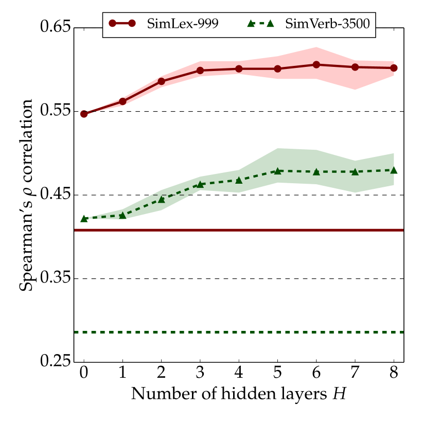
(a) glove

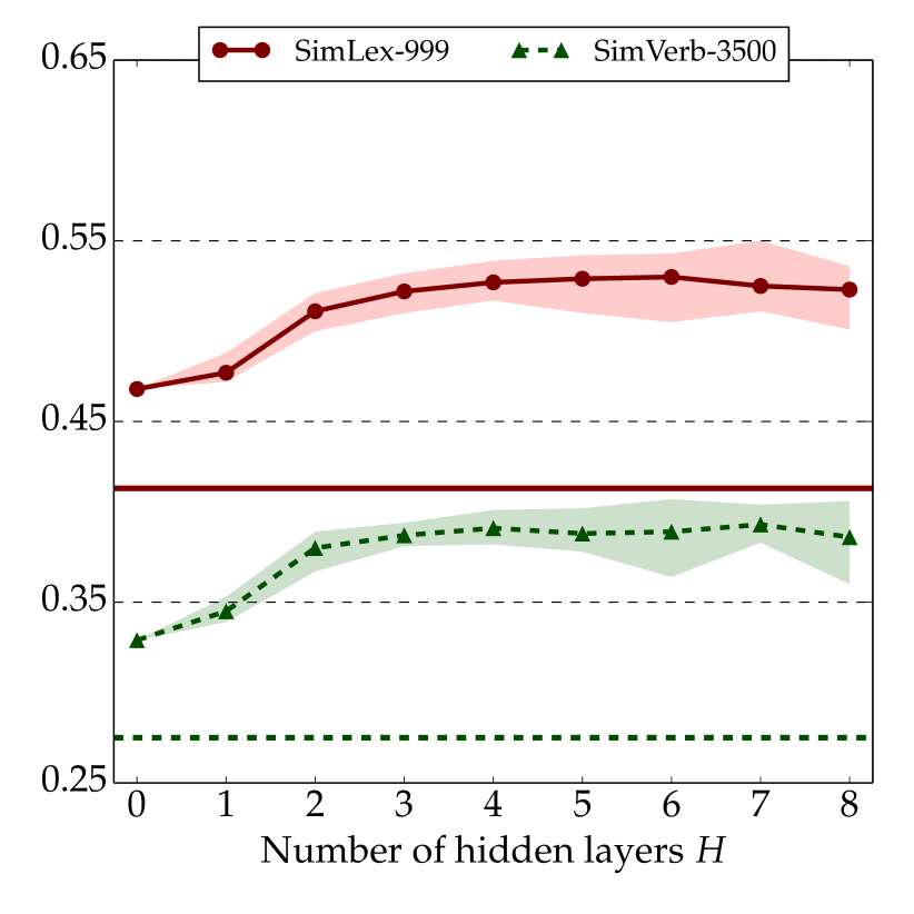
(b) sgns-bow2

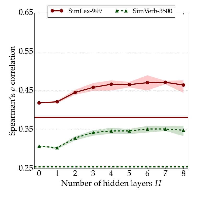
(c) fastText

Figure 2: The results of the hold-out experiments on SimLex-999 and SimVerb-3500 after applying our non-linear vector space transformation with different depths (hidden layer size $H$, see Fig. 1(b)). The results are presented as averages over 20 runs with the nonlinear-mm variant, the shaded regions are spanned by the maximum and minimum scores obtained. Thick horizontal lines refer to Spearman’s rank correlations achieved in the initial space $\mathbf{X}_{d}$. $H=0$ denotes the standard linear regression model Mikolov et al. (2013a); Lazaridou et al. (2015) (linear-mm shown since it outperforms linear-mse).

5.1 Intrinsic Evaluation: Word Similarity

Evaluation Protocol

The first set of experiments evaluates vector spaces with different specialisation procedures intrinsically on word similarity benchmarks: we use the SimLex-999 dataset Hill et al. (2015), and SimVerb-3500 Gerz et al. (2016), a recent verb pair similarity dataset providing similarity ratings for 3,500 verb pairs. Spearman’s $\rho$ rank correlation is used as the evaluation metric.

We evaluate word vectors in two settings. First, in a synthetic hold-out setting, we remove all linguistic constraints which contain words from the SimLex and SimVerb evaluation data, effectively forcing all SimLex and SimVerb words to be unseen by the ar specialisation model. The specialised vectors for these words are estimated by the learned non-linear DFFN mapping model. Second, the all setting is a standard “real-life” scenario where some test (SimLex/SimVerb) words do occur in the constraints, while the mapping is learned for the remaining words.

Results and Analysis

The results with the three word vector collections are provided in Tab. 1. In addition, Fig. 2 plots the influence of the network depth $H$ on the model’s performance.

The results suggest that the mapping of unseen words is universally useful, as the highest correlation scores are obtained with the final fully specialised vector space $\mathbf{X}_{f}$ for all three input spaces. The results in the hold-out setup are particularly indicative of the improvement achieved by our post-specialisation method. For instance, it achieves a +0.2 correlation gain with glove on both SimLex and SimVerb by specialising vector representations for words present in these datasets without seeing a single external constraint which contains any of these words. This suggests that the perturbation of the seen subspace $\mathbf{X}_{s}$ by attract-repel contains implicit knowledge that can be propagated to $\mathbf{X}_{u}$, learning better representations for unseen words. We observe small but consistent improvements across the board in the all setup. The smaller gains can be explained by the fact that a majority of SimLex and SimVerb words are present in the external constraints (93.7% and 87.2%, respectively).

The scores also indicate that both non-linearity and the chosen objective function contribute to the quality of the learned mapping: largest gains are reported with the nonlinear-mm variant which a) employs non-linear activations and b) replaces the basic mean-squared-error objective with max-margin. The usefulness of the latter has been established in prior work on cross-space mapping learning Lazaridou et al. (2015). The former indicates that the initial ar transformation is non-linear. It is guided by a large number of constraints; their effect cannot be captured by a simple linear map as in prior work on, e.g., cross-lingual word embeddings Mikolov et al. (2013a); Ruder et al. (2017).

Finally, the analysis of the network depth $H$ indicates that going deeper helps only to a certain extent. Adding more layers allows for a richer parametrisation of the network (which is beneficial given the number of linguistic constraints used by ar). This makes the model more expressive, but it seems to saturate with larger $H$ values.

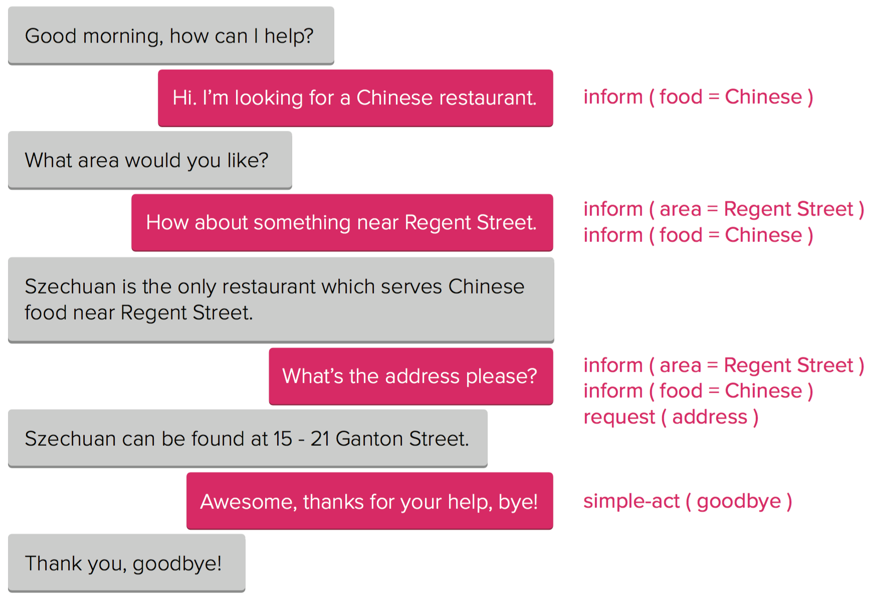
Figure 3: DST labels (user goals given by slot-value pairs) in a multi-turn dialogue Mrkšić et al. (2015).

Post-Specialisation with Other Post-Processors

We also verify that our post-specialisation approach is not tied to the attract-repel method, and is indeed applicable on top of any post-processing specialisation method. We analyse the impact of post-specialisation in the hold-out setting using the original retrofitting (RFit) model Faruqui et al. (2015) and counter-fitting (CFit) Mrkšić et al. (2016) in lieu of attract-repel. The results on word similarity with the best-performing nonlinear-mm variant are summarised in Tab. 2.

The scores again indicate the usefulness of post-specialisation. As expected, the gains are lower than with attract-repel. RFit falls short of CFit as by design it can leverage only synonymy (i.e., attract) external constraints.

	glove		sgns-bow2		fastText
	SL	SV	SL	SV	SL	SV
$\mathbf{X}_{d}$	.408	.286	.414	.275	.383	.255
$\mathbf{X}_{f}$: RFit	.493	.365	.412	.285	.413	.279
$\mathbf{X}_{f}$: CFit	.540	.401	.439	.318	.306	.441

Table 2: Post-specialisation applied to two other post-processing methods. SL: SimLex; SV: SimVerb. Hold-out setting. nonlinear-mm.

5.2 Downstream Task I: DST

Next, we evaluate the usefulness of post-specialisation for two downstream tasks – dialogue state tracking and lexical text simplification – in which discerning semantic similarity from other types of semantic relatedness is crucial. We first evaluate the importance of post-specialisation for a downstream language understanding task of dialogue state tracking (DST) Henderson et al. (2014); Williams et al. (2016), adopting the evaluation protocol and data of Mrkšić et al. (2017).

DST: Model and Evaluation

The DST model is the first component of modern dialogue pipelines Young (2010), which captures the users’ goals at each dialogue turn and then updates the dialogue state. Goals are represented as sets of constraints expressed as slot-value pairs (e.g., food=Chinese). The set of slots and the set of values for each slot constitute the ontology of a dialogue domain. The probability distribution over the possible states is the system’s estimate of the user’s goals, and it is used by the dialogue manager module to select the subsequent system response Su et al. (2016). An example in Fig. 3 illustrates the DST pipeline.

For evaluation, we use the Neural Belief Tracker (NBT), a state-of-the-art DST model which was the first to reason purely over pre-trained word vectors Mrkšić et al. (2017). The NBT uses no hand-crafted semantic lexicons, instead composing word vectors into intermediate utterance and context representations. For full model details, we refer the reader to the original paper. The importance of word vector specialisation for the DST task (e.g., distinguishing between synonyms and antonyms by pulling northern and north closer in the vector space while pushing north and south away) has been established Mrkšić et al. (2017).

English	hold-out	all
Distributional: $\mathbf{X}_{d}$	.797	.797
+ar Spec.: $\mathbf{X}^{\prime}_{s}\cup\mathbf{X}_{u}$	.797	.817
++Mapping: $\mathbf{X}_{f}=\mathbf{X}^{\prime}_{s}\cup\widehat{\mathbf{X}^{\prime}_{u}}$
linear-mm	.815	.818
nonlinear-mm	.827	.835

Table 3: DST results in two evaluation settings (hold-out and all) with different glove variants.

Again, as in prior work the DST evaluation is based on the Wizard-of-Oz (WOZ) v2.0 dataset Wen et al. (2017); Mrkšić et al. (2017), comprising 1,200 dialogues split into training (600 dialogues), development (200), and test data (400). In all experiments, we report the standard DST performance measure: joint goal accuracy, and report scores as averages over 5 NBT training runs.

	German				Italian
	SimLex (Similarity)		WOZ (DST)		SimLex (Similarity)		WOZ (DST)
	hold-out	all	hold-out	all	hold-out	all	hold-out	all
Distributional: $\mathbf{X}_{d}$	.267	.267	.487	.487	.363	.363	.618	.618
+ar Spec.: $\mathbf{X}^{\prime}_{s}\cup\mathbf{X}_{u}$	.267	.422	.487	.535	.363	.616	.618	.634
++Mapping: $\mathbf{X}_{f}$
linear-mm	.354	.449	.485	.533	.401	.616	.627	.633
nonlinear-mm	.367	.466	.496	.538	.428	.616	.637	.647

Table 4: Results on word similarity (Spearman’s $\rho$) and DST (joint goal accuracy) for German and Italian.

Results and Analysis

We again evaluate word vectors in two settings: 1) hold-out, where linguistic constraints with words appearing in the WOZ data are removed, making all WOZ words unseen by attract-repel; and 2) all. The results for the English DST task with different glove word vector variants are summarised in Tab. 3; similar trends in results are observed with two other word vector collections. The scores maintain conclusions established in the word similarity task. First, semantic specialisation with attract-repel is again beneficial, and discerning between synonyms and antonyms improves DST performance. However, specialising unseen words (the final $\mathbf{X}_{u}$ vector space) yields further improvements in both evaluation settings, supporting our claim that the specialisation signal can be propagated to unseen words.

This downstream evaluation again demonstrates the importance of non-linearity, as the peak scores are reported with the nonlinear-mm variant. More substantial gains in the all setup are observed in the DST task compared to the word similarity task. This stems from a lower coverage of the WOZ data in the ar constraints: 36.3% of all WOZ words are unseen words. Finally, the scores are higher on average in the all setup, since this setup uses more external constraints for ar, and consequently uses more training examples to learn the mapping.

Other Languages

We test the portability of our framework to two other languages for which we have similar evaluation data: German (DE) and Italian (IT). SimLex-999 has been translated and rescored in the two languages by Leviant and Reichart (2015), and the WOZ data were translated and adapted by Mrkšić et al. (2017). Exactly the same setup is used as in our English experiments, without any additional language-specific fine-tuning. Linguistic constraints were extracted from the same sources: synonyms from the PPDB (135,868 in DE, 362,452 in IT), antonyms from BabelNet (4,124 in DE, and 16,854 in IT). Our starting distributional vector spaces are taken from prior work: IT vectors are from Dinu et al. (2015), DE vectors are from Vulić and Korhonen (2016a). The results are summarised in Tab. 4.

Our post-specialisation approach yields consistent improvements over the initial distributional space and the ar specialisation model in both tasks and for both languages. We do not observe any gain on IT SimLex in the all setup since IT constraints have almost complete coverage of all IT SimLex words (99.3%; the coverage is 64.8% in German). As expected, the DST scores in the all setup are higher than in the hold-out setup due to a larger number of constraints and training examples.

Lower absolute scores for Italian and German compared to the ones reported for English are due to multiple factors, as discussed previously by Mrkšić et al. (2017): 1) the ar model uses less linguistic constraints for DE and IT; 2) distributional word vectors are induced from smaller corpora; 3) linguistic phenomena (e.g., cases and compounding in DE) contribute to data sparsity and also make the DST task more challenging. However, it is important to stress the consistent gains over the vector space specialised by the state-of-the-art attract-repel model across all three test languages. This indicates that the proposed approach is language-agnostic and portable to multiple languages.

5.3 Downstream Task II: Lexical Simplification

In our second downstream task, we examine the effects of post-specialisation on lexical simplification (LS) in English. LS aims to substitute complex words (i.e., less commonly used words) with their simpler synonyms in the context. Simplified text must keep the meaning of the original text, which is discerning similarity from relatedness is important (e.g., in “The automobile was set on fire” the word “automobile” should be replaced with “car” or “vehicle” but not with “wheel” or “driver”).

Vectors	Specialisation	Acc.	Ch.
	Distributional: $\mathbf{X}_{d}$	66.0	94.0
Glove	+ar Spec.: $\mathbf{X}^{\prime}_{s}\cup\mathbf{X}_{u}$	67.6	87.0
	++Mapping: $\mathbf{X}_{f}$	72.3	87.6
	Distributional: $\mathbf{X}_{d}$	57.8	84.0
fastText	+ar Spec.: $\mathbf{X}^{\prime}_{s}\cup\mathbf{X}_{u}$	69.8	89.4
	++Mapping: $\mathbf{X}_{f}$	74.3	88.8
	Distributional: $\mathbf{X}_{d}$	56.0	79.1
sgns-bow2	+ar Spec.: $\mathbf{X}^{\prime}_{s}\cup\mathbf{X}_{u}$	64.4	86.7
	++Mapping: $\mathbf{X}_{f}$	70.9	86.8

Table 5: Lexical simplification performance with post-specialisation applied on three input spaces.

We employ Light-LS Glavaš and Štajner (2015), a lexical simplification algorithm that: 1) makes substitutions based on word similarities in a semantic vector space, and 2) can be provided an arbitrary embedding space as input. For a complex word, Light-LS considers the most similar words from the vector space as simplification candidates. Candidates are ranked according to several features, indicating simplicity and fitness for the context (semantic relatedness to the context of the complex word). The substitution is made if the best candidate is simpler than the original word. By providing vector spaces post-specialised for semantic similarity to Light-LS, we expect to more often replace complex words with their true synonyms.

We evaluate Light-LS performance in the all setup on the LS benchmark compiled by Horn et al. (2014), who crowdsourced 50 manual simplifications for each complex word. As in prior work, we evaluate performance with the following metrics: 1) Accurracy (Acc.) is the number of correct simplifications made (i.e., the system made the simplification and its substitution is found in the list of crowdsourced substitutions), divided by the total number of indicated complex words; 2) Changed (Ch.) is the percentage of indicated complex words that were replaced by the system (whether or not the replacement was correct).

LS results are summarised in Tab. 5. Post-specialised vector spaces consistently yield 5-6% gain in Accuracy compared to respective distributional vectors and embeddings specialised with the state-of-the-art Attract-Repel model. Similar to DST evaluation, improvements over Attract-Repel demonstrate the importance of specialising the vectors of the entire vocabulary and not only the vectors of words from the external constraints.

6 Conclusion and Future Work

We have presented a novel post-processing model, termed post-specialisation, that specialises word vectors for the full vocabulary of the input vector space. Previous post-processing specialisation models fine-tune word vectors only for words occurring in external lexical resources. In this work, we have demonstrated that the specialisation of the subspace of seen words can be leveraged to learn a mapping function which specialises vectors for all other words, unseen in the external resources. Our results across word similarity and downstream language understanding tasks show consistent improvements over the state-of-the-art specialisation method for all three test languages.

In future work, we plan to extend our approach to specialisation for asymmetric relations such as hypernymy or meronymy Glavaš and Ponzetto (2017); Nickel and Kiela (2017); Vulić and Mrkšić (2018). We will also investigate more sophisticated non-linear functions. The code is available at: https://github.com/cambridgeltl/post-specialisation/.

References

- Al-Rfou et al. (2013) Rami Al-Rfou, Bryan Perozzi, and Steven Skiena. 2013. Polyglot: Distributed word representations for multilingual NLP. In Proceedings of CoNLL, pages 183–192.
- Artetxe et al. (2016) Mikel Artetxe, Gorka Labaka, and Eneko Agirre. 2016. Learning principled bilingual mappings of word embeddings while preserving monolingual invariance. In Proceedings of EMNLP, pages 2289–2294.
- Artetxe et al. (2017) Mikel Artetxe, Gorka Labaka, and Eneko Agirre. 2017. Learning bilingual word embeddings with (almost) no bilingual data. In Proceedings of ACL, pages 451–462.
- Bansal et al. (2014) Mohit Bansal, Kevin Gimpel, and Karen Livescu. 2014. Tailoring continuous word representations for dependency parsing. In Proceedings of ACL, pages 809–815.
- Bian et al. (2014) Jiang Bian, Bin Gao, and Tie-Yan Liu. 2014. Knowledge-powered deep learning for word embedding. In Proceedings of ECML-PKDD, pages 132–148.
- Bojanowski et al. (2017) Piotr Bojanowski, Edouard Grave, Armand Joulin, and Tomas Mikolov. 2017. Enriching word vectors with subword information. Transactions of the ACL, 5:135–146.
- Bruni et al. (2014) Elia Bruni, Nam-Khanh Tran, and Marco Baroni. 2014. Multimodal distributional semantics. Journal of Artificial Intelligence Research, 49:1–47.
- Chen and Manning (2014) Danqi Chen and Christopher D. Manning. 2014. A fast and accurate dependency parser using neural networks. In Proceedings of EMNLP, pages 740–750.
- Collobert et al. (2011) Ronan Collobert, Jason Weston, Léon Bottou, Michael Karlen, Koray Kavukcuoglu, and Pavel P. Kuksa. 2011. Natural language processing (almost) from scratch. Journal of Machine Learning Research, 12:2493–2537.
- Conneau et al. (2017) Alexis Conneau, Guillaume Lample, Marc’Aurelio Ranzato, Ludovic Denoyer, and Hervé Jégou. 2017. Word translation without parallel data. CoRR, abs/1710.04087.
- Cotterell et al. (2016) Ryan Cotterell, Hinrich Schütze, and Jason Eisner. 2016. Morphological smoothing and extrapolation of word embeddings. In Proceedings of ACL, pages 1651–1660.
- Dinu et al. (2015) Georgiana Dinu, Angeliki Lazaridou, and Marco Baroni. 2015. Improving zero-shot learning by mitigating the hubness problem. In Proceedings of ICLR (Workshop Papers).
- Duchi et al. (2011) John C. Duchi, Elad Hazan, and Yoram Singer. 2011. Adaptive subgradient methods for online learning and stochastic optimization. Journal of Machine Learning Research, 12:2121–2159.
- Elfwing et al. (2017) Stefan Elfwing, Eiji Uchibe, and Kenji Doya. 2017. Sigmoid-weighted linear units for neural network function approximation in reinforcement learning. CoRR, abs/1702.03118.
- Faruqui (2016) Manaal Faruqui. 2016. Diverse Context for Learning Word Representations. Ph.D. thesis, Carnegie Mellon University.
- Faruqui et al. (2015) Manaal Faruqui, Jesse Dodge, Sujay Kumar Jauhar, Chris Dyer, Eduard Hovy, and Noah A. Smith. 2015. Retrofitting word vectors to semantic lexicons. In Proceedings of NAACL-HLT, pages 1606–1615.
- Fellbaum (1998) Christiane Fellbaum. 1998. WordNet.
- Finkelstein et al. (2002) Lev Finkelstein, Evgeniy Gabrilovich, Yossi Matias, Ehud Rivlin, Zach Solan, Gadi Wolfman, and Eytan Ruppin. 2002. Placing search in context: The concept revisited. ACM Transactions on Information Systems, 20(1):116–131.
- Frome et al. (2013) Andrea Frome, Gregory S. Corrado, Jonathon Shlens, Samy Bengio, Jeffrey Dean, Marc’Aurelio Ranzato, and Tomas Mikolov. 2013. DeViSE: A deep visual-semantic embedding model. In Proceedings of NIPS, pages 2121–2129.
- Ganitkevitch et al. (2013) Juri Ganitkevitch, Benjamin Van Durme, and Chris Callison-Burch. 2013. PPDB: The Paraphrase Database. In Proceedings of NAACL-HLT, pages 758–764.
- Gerz et al. (2016) Daniela Gerz, Ivan Vulić, Felix Hill, Roi Reichart, and Anna Korhonen. 2016. SimVerb-3500: A large-scale evaluation set of verb similarity. In Proceedings of EMNLP, pages 2173–2182.
- Glavaš and Ponzetto (2017) Goran Glavaš and Simone Paolo Ponzetto. 2017. Dual tensor model for detecting asymmetric lexico-semantic relations. In Proceedings of EMNLP, pages 1758–1768.
- Glavaš and Štajner (2015) Goran Glavaš and Sanja Štajner. 2015. Simplifying lexical simplification: Do we need simplified corpora? In Proceedings of ACL, pages 63–68.
- Glorot and Bengio (2010) Xavier Glorot and Yoshua Bengio. 2010. Understanding the difficulty of training deep feedforward neural networks. In Proceedings of AISTATS, pages 249–256.
- Harris (1954) Zellig S. Harris. 1954. Distributional structure. Word, 10(23):146–162.
- He et al. (2015) Kaiming He, Xiangyu Zhang, Shaoqing Ren, and Jian Sun. 2015. Delving deep into rectifiers: Surpassing human-level performance on ImageNet classification. In Proceedings of ICCV, pages 1026–1034.
- Henderson et al. (2014) Matthew Henderson, Blaise Thomson, and Jason D. Wiliams. 2014. The Second Dialog State Tracking Challenge. In Proceedings of SIGDIAL, pages 263–272.
- Hill et al. (2015) Felix Hill, Roi Reichart, and Anna Korhonen. 2015. SimLex-999: Evaluating semantic models with (genuine) similarity estimation. Computational Linguistics, 41(4):665–695.
- Hochreiter and Schmidhuber (1997) Sepp Hochreiter and Jürgen Schmidhuber. 1997. Long Short-Term Memory. Neural Computation, 9(8):1735–1780.
- Horn et al. (2014) Colby Horn, Cathryn Manduca, and David Kauchak. 2014. Learning a lexical simplifier using wikipedia. In Proceedings of the ACL, pages 458–463.
- Kiela et al. (2015) Douwe Kiela, Felix Hill, and Stephen Clark. 2015. Specializing word embeddings for similarity or relatedness. In Proceedings of EMNLP, pages 2044–2048.
- Kim et al. (2016) Joo-Kyung Kim, Gokhan Tur, Asli Celikyilmaz, Bin Cao, and Ye-Yi Wang. 2016. Intent detection using semantically enriched word embeddings. In Proceedings of SLT.
- Kingma and Ba (2015) Diederik P. Kingma and Jimmy Ba. 2015. Adam: A method for stochastic optimization. In Proceedings of ICLR (Conference Track).
- Kipfer (2009) Barbara Ann Kipfer. 2009. Roget’s 21st Century Thesaurus (3rd Edition). Philip Lief Group.
- Klambauer et al. (2017) Günter Klambauer, Thomas Unterthiner, Andreas Mayr, and Sepp Hochreiter. 2017. Self-normalizing neural networks. CoRR, abs/1706.02515.
- Kummerfeld et al. (2015) Jonathan K. Kummerfeld, Taylor Berg-Kirkpatrick, and Dan Klein. 2015. An empirical analysis of optimization for max-margin NLP. In Proceedings of EMNLP, pages 273–279.
- Lazaridou et al. (2015) Angeliki Lazaridou, Georgiana Dinu, and Marco Baroni. 2015. Hubness and pollution: Delving into cross-space mapping for zero-shot learning. In Proceedings of ACL, pages 270–280.
- Leviant and Reichart (2015) Ira Leviant and Roi Reichart. 2015. Separated by an un-common language: Towards judgment language informed vector space modeling. CoRR, abs/1508.00106.
- Levy and Goldberg (2014) Omer Levy and Yoav Goldberg. 2014. Dependency-based word embeddings. In Proceedings of ACL, pages 302–308.
- Levy et al. (2015) Omer Levy, Yoav Goldberg, and Ido Dagan. 2015. Improving distributional similarity with lessons learned from word embeddings. Transactions of the ACL, 3:211–225.
- Li et al. (2016) Sihan Li, Jiantao Jiao, Yanjun Han, and Tsachy Weissman. 2016. Demystifying ResNet. CoRR, abs/1611.01186.
- Liu et al. (2015) Quan Liu, Hui Jiang, Si Wei, Zhen-Hua Ling, and Yu Hu. 2015. Learning semantic word embeddings based on ordinal knowledge constraints. In Proceedings of ACL, pages 1501–1511.
- Maas et al. (2013) Andrew L. Maas, Awni Y. Hannun, and Andrew Y. Ng. 2013. Rectifier nonlinearities improve neural network acoustic models. In Proceedings of ICML.
- Melamud et al. (2016a) Oren Melamud, Jacob Goldberger, and Ido Dagan. 2016a. Context2vec: Learning generic context embedding with bidirectional LSTM. In Proceedings of CoNLL, pages 51–61.
- Melamud et al. (2016b) Oren Melamud, David McClosky, Siddharth Patwardhan, and Mohit Bansal. 2016b. The role of context types and dimensionality in learning word embeddings. In Proceedings of NAACL-HLT, pages 1030–1040.
- Mikolov et al. (2013a) Tomas Mikolov, Quoc V. Le, and Ilya Sutskever. 2013a. Exploiting similarities among languages for machine translation. arXiv preprint, CoRR, abs/1309.4168.
- Mikolov et al. (2013b) Tomas Mikolov, Ilya Sutskever, Kai Chen, Gregory S. Corrado, and Jeffrey Dean. 2013b. Distributed representations of words and phrases and their compositionality. In Proceedings of NIPS, pages 3111–3119.
- Mishkin and Matas (2016) Dmytro Mishkin and Jiri Matas. 2016. All you need is a good init. In Proceedings of ICLR (Conference Track).
- Mrkšić et al. (2017) Nikola Mrkšić, Diarmuid Ó Séaghdha, Tsung-Hsien Wen, Blaise Thomson, and Steve Young. 2017. Neural belief tracker: Data-driven dialogue state tracking. In Proceedings of ACL, pages 1777–1788.
- Mrkšić et al. (2015) Nikola Mrkšić, Diarmuid Ó Séaghdha, Blaise Thomson, Milica Gašić, Pei-Hao Su, David Vandyke, Tsung-Hsien Wen, and Steve Young. 2015. Multi-domain dialog state tracking using recurrent neural networks. In Proceedings of ACL, pages 794–799.
- Mrkšić et al. (2016) Nikola Mrkšić, Diarmuid Ó Séaghdha, Blaise Thomson, Milica Gašić, Lina Maria Rojas-Barahona, Pei-Hao Su, David Vandyke, Tsung-Hsien Wen, and Steve Young. 2016. Counter-fitting word vectors to linguistic constraints. In Proceedings of NAACL-HLT.
- Mrkšić et al. (2017) Nikola Mrkšić, Ivan Vulić, Diarmuid Ó Séaghdha, Ira Leviant, Roi Reichart, Milica Gašić, Anna Korhonen, and Steve Young. 2017. Semantic specialisation of distributional word vector spaces using monolingual and cross-lingual constraints. Transactions of the ACL, 5:309–324.
- Nair and Hinton (2010) Vinod Nair and Geoffrey E. Hinton. 2010. Rectified linear units improve restricted Boltzmann machines. In Proceedings of ICML, pages 807–814.
- Navigli and Ponzetto (2012) Roberto Navigli and Simone Paolo Ponzetto. 2012. BabelNet: The automatic construction, evaluation and application of a wide-coverage multilingual semantic network. Artificial Intelligence, 193:217–250.
- Nguyen et al. (2017) Kim Anh Nguyen, Maximilian Köper, Sabine Schulte im Walde, and Ngoc Thang Vu. 2017. Hierarchical embeddings for hypernymy detection and directionality. In Proceedings of EMNLP, pages 233–243.
- Nguyen et al. (2016) Kim Anh Nguyen, Sabine Schulte im Walde, and Ngoc Thang Vu. 2016. Integrating distributional lexical contrast into word embeddings for antonym-synonym distinction. In Proceedings of ACL, pages 454–459.
- Nickel and Kiela (2017) Maximilian Nickel and Douwe Kiela. 2017. Poincaré embeddings for learning hierarchical representations. In Proceedings of NIPS.
- Ono et al. (2015) Masataka Ono, Makoto Miwa, and Yutaka Sasaki. 2015. Word embedding-based antonym detection using thesauri and distributional information. In Proceedings of NAACL-HLT, pages 984–989.
- Osborne et al. (2016) Dominique Osborne, Shashi Narayan, and Shay Cohen. 2016. Encoding prior knowledge with eigenword embeddings. Transactions of the ACL, 4:417–430.
- Pavlick et al. (2015) Ellie Pavlick, Pushpendre Rastogi, Juri Ganitkevitch, Benjamin Van Durme, and Chris Callison-Burch. 2015. PPDB 2.0: Better paraphrase ranking, fine-grained entailment relations, word embeddings, and style classification. In Proceedings of ACL, pages 425–430.
- Pennington et al. (2014) Jeffrey Pennington, Richard Socher, and Christopher Manning. 2014. Glove: Global vectors for word representation. In Proceedings of EMNLP, pages 1532–1543.
- Ramachandran et al. (2017) Prajit Ramachandran, Barret Zoph, and Quoc V. Le. 2017. Searching for activation functions. CoRR, abs/1710.05941.
- Rothe and Schütze (2015) Sascha Rothe and Hinrich Schütze. 2015. AutoExtend: Extending word embeddings to embeddings for synsets and lexemes. In Proceedings of ACL, pages 1793–1803.
- Ruder et al. (2017) Sebastian Ruder, Ivan Vulić, and Anders Søgaard. 2017. A survey of cross-lingual embedding models. CoRR, abs/1706.04902.
- Schwartz et al. (2015) Roy Schwartz, Roi Reichart, and Ari Rappoport. 2015. Symmetric pattern based word embeddings for improved word similarity prediction. In Proceedings of CoNLL, pages 258–267.
- Su et al. (2016) Pei-Hao Su, Milica Gašić, Nikola Mrkšić, Lina Rojas-Barahona, Stefan Ultes, David Vandyke, Tsung-Hsien Wen, and Steve Young. 2016. Continuously learning neural dialogue management. In arXiv preprint: 1606.02689.
- Vulić and Korhonen (2016a) Ivan Vulić and Anna Korhonen. 2016a. Is "universal syntax" universally useful for learning distributed word representations? In Proceedings of ACL, pages 518–524.
- Vulić and Korhonen (2016b) Ivan Vulić and Anna Korhonen. 2016b. On the role of seed lexicons in learning bilingual word embeddings. In Proceedings of ACL, pages 247–257.
- Vulić and Mrkšić (2018) Ivan Vulić and Nikola Mrkšić. 2018. Specialising word vectors for lexical entailment. In Proceedings of NAACL-HLT.
- Vulić et al. (2017a) Ivan Vulić, Nikola Mrkšić, and Anna Korhonen. 2017a. Cross-lingual induction and transfer of verb classes based on word vector space specialisation. In Proceedings of EMNLP, pages 2536–2548.
- Vulić et al. (2017b) Ivan Vulić, Nikola Mrkšić, Roi Reichart, Diarmuid Ó Séaghdha, Steve Young, and Anna Korhonen. 2017b. Morph-fitting: Fine-tuning word vector spaces with simple language-specific rules. In Proceedings of ACL, pages 56–68.
- Wen et al. (2017) Tsung-Hsien Wen, David Vandyke, Nikola Mrkšić, Milica Gašić, Lina M. Rojas-Barahona, Pei-Hao Su, Stefan Ultes, and Steve Young. 2017. A network-based end-to-end trainable task-oriented dialogue system. In Proceedings of EACL.
- Weston et al. (2011) Jason Weston, Samy Bengio, and Nicolas Usunier. 2011. WSABIE: Scaling up to large vocabulary image annotation. In Proceedings of IJCAI, pages 2764–2770.
- Wieting et al. (2015) John Wieting, Mohit Bansal, Kevin Gimpel, and Karen Livescu. 2015. From paraphrase database to compositional paraphrase model and back. Transactions of the ACL, 3:345–358.
- Williams et al. (2016) Jason D. Williams, Antoine Raux, and Matthew Henderson. 2016. The Dialog State Tracking Challenge series: A review. Dialogue & Discourse, 7(3):4–33.
- Xu et al. (2014) Chang Xu, Yalong Bai, Jiang Bian, Bin Gao, Gang Wang, Xiaoguang Liu, and Tie-Yan Liu. 2014. RC-NET: A general framework for incorporating knowledge into word representations. In Proceedings of CIKM, pages 1219–1228.
- Young (2010) Steve Young. 2010. Cognitive User Interfaces. IEEE Signal Processing Magazine.
- Yu and Dredze (2014) Mo Yu and Mark Dredze. 2014. Improving lexical embeddings with semantic knowledge. In Proceedings of ACL, pages 545–550.
- Zhang et al. (2014) Jingwei Zhang, Jeremy Salwen, Michael Glass, and Alfio Gliozzo. 2014. Word semantic representations using bayesian probabilistic tensor factorization. In Proceedings of EMNLP, pages 1522–1531.