Global well-posedness and scattering for the defocusing $\dot{H}^{\frac{1}{2}}$-critical nonlinear Schrödinger equation in $\mathbb{R}^{2}$

Abstract.

In this paper we consider the Cauchy initial value problem for the defocusing quintic nonlinear Schrödinger equation in two dimensions with general data in the critical space $\dot{H}^{\frac{1}{2}}(\mathbb{R}^{2})$. We show that if a solution remains bounded in $\dot{H}^{\frac{1}{2}}(\mathbb{R}^{2})$ in its maximal interval of existence, then the interval is infinite and the solution scatters.

1. Introduction

In the past two decades, there has been significant progress in the understanding of the long time dynamics (existence, uniqueness and scattering) in various regimes of the defocusing nonlinear Schrödinger equation (NLS) on $\mathbb{R}^{d}$

$$\begin{cases}i\partial_{t}u+\Delta u=\operatorname{}\left|u\right|^{p-1}u,\\ u(0,x)=u_{0}(x),\end{cases}$$ (1.1)

where $u:\mathbb{R}_{t}\times\mathbb{R}_{x}^{d}\to\mathbb{C}$ is a complex-valued function of time and space and $p>1$.

The equation (1.1) enjoys several symmetries and invariances among which the most important one is the scaling symmetry. That is, if $u$ solves (1.1) with initial data $u_{0}$, then $u_{\lambda}(t,x)=\lambda^{\frac{2}{p-1}}u(\lambda^{2}t,\lambda x)$ solves (1.1) with initial data $u_{0,\lambda}(x)=\lambda^{\frac{2}{p-1}}u_{0}(\lambda x)$ and $\operatorname{}\left\|u_{0,\lambda}\right\|_{\dot{H}^{s}}=\operatorname{}\left\|u_{0}\right\|_{\dot{H}^{s}}$, for any $\lambda\in\mathbb{R}$. The problem becomes scale invariant when the data belongs to the homogenous Sobolev space $\dot{H}^{\frac{d}{2}-\frac{2}{p-1}}(\mathbb{R}^{d})$. We refer to this regularity index as critical relative to scaling and denote it by $s_{c}:=\frac{d}{2}-\frac{2}{p-1}$.

For data in $H^{s}(\mathbb{R}^{d})$ with $s>s_{c}$ (sub-critical regime) local well-posedness (local in time existence, uniqueness and continuous dependence of the data to solution map) follows from the Strichartz estimates and a fixed point argument with a time of existence depending solely on the $H^{s}$ norm of the data. A similar argument gives also local well-posedness for data in $\dot{H}^{s_{c}}(\mathbb{R}^{d})$ but in this case the time of existence depends also on the profile of the data [7, 8, 9, 6].

The equation (1.1) conserves the mass,

$$M(u(t)):=\int_{\mathbb{R}^{d}}\operatorname{}\left|u(t,x)\right|^{2}\,dx=M(u_{0}),$$ (1.2)

and the energy,

$$E(u(t)):=\int_{\mathbb{R}^{d}}\frac{1}{2}\operatorname{}\left|\nabla u(t,x)\right|^{2}+\frac{1}{p+1}\operatorname{}\left|u(t,x)\right|^{p+1}\,dx=E(u_{0}).$$ (1.3)

The equation (1.1) also conserves momentum,

$$\mathcal{P}(u(t)):=\int_{\mathbb{R}^{d}}\operatorname{Im}[\bar{u}(t,x)\nabla u(t,x)]\,dx=\mathcal{P}(u_{0}),$$ (1.4)

which plays a fundamental role in the derivation of the interaction Morawetz estimates [13, 50, 11, 12]. It should be noted however that it does not control the $\dot{H}^{\frac{1}{2}}$ norm globally in time.

In the energy-subcritical regime ($s_{c}<1$), the conservation of energy gives global well-posedness in $H^{1}$ by iteration, but this does not give scattering (see Definition 1.3 for details). In the energy-critical regime (see [9, 6]), as we mentioned, the time of existence depends on the profile of the data as well. In this case, if the energy of the initial data is given to be small enough, hence the profile also sufficiently small, then the solution is known to exist globally in time, and scatters.

In the energy-critical regime ($s_{c}=1$, $p=1+\frac{4}{d-2}$) with large initial data, one cannot, however, iterate the time of existence to obtain a global solution, because the time of existence depends also on the profile of the data (not a conserved quantity), which may lead to a shrinking interval of existence when iterating the local well-posedness theorem.

Similarly, in the mass-subcritical regime ($s_{c}<s=0$), the conservation of mass gives global well-posedness in $L^{2}$ (eg. cubic NLS on $\mathbb{R}$, $s_{c}=-\frac{1}{2}$) while if $s_{c}=0$, $p=1+\frac{4}{d}$, one cannot extend the local given solution to a global solution by iteration due to the same reason.

The two special cases when the equation becomes scale invariant at the level of one of the conserved quantities (1.2) and (1.3) have received special attention in the past. These are called the mass-critical NLS ($s_{c}=0$,  $p=1+\frac{4}{d}$) and the energy-critical NLS ($s_{c}=1$,   $p=1+\frac{4}{d-2}$). In these two regimes, it is sufficient to prove a uniform a priori bound for the spacetime $L_{t,x}^{\frac{2(d+2)}{d-2s_{c}}}$ norm of solutions to the critical NLS, since it is now standard (see [8, 9, 6]) to show that such a bound gives global well-posedness and scattering for general data.

In the energy-critical case, Bourgain [2] first introduced an inductive argument on the size of the energy and a refined Morawetz inequality to prove global existence and scattering in three dimensions for large finite energy data which is assumed to be radial. A different proof of the same result is given in [23]. A key ingredient in the latter proof is an a priori estimate of the time average of local energy over a parabolic cylinder, which plays a similar role as Bourgain’s refined Morawetz inequality. Then, a breakthrough was made by Colliander-Keel-Staffilani-Takaoka-Tao [14]. They removed the radial assumption and proved global well-posedness and scattering of the energy-critical problem in three dimensions for general large data. They relied on Bourgain’s induction on energy technique to find minimal blow-up solutions that concentrate in both physical and frequency spaces, and proved new interaction Morawetz-type estimates to rule out this kind of minimal blow-up solutions. Later [51, 60] extended the result in [14] to higher dimensions.

In [28] Kenig and Merle proposed a new methodology, a deep and broad road map to tackle critical problems. In fact, using a contradiction argument they first proved the existence of a critical element such that the global well-posedness and scattering fail. Then relying on a concentration compactness argument they showed that this critical element enjoys a compactness property up to the symmetries of this equation. This final step was reduced to a rigidity theorem that precluded the existence of such critical element. In this form they were able to prove in particular the global well-posedness and scattering for the focusing radially symmetric energy critical Schrödinger equation in dimensions three four and five under suitable conditions on the data (Namely, that the energy and the $\dot{H}^{1}$ norm of the data are less than those of the ground state). Following their road map Kenig and Merle also showed [29] the global well-posedness and scattering for the focusing energy-critical wave equation. It is worth mentioning that the concentration compactness method that they applied was first introduced in the context of Sobolev embeddings in [19], nonlinear wave equations in [1] and Schrödinger equations in [44, 31, 32].

The mass-critical global well-posedness and scattering problem was also first studied in the radial case as in [57, 36]. Then Dodson proved the global well-posedness of the mass-critical problem in any dimension for nonradial data [15, 16, 17]. A key ingredient in Dodson’s work is to prove a long time Strichartz estimate to rule out minimal blow-up solutions. Such estimate also helps to derive a frequency localized Morawetz-type estimate. Furthermore, in dimension one [16] and in dimensions two [17], Dodson introduced suitable versions of atomic spaces to deal with the failure of the endpoint Strichartz estimates in these cases. It should be noted that the interaction Morawetz estimates proved in [50] played a fundamental role in ruling out one type of minimal blow-up solutions. Moreover the bilinear estimates in [17] that gave a logarithmic improvement over Bourgain’s bilinear estimteas also relied on the interaction Morawetz estimates of [50]. For dispersive equations, low dimension settings are less favorable due to the weaker time decay. This paper in fact deals with this type of setup.

Unlike the energy- and mass-critical problems, for any other $s_{c}\neq 0,1$, there are no conserved quantities that control the growth in time of the $\dot{H}^{s_{c}}$ norm of the solutions. In [30], Kenig and Merle showed for the first time that if a solution of the defocusing cubic NLS in three dimensions remains bounded in the critical norm $\dot{H}^{\frac{1}{2}}$ in the maximal time of existence, then the interval of existence is infinite and the solution scatters using concentration compactness and rigidity argument. [48] extended the $\dot{H}^{\frac{1}{2}}$ critical result in [30] to dimensions four and higher (some other inter-critical problems were also treated in [47, 49]). However, the analogue of the $\dot{H}^{\frac{1}{2}}$-critical result in dimensions two remained open. This was because:

1. the interaction Morawetz estimates in two dimensions are significantly different from those in dimensions three and above,

2. and the endpoint Strichartz estimate fails.

In this paper, we focus on how to close this gap. More precisely, we consider the Cauchy problem for the defocusing $\dot{H}^{\frac{1}{2}}$-critical quintic Schrödinger equation in $\mathbb{R}^{1+2}$:

$$\begin{cases}i\partial_{t}u+\Delta u=\operatorname{}\left|u\right|^{4}u,\\ u(0,x)=u_{0}(x)\in\dot{H}^{\frac{1}{2}}(\mathbb{R}^{2}),\end{cases}$$ (1.5)

with $u:\mathbb{R}_{t}\times\mathbb{R}_{x}^{2}\to\mathbb{C}$.

The main result is:

Theorem 1.1 (Main theorem).

Let $u:I\times\mathbb{R}^{2}\to\mathbb{C}$ be a maximal-lifespan solution to (1.5) such that $u\in L_{t}^{\infty}\dot{H}_{x}^{\frac{1}{2}}(I\times\mathbb{R}^{2})$. Then $u$ is global and scatters (see Definition 1.3), with

$$\int_{\mathbb{R}}\int_{\mathbb{R}^{2}}\operatorname{}\left|u(t,x)\right|^{8}\,dxdt\leq C\operatorname{}\left(\operatorname{}\left\|u\right\|_{L_{t}^{\infty}\dot{H}_{x}^{\frac{1}{2}}(\mathbb{R}\times\mathbb{R}^{2})}\right)$$ (1.6)

for some function $C:[0,\infty)\to[0,\infty)$.

In order to prove a uniform a priori bound for the spacetime $L_{t,x}^{8}$ norm of solutions, following the road map by Kenig and Merle, one proceeds by contradiction as follows:

1. First assume that the spacetime norm in (1.6) is unbounded for large data. Then the fact that for sufficiently small initial data the solutions are globally well-posed and their spacetime norms are bounded, imply the existence of a special class of solutions (called minimal blow-up solutions, see Definition 1.7) that are concentrated in both space and frequency.

2. One then precludes the existence of minimal blow-up solutions by conservation laws and suitable (frequency localized interaction) Morawetz estimates.

It is shown in [30, 48] that a minimal blow-up solution $u:I\times\mathbb{R}^{d}\to\mathbb{C}$ ($d\geq 3$) must concentrate around some spatial center $x(t)$ and at some frequency scale $N(t)$ at any time $t$ in the interval of existence (Step 1). We can extend this to $\mathbb{R}^{2}$. Then in the step to rule out the possibility of minimal blow-up solutions (Step 2), we employ the effective tools given by Morawetz estimates. For dimensions three and higher, the Morawetz estimates introduced in [43] are given by:

$$\int_{I}\int_{\mathbb{R}^{d}}\frac{\operatorname{}\left|u(t,x)\right|^{p+1}}{\operatorname{}\left|x\right|}\,dxdt\lesssim\operatorname{}\left\|u\right\|_{L_{t}^{\infty}\dot{H}_{x}^{\frac{1}{2}}(I\times\mathbb{R}^{d})}^{2}.$$ (1.7)

Note that the upper bound on the right-hand side depends only on the $\dot{H}^{\frac{1}{2}}$ norm of the solutions, so it is relatively easy to handle in the $\dot{H}^{\frac{1}{2}}$-critical regime. These were the Morawetz estimates used in [30, 48]. However in dimensions two, (1.7) does not hold. We employ instead the interaction Morawetz estimates, which were first introduced in [13] in dimensions three and then extended to dimensions four and higher in [51]:

$$-\int_{I}\iint_{\mathbb{R}^{d}\times\mathbb{R}^{d}}\operatorname{}\left|u(t,x)\right|^{2}\Delta\operatorname{}\left(\frac{1}{\operatorname{}\left|x-y\right|}\right)\operatorname{}\left|u(t,y)\right|^{2}\,dxdydt$$

$$\lesssim\operatorname{}\left\|u\right\|_{L_{t}^{\infty}L_{x}^{2}(I\times\mathbb{R}^{d})}^{2}\operatorname{}\left\|u\right\|_{L_{t}^{\infty}\dot{H}_{x}^{\frac{1}{2}}(I\times\mathbb{R}^{d})}^{2}.$$

In dimensions two, the following interaction Morawetz estimate was proved as in [50, 11, 12]:

$$\operatorname{}\left\|\operatorname{}\left|\nabla\right|^{\frac{1}{2}}\operatorname{}\left|u(t,x)\right|^{2}\right\|_{L_{t,x}^{2}(I\times\mathbb{R}^{2})}^{2}\lesssim\operatorname{}\left\|u\right\|_{L_{t}^{\infty}L_{x}^{2}(I\times\mathbb{R}^{2})}^{2}\operatorname{}\left\|u\right\|_{L_{t}^{\infty}\dot{H}_{x}^{\frac{1}{2}}(I\times\mathbb{R}^{2})}^{2}.$$ (1.8)

Note that the upper bound above depends on the $\dot{H}^{\frac{1}{2}}$ norm as well as on the $L^{2}$ norm of the solutions. Hence in our case the right hand side does not need to be finite since there is no a priori bound on $\operatorname{}\left\|u(t)\right\|_{L_{x}^{2}}$. In contrast, the upper bounds of the Morawetz estimates (1.7) used in [30, 48] depend only on $\dot{H}^{\frac{1}{2}}$ norm. If we were able to prove an analogue of (1.7) in two dimensions (which never holds), we would obtain a bounded spacetime norm immediately and complete Step 2 in the road map by simply adapting the argument in [30] to two dimensions. So the difference in the Morawetz estimates raises a headache issue. However, if we truncate the solutions to high frequencies, the right-hand side of (1.8) will be finite. As a result, we need to have a good estimate for the error produced in this procedure. Moreover, (1.8) scales like $\int_{I}N(t)\,dt$ (here recall $N(t)$ is the concentration radius of minimal blow-up solutions in the frequency space). Intuitively, the interaction Morawetz estimates are expected to help us to rule out the existence for the solutions satisfying $\int_{0}^{T_{max}}N(t)\,dt=\infty$.

More precisely, we use the criteria whether $T_{max}(:=\sup I)$ and $\int_{0}^{T_{max}}N(t)\,dt$ are finite or infinite to classify minimal blow-up solutions ($I$ is the maximal time interval, see Definition 1.2):

	$T_{max}<\infty$	$T_{max}=\infty$
$\int_{0}^{T_{max}}N(t)\,dt<\infty$	I	II
$\int_{0}^{T_{max}}N(t)\,dt=\infty$	III	IV

where

• I, III are called finite-time blow-up solutions

• I, II are called frequency cascade solutions

• III, IV are called quasi-soliton solutions.

In $\dot{H}^{\frac{1}{2}}$ critical regime, it happens that $\int_{0}^{T_{max}}N(t)\,dt<\infty$ implies $T_{max}<\infty$, hence all frequency cascade solutions are also finite-time blow-up solutions, i.e. there is no Case II in this setting. Now we proceed to rule out the existence of minimal blow-up solutions case by case.

Cases III, IV (quasi-soliton solutions)

These are the cases that we expect the interaction Morawetz estimates will help us to rule out. To deal with these cases, we truncate the solutions to high frequencies, just as it was done in [14, 51, 60] for the energy-critical problem in dimensions three and above. As a result, we need to derive the more involved good estimate for the low frequency component of the solutions. Here, we recall some ideas and strategies from [15, 16, 17].

In the mass-critical problem, Dodson [15, 16, 17] truncated the solutions to low frequency, since the low frequency component of the solutions was bounded under the $\dot{H}^{\frac{1}{2}}$ norm. (The cutoff in the mass-critical problem and the cutoff in the $\dot{H}^{\frac{1}{2}}$-critical regime are opposite.) To estimate the errors produced by truncating to low frequency, a suitable bound over the high frequency is needed, hence Dodson [15] introduced the long time Strichartz estimates in dimensions three and higher:

$$\operatorname{}\left\|P_{\operatorname{}\left|\xi-\xi(t)\right|>N}u\right\|_{L_{t}^{2}L_{x}^{\frac{2d}{d-2}}(J\times\mathbb{R}^{d})}\lesssim\operatorname{}\left(\frac{K}{N}\right)^{\frac{1}{2}}+1,$$ (1.9)

where $J$ is an interval satisfying

$$\int_{J}N(t)^{3}\,dt=K.$$

Note that $\int_{J}N(t)^{3}\,dt$ scales like (1.8) in the mass-critical regime, and it plays the same role as $\int_{J}N(t)\,dt$ in our setting.

To obtain (1.9) one requires the endpoint Strichartz estimate $L_{t}^{2}L_{x}^{\frac{2d}{d-2}}$. For $d\geq 3$ the endpoint estimate holds, see [27], however in dimensions two, as in [54, 56], it was shown that the $L_{t}^{2}L_{x}^{\infty}$ endpoint fails. This failure causes the great difficulty for defining and proving the long time Strichartz estimates. To conquer this defect, Dodson [17] constructed a new function space out of a certain atomic spaces in dimensions two. This construction captured the essential features of the long time Strichartz estimates (1.9) in dimensions three and higher.

Back to our case, we follow Dodson’s idea in [17] and construct a similar but ‘upside-down’ version of a long time Strichartz estimate adapted to the $\dot{H}^{\frac{1}{2}}$-critical setting. Our ‘upside-down’ method is because in the mass-critical regime, Dodson [17] lost the a priori control in the $\dot{H}^{\frac{1}{2}}$-norm and used the long time Strichartz to quantify how bad $\dot{H}^{\frac{1}{2}}$-norm is out of control, while we lose the a priori control of $L^{2}$-norm. Hence we define a long time Strichartz estimate over low frequency and expect that it gives a good control of the low frequency components of the solutions. Moreover, in our proof of the long time Strichartz estimate, we should be very careful with the high frequency and high frequency interaction into low frequency terms in Littlewood-Paley decomposition. It is because such terms require more summability due to the construction of the atomic spaces where the long time Strichartz estimate lives. This forces us to gain more decay than the mass-critical case to sum over the high frequency terms. In contrast, these terms were not problematic in mass-critical [17], because with the opposite cutoff the worse case was all low frequencies interaction into high frequency. However, this case never happens since the contribution of all low frequencies remains low. With the error terms settled, the frequency localized Morawetz estimate will help us to preclude the existence of the quasi-soliton solutions.

Case I (finite-time blow-up solutions)

Next, we are left to rule out Case I. In $\dot{H}^{s_{c}}$ regime ($s_{c}\neq\frac{1}{2}$), see [35, 15, 16, 17, 47], long time Strichartz estimates help to prove either additional decay or additional regularity for the solutions belonging to Cases I, II, as a result, the solutions in these cases can be shown to have zero mass or energy, which contradicts the fact they are blow-up solutions. However, in the $\dot{H}^{\frac{1}{2}}$ critical regime, due to the scaling, the long time Strichartz estimates do not provide any additional decay as we would like. This forces us to treat Case I as finite-time blow-up solutions, instead of as frequency cascade solutions. Since we do not need the additional information from $\int N(t)\,dt$, we are allowed to consider the finite-time blow-up solutions (Cases I, III) together. In these cases, by considering the rate of change (in time) of the mass of solutions restricted within a spacial bump and using the finiteness of blow-up time, we can see the impossibility of this type of minimal blow-up solutions.

1.1. A more formal outline of the proof

We first define

Definition 1.2 (Solution).

A function $u:I\times\mathbb{R}^{2}\to C$ on a time interval $I(\ni 0)$ is a solution to (1.5) if it belongs to $C_{t}\dot{H}_{x}^{\frac{1}{2}}(K\times\mathbb{R}^{2})\cap L_{t,x}^{8}(K\times\mathbb{R}^{2})$ for every compact $K\subset I$ and obeys the Duhamel formula

$$u(t)=e^{it\Delta}u_{0}-i\int_{0}^{t}e^{i(t-t^{\prime})\Delta}\operatorname{}\left(\operatorname{}\left|u\right|^{4}u\right)(t^{\prime},x)\,dt^{\prime}$$

for all $t\in I$. We call $I$ the lifespan of $u$; we say $u$ is a maximal-lifespan solution if it cannot be extended to any strictly larger interval. If $I=R$, we say $u$ is global.

Definition 1.3 (Scattering).

A solution to (1.5) is said to scatter forward (or backward) in time if there exist $u_{\pm}\in\dot{H}^{\frac{1}{2}}(\mathbb{R}^{2})$ such that

$$\lim\limits_{t\to\pm\infty}\operatorname{}\left\|u(t)-e^{it\Delta}u_{\pm}\right\|_{\dot{H}_{x}^{\frac{1}{2}}(\mathbb{R}^{2})}=0.$$

Definition 1.4 (Scattering size and blow up).

We define the scattering size of a solution $u$ to (1.5) on a time interval $I$ by

$$S_{I}(u)=\int_{I}\int_{\mathbb{R}^{2}}\operatorname{}\left|u(t,x)\right|^{8}\,dxdt.$$

If there exists $t\in I$ such that $S_{[t,\sup I)}(u)=\infty$, then we say $u$ blows up forward in time. Similarly, if there exists $t\in I$ such that $S_{(\inf I,t]}(u)=\infty$, then we say $u$ blows up backward in time.

The local theory for (1.5) has been worked out by Cazenave-Weissler [7, 8, 9, 6].

Theorem 1.5 (Local well-posedness).

Assume $u_{0}\in\dot{H}^{\frac{1}{2}}(\mathbb{R}^{2})$. Then there exists a unique maximal-lifespan solution $u:I\times\mathbb{R}^{2}\to\mathbb{C}$ to (1.5) such that:

1. (Local existence) $I$ is an open interval containing $0$.

2. (Blowup criterion) If $\sup I$ is finite, then the solution $u$ blows up forward in time. If $\inf I$ is finite, then the solution $u$ blows up backward in time.

3. (Scattering) If $u$ does not blow up forward in time then $\sup I=\infty$ and u scatters forward in time. If $u$ does not blow up backward in time then $\inf I=\infty$ and u scatters backward in time.

4. (Small-data global existence) If $\operatorname{}\left\|u_{0}\right\|_{\dot{H}_{x}^{\frac{1}{2}}}$ is sufficiently small then the solution $u$ is global, scatters and does not blow up either forward or backward in time, with $S_{\mathbb{R}}(u)\lesssim\operatorname{}\left\|u_{0}\right\|_{\dot{H}_{x}^{\frac{1}{2}}}^{8}$

To prove Theorem 1.1, we, following the road map in [28], argue by contradiction. First, define $L:[0,\infty)\to[0,\infty]$ by

$$L(E):=\sup\operatorname{}\left\{S_{I}(u)\big{|}u:I\times\mathbb{R}^{2}\to\mathbb{C}\text{ solving }\eqref{NLS}\text{ with }\operatorname{}\left\|u\right\|_{L_{t}^{\infty}\dot{H}_{x}^{\frac{1}{2}}(I\times\mathbb{R}^{2})}^{2}\leq E\right\}.$$

Note that $L(E)$ is a non-negative, non-decreasing and continuous function satisfying $L(E)\leq E^{4}$ for $E$ sufficiently small. Then there must exist a unique critical threshold $E_{c}\in(0,\infty]$ such that

$$L(E)\begin{cases}<\infty\quad\text{ if }E<E_{c}\\ =\infty\quad\text{ if }E\geq E_{c}.\end{cases}$$

The failure of main theorem implies that $0<E_{c}<\infty$. Moreover,

Theorem 1.6 (Existence of minimal counterexamples).

Suppose Theorem 1.1 fails to be true. Then there exists a critical energy $0<E_{c}<\infty$ and a maximal-lifespan solution $u:I\times\mathbb{R}^{2}\to\mathbb{C}$ to (1.5) with $\operatorname{}\left\|u\right\|_{L_{t}^{\infty}\dot{H}_{x}^{\frac{1}{2}}(I\times\mathbb{R}^{2})}^{2}=E_{c}$, which blows up in both time directions in the sense that

$$S_{\geq 0}(u)=S_{\leq 0}(u)=\infty$$

and whose orbit $\{u(t):t\in\mathbb{R}\}$ is precompact in $\dot{H}^{\frac{1}{2}}$ modulo scaling and spatial translations.

The proof of Themreom 1.6 follows from Proposition 3.3 and Proposition 3.4 in [30]. See also the proof of Theorem 1.7 in [48]. The key ingredient in the proof is a profile decomposition argument (see Lemma 2.14).

The maximal-lifespan solution found in Theorem 1.6 is almost periodic modulo symmetries:

Definition 1.7 (Almost periodicity).

A solution $u$ to (1.5) with lifespan $I$ is said to be almost periodic (modulo symmetries) if $u\in L_{t}^{\infty}\dot{H}_{x}^{\frac{1}{2}}(I\times\mathbb{R}^{2})$ and there exist (possibly discontinuous) functions: $N:I\to\mathbb{R}^{+}$, $x:I\to\mathbb{R}^{2}$, $C:\mathbb{R}^{+}\to\mathbb{R}^{+}$ such that:

$$\int_{\operatorname{}\left|x-x(t)\right|\geq\frac{C(\eta)}{N(t)}}\operatorname{}\left|\operatorname{}\left|\nabla\right|^{\frac{1}{2}}u(t,x)\right|^{2}\,dx+\int_{\operatorname{}\left|\xi\right|\geq C(\eta)N(t)}\operatorname{}\left|\xi\right|\operatorname{}\left|\hat{u}(t,\xi)\right|^{2}\,d\xi\leq\eta$$ (1.10)

for all $t\in I$ and $\eta>0$. We refer to the function $N$ as the frequency scale function, $x$ is the spatial center function, and $C$ is the compactness modulus function.

Notice that the Galilean transformation only preserves the $L^{2}$ norm of $u$, not the $\dot{H}^{s_{c}}$ norm where $s_{c}>0$. Hence we have no Galilean transformation in our case and the frequency center $\xi(t)$ is the origin. We will use this later in Definition 4.18.

Another consequence of the precompactness in $\dot{H}^{\frac{1}{2}}$ modulo symmetries of the orbit of the solution found in Theorem 1.6 is that for every $\eta>0$ there exists $c(\eta)>0$ such that

$$\int_{\operatorname{}\left|x-x(t)\right|\leq\frac{c(\eta)}{N(t)}}\operatorname{}\left|\operatorname{}\left|\nabla\right|^{\frac{1}{2}}u(t,x)\right|^{2}\,dx+\int_{\operatorname{}\left|\xi\right|\leq c(\eta)N(t)}\operatorname{}\left|\xi\right|\operatorname{}\left|\hat{u}(t,\xi)\right|^{2}\,d\xi\leq\eta$$ (1.11)

uniformly for all $t\in I$.

For nonnegative quantities $X$ and $Y$, we write $X\lesssim Y$ to denote the inequality $X\leq CY$ for some constant $C>0$. If $X\lesssim Y\lesssim X$, we write $X\sim Y$. The dependence of implicit constants on parameters will be indicated by subscripts, for example, $X\lesssim_{u}Y$ denotes $X\leq CY$ for some $C=C(u)$.

For these almost period solutions, $N(t)$ enjoys the following properties: Lemma 1.8, Corollary 1.10, Lemma 1.11 and Lemma 1.12 (see [33] for details):

Lemma 1.8 (Local constancy of $N(t)$ and $x(t)$).

Let $u:I\times\mathbb{R}^{2}\to\mathbb{C}$ be a non-zero almost periodic modulo symmetries solution to (1.5) with parameters $N(t)$ and $x(t)$. Then there exists a small number $\delta$, depending on $u$, such that for every $t_{0}\in I$ we have

$$[t_{0}-\delta N(t_{0})^{-2},t_{0}+\delta N(t_{0})^{-2}]\subset I$$

and

$$N(t)\sim N(t_{0})\text{ and }\operatorname{}\left|x(t)-x(t_{0})\right|\lesssim N(t_{0})^{-1}$$

whenever $\operatorname{}\left|t-t_{0}\right|\leq\delta N(t_{0})^{-2}$.

Remark 1.9.

If $J$ is an interval with

$$\operatorname{}\left\|u\right\|_{L_{t}^{8}L_{x}^{8}(J\times\mathbb{R}^{2})}=1,$$

then for $t_{1},t_{2}\in J$,

$$N(t_{1})\sim N(t_{2}).$$

Then combine with Lemma 1.8, we can choose $N(t)$ such that

$$\operatorname{}\left|\frac{d}{dt}N(t)\right|\lesssim N(t)^{3}\operatorname{}\left(\implies\operatorname{}\left|\frac{d}{dt}\operatorname{}\left(\frac{1}{N(t)}\right)\right|\lesssim N(t)\right).$$

Define

$$N(J)=\inf_{t\in J}N(t),$$

then

$$\frac{1}{N(J)}\sim\int_{J}N(t)\,dt.$$

Corollary 1.10 ($N(t)$ at blow-up).

Let $u:I\times\mathbb{R}^{2}\to\mathbb{C}$ be a non-zero maximal-lifespan solution to (1.5) that is almost periodic modulo symmetries with frequency scale function $N:I\to\mathbb{R}^{+}$. If $T$ is any finite endpoint of the lifespan $I$, then $N(t)\gtrsim\operatorname{}\left|T-t\right|^{-\frac{1}{2}}$; in particular, $\lim_{t\to T}N(t)=\infty$. If $I$ is infinite or semi-infinite, then for any $t_{0}\in I$ we have $N(t)\gtrsim\min\{N(t_{0}),\operatorname{}\left|t-t_{0}\right|^{-\frac{1}{2}}\}$.

Lemma 1.11 (Local quasi-boundedness of $N(t)$).

Let $u$ be a non-zero solution to (1.5) with lifespan $I$ that is almost periodic modulo symmetries with frequency scale function $N:I\to\mathbb{R}^{+}$. If $K$ is any compact subset of $I$, then

$$0<\inf_{t\in K}N(t)\leq\sup_{t\in K}N(t)<\infty.$$

Lemma 1.12 (Strichartz norms via $N(t)$).

Let $u:I\times\mathbb{R}^{2}\to\mathbb{C}$ be a non-zero almost periodic modulo symmetries solution to (1.5) with frequency scale function $N:I\to\mathbb{R}^{+}$. Then

$$\int_{I}N(t)^{2}\,dt\lesssim\int_{I}\int_{\mathbb{R}^{2}}\operatorname{}\left|u(t,x)\right|^{8}dxdt\lesssim 1+\int_{I}N(t)^{2}\,dt.$$

With the above setup and properties in hand, we arrive at the following theorem:

Theorem 1.13 (two special scenarios for blow-up).

Suppose Theorem 1.1 failed. Then there exists an almost periodic solution $u:[0,T_{max})\times\mathbb{R}^{2}\to\mathbb{C}$, such that (1.10), (1.11),

$$\operatorname{}\left\|u\right\|_{L_{t,x}^{8}([0,T_{max})\times\mathbb{R}^{2})}=+\infty,$$

$N(0)=1$, and $N(t)\geq 1$ on $[0,\infty)$, $\operatorname{}\left|\frac{d}{dt}N(t)\right|\lesssim N(t)^{3}$.

Furthermore, one of the following holds:

1. The finite-time blow-up solutions,

   $$T_{max}<\infty,$$

2. The quasi-soliton,

   $$\int_{0}^{\infty}N(t)\,dt=\infty.$$

For finite time blow-up solutions, we compute the rate of change in time of the mass restricted to a spatial bump and use the mass conservation law to rule out the existence.

To preclude the second case, we follow the following steps:

1. Step 1: Prove a suitable long time Strichartz estimate: $\operatorname{}\left\|u\right\|_{\tilde{X}_{k_{0}}}\lesssim 1$,

2. Step 2: Derive a frequency localized Morawetz estimate with error terms estimated by the long time Strichartz estimate,

3. Step 3: Using the frequency localized Morawetz estimate, rule out the quasi-soliton solutions (recall that Morawetz inequality scales like $\int_{I}N(t)\,dt$).

The rest of this paper is organized as follows: In Section 2, we collect some useful tools in harmonic analysis and a profile decomposition argument, and recall the local well-posedness theory and a perturbation lemma. In Section 3, we show the impossibility of finite-time blow-up solutions. Next, in Sections 4, we review some basic definitions and properties of the atomic spaces, and then prove a decomposition lemma, which is used in the proof of the long time Strichartz estimate in Section 5. In Section 5, we derive a long time Strichartz estimate adapted in our setting. Finally, we prove the frequency-localized interaction Morawetz estimates, then rule out the existence of quasi-soliton solutions in Section 6, which completes the proof of Theorem 1.13.

2. Preliminaries

In this section we recall Littlewood-Paley theory, some useful estimates from harmonic analysis and a profile decomposition argument, and state the local well-posedness theory and a perturbation lemma.

2.1. Littlewood-Paley theory

Lemma 2.1 (Littlewood-Paley theorem).

For $1<p<\infty$,

$$\operatorname{}\left\|f\right\|_{L^{p}(\mathbb{R}^{2})}\sim_{p}\operatorname{}\left\|\operatorname{}\left(\sum_{j=-\infty}^{\infty}\operatorname{}\left|P_{2^{j}}f\right|^{2}\right)^{\frac{1}{2}}\right\|_{L^{p}(\mathbb{R}^{2})}.$$

Lemma 2.2 (Bernstein inequalities).

For $1\leq r\leq q\leq\infty$ and $s\geq 0$,

$$\operatorname{}\left\|\operatorname{}\left|\nabla\right|^{\pm s}P_{N}f\right\|_{L_{x}^{r}(\mathbb{R}^{2})} \lesssim N^{\pm s}\operatorname{}\left\|P_{N}f\right\|_{L_{x}^{r}(\mathbb{R}^{2})}$$

$$\operatorname{}\left\|\operatorname{}\left|\nabla\right|^{s}P_{\leq N}f\right\|_{L_{x}^{r}(\mathbb{R}^{2})} \lesssim N^{s}\operatorname{}\left\|P_{\leq N}f\right\|_{L_{x}^{r}(\mathbb{R}^{2})}$$

$$\operatorname{}\left\|P_{\geq N}f\right\|_{L_{x}^{r}(\mathbb{R}^{2})} \lesssim N^{-s}\operatorname{}\left\|\operatorname{}\left|\nabla\right|^{s}P_{\geq N}f\right\|_{L_{x}^{r}(\mathbb{R}^{2})}$$

$$\operatorname{}\left\|P_{\leq N}f\right\|_{L_{x}^{q}(\mathbb{R}^{2})} \lesssim N^{\frac{2}{r}-\frac{2}{q}}\operatorname{}\left\|P_{\leq N}f\right\|_{L_{x}^{r}(\mathbb{R}^{2})}.$$

2.2. Estimates from harmonic analysis

Next we recall some fractional calculus estimates that appear originally in [10]. For a textbook treatment, one can refer to [59].

Lemma 2.3 (Fractional product rule).

Let $s>0$ and let $1<1,r_{1},r_{2},q_{1},q_{2}<\infty$ satisfy $\frac{1}{q}=\frac{1}{r_{1}}+\frac{1}{r_{2}}$, $\frac{1}{q}=\frac{1}{p_{1}}+\frac{1}{p_{2}}$. Then

$$\operatorname{}\left\|\operatorname{}\left|\nabla\right|^{s}(fg)\right\|_{L_{x}^{q}}\lesssim\operatorname{}\left\|f\right\|_{L_{x}^{r_{1}}}\operatorname{}\left\|\operatorname{}\left|\nabla\right|^{s}g\right\|_{L_{x}^{r_{2}}}+\operatorname{}\left\|\operatorname{}\left|\nabla\right|^{s}f\right\|_{L_{x}^{p_{1}}}\operatorname{}\left\|g\right\|_{L_{x}^{p_{2}}}.$$

Lemma 2.4 (Chain rule for fractional derivatives).

If $F\in C^{2}$, with $F(0)=0$, $F^{\prime}=0$, and $\operatorname{}\left|F^{\prime\prime}(a+b)\right|\leq C\operatorname{}\left[\operatorname{}\left|F^{\prime\prime}(a)\right|+\operatorname{}\left|F^{\prime\prime}(b)\right|\right]$, and $\operatorname{}\left|F^{\prime}(a+b)\right|\leq\operatorname{}\left[\operatorname{}\left|F^{\prime}(a)\right|+\operatorname{}\left|F^{\prime}(b)\right|\right]$, we have, for $0<\alpha<1$,

$$\operatorname{}\left\|\operatorname{}\left|\nabla\right|^{\alpha}F(u)\right\|_{L_{x}^{q}}\leq C\operatorname{}\left\|F^{\prime}(u)\right\|_{L_{x}^{p_{1}}}\operatorname{}\left\|\operatorname{}\left|\nabla\right|^{\alpha}u\right\|_{L_{x}^{p_{2}}},\quad\text{where }\frac{1}{q}=\frac{1}{p_{1}}+\frac{1}{p_{2}}.$$

Lemma 2.5 (Sobolev embedding).

For $\forall v\in C^{\infty}_{0}(\mathbb{R}^{d})$, $\frac{1}{p}-\frac{1}{q}=\frac{s}{d}$ and $s>0$, we have

$$\operatorname{}\left\|v\right\|_{L^{q}_{x}(\mathbb{R}^{d})}\leq C\operatorname{}\left\|\operatorname{}\left|\nabla\right|^{s}v\right\|_{L^{p}_{x}(\mathbb{R}^{d})},\text{ i.e. }\dot{W}^{s,p}(\mathbb{R}^{d})\hookrightarrow L^{q}(\mathbb{R}^{d}).$$

Lemma 2.6 (Gagliardo-Nirenberg interpolation inequality).

Let $1<p<q\leq\infty$ and $s>0$ be such that $\frac{1}{q}=\frac{1}{p}-\frac{s\theta}{d}$ for some $0<\theta=\theta(d,p,q,s)<1$. Then for any $u\in\dot{W}^{s,p}(\mathbb{R}^{d})$, we have

$$\operatorname{}\left\|u\right\|_{L^{q}(\mathbb{R}^{d})}\lesssim_{d,p,q,s}\operatorname{}\left\|u\right\|_{L^{p}(\mathbb{R}^{d})}^{1-\theta}\operatorname{}\left\|u\right\|_{\dot{W}^{s,p}(\mathbb{R}^{d})}^{\theta}.$$

Lemma 2.7 (Hardy’s inequality).

For any $0\leq s<d/2$, there exists $c=c(s,d)>0$, such that

$$\operatorname{}\left\|\frac{f(x)}{\operatorname{}\left|x\right|^{s}}\right\|_{L^{2}(\mathbb{R}^{d})}\leq c(s,d)\operatorname{}\left\|f\right\|_{\dot{H}^{s}(\mathbb{R}^{d})}.$$

Lemma 2.8 (Hardy-Littlewood-Sobolev inequality).

Let $0<r<d$, $1<p<q<\infty$, $\frac{1}{p}-\frac{1}{q}=1-\frac{\gamma}{d}$. then if $R_{\gamma}(x)=\frac{1}{\operatorname{}\left|x\right|^{\gamma}}$,

$$\operatorname{}\left\|\operatorname{}\left|\,\cdot\,\right|^{-\gamma}\ast f\right\|_{L^{q}(\mathbb{R}^{d})}=\operatorname{}\left\|R_{\gamma}\ast f\right\|_{L^{q}(\mathbb{R}^{d})}\lesssim\operatorname{}\left\|f\right\|_{L^{p}(\mathbb{R}^{d})}.$$

2.3. Strichartz estimates

First, we define the following spaces:

Definition 2.9 (Strichartz spaces).

We call a pair of exponents $(q,r)$ admissible if

$$\frac{1}{q}+\frac{1}{r}=\frac{1}{2}$$

for all $2<q\leq\infty$, $2\leq r<\infty$. Notice that we do not have the endpoint in two dimensions, i.e. $(q,r)\neq(2,\infty)$.

For an interval $I$ and $s\geq 0$, we define the Strichartz norm by

$$\operatorname{}\left\|u\right\|_{\dot{S}^{s}(I)}:=\sup\operatorname{}\left\{\operatorname{}\left\|\operatorname{}\left|\nabla\right|^{s}u\right\|_{L_{t}^{q}L_{x}^{r}(I\times\mathbb{R}^{2})}:(q,r)\text{ is admissible}\right\}.$$

For a time interval $I$, we write $L_{t}^{q}L_{x}^{r}(I\times\mathbb{R}^{2})$ for the Banach space of functions $u:I\times\mathbb{R}^{2}\to\mathbb{C}$ equipped with the norm

$$\operatorname{}\left\|u\right\|_{L_{t}^{q}L_{x}^{r}(I\times\mathbb{R}^{2})}:=\operatorname{}\left(\int_{I}\operatorname{}\left\|u(t)\right\|_{L_{x}^{r}(\mathbb{R}^{2})}^{q}\,dt\right)^{\frac{1}{q}}.$$

For $1\leq r\leq\infty$, we denote the conjugate or dual exponent of $r$ by $r^{\prime}$, i.e. $r^{\prime}$ satisfies $\frac{1}{r}+\frac{1}{r^{\prime}}=1$.

Lemma 2.10 (Strichartz estimates).

For any admissible exponents $(q,r)$ and $(\tilde{q},\tilde{r})$ we have Strichartz estimates:

$$\operatorname{}\left\|e^{it\Delta}u_{0}\right\|_{L_{t}^{q}L_{x}^{r}(\mathbb{R}\times\mathbb{R}^{2})}\lesssim_{q,r}\operatorname{}\left\|u_{0}\right\|_{L_{x}^{2}(\mathbb{R}^{2})}$$

$$\operatorname{}\left\|\int_{\mathbb{R}}e^{-is\Delta}F(s)\,ds\right\|_{L_{x}^{2}(\mathbb{R}^{2})}\lesssim_{\tilde{q},\tilde{r}}\operatorname{}\left\|F\right\|_{L_{t}^{\tilde{q}^{\prime}}L_{x}^{\tilde{r}^{\prime}}(\mathbb{R}\times\mathbb{R}^{2})}$$

$$\operatorname{}\left\|\int_{t^{\prime}<t}e^{i(t-t^{\prime})\Delta}F(t^{\prime})\,dt^{\prime}\right\|_{L_{t}^{q}L_{x}^{r}(\mathbb{R}\times\mathbb{R}^{2})}\lesssim_{q,r,\tilde{q},\tilde{r}}\operatorname{}\left\|F\right\|_{L_{t}^{\tilde{q}^{\prime}}L_{x}^{\tilde{r}^{\prime}}(\mathbb{R}\times\mathbb{R}^{2})}.$$

For the proofs, see [20, 62, 27] for details. Also see [53] for a proof.

Then we also recall the following bilinear Strichartz estimate:

Lemma 2.11 (Bilinear estimates in [2, 5]).

If $\hat{u}_{0}$ is supported on $\operatorname{}\left|\xi\right|\sim N$, $\hat{v}_{0}$ is supported on $\operatorname{}\left|\xi\right|\sim M$, $M\ll N$,

$$\operatorname{}\left\|(e^{it\Delta}u_{0})(e^{it\Delta}v_{0})\right\|_{L_{t}^{2}L_{x}^{2}(\mathbb{R}\times\mathbb{R}^{2})}\lesssim\operatorname{}\left(\frac{M}{N}\right)^{\frac{1}{2}}\operatorname{}\left\|u_{0}\right\|_{L_{x}^{2}(\mathbb{R}^{2})}\operatorname{}\left\|v_{0}\right\|_{L_{x}^{2}(\mathbb{R}^{2})}.$$

Remark 2.12.

Lemma 2.11 also holds for $(e^{it\Delta}u_{0})(\overline{e^{it\Delta}v_{0}})$. In fact,

$$\operatorname{}\left\|(e^{it\Delta}u_{0})(e^{it\Delta}v_{0})\right\|_{L_{t}^{2}L_{x}^{2}}^{2} =\operatorname{}\left\|(e^{it\Delta}u_{0})(e^{it\Delta}v_{0})(\overline{e^{it\Delta}u_{0}})(\overline{e^{it\Delta}v_{0}})\right\|_{L_{t}^{1}L_{x}^{1}}=\operatorname{}\left\|(e^{it\Delta}u_{0})(\overline{e^{it\Delta}v_{0}})\right\|_{L_{t}^{2}L_{x}^{2}}^{2}.$$

2.4. Profile decomposition

We first define

Definition 2.13 (Symmetry group).

For any position $x_{0}\in\mathbb{R}^{2}$ and scaling parameter $\lambda>0$, we define a unitary transformations $g_{x_{0},\lambda}:\dot{H}_{x}^{\frac{1}{2}}(\mathbb{R}^{2})\to\dot{H}_{x}^{\frac{1}{2}}(\mathbb{R}^{2})$ by

$$[g_{x_{0},\lambda}f](x):=\lambda^{-\frac{1}{2}}f(\lambda^{-1}(x-x_{0})).$$

We let $G$ denote the group of such transformations.

As we mentioned, the following profile decomposition argument is the key ingredient of Theorem 1.6. The proof of Lemma 2.14 can be adapted to two dimensions the $\dot{H}^{\frac{1}{2}}$ setting from Theorem 1.6 in [31].

Lemma 2.14.

Let $\{u_{n}\}_{n\geq 1}$ be a bounded sequence in $\dot{H}^{\frac{1}{2}}(\mathbb{R}^{2})$. After passing to a subsequence if necessary, there exist functions $\{\phi_{i}\}_{j\geq 1}\subset\dot{H}^{\frac{1}{2}}(\mathbb{R}^{2})$, group elements $g_{n}^{j}\in G$ (with parameters $x_{n}^{j}$ and $\lambda_{n}^{j}$), and times $t_{n}^{j}\in\mathbb{R}$ such that for all $J\geq 1$, we have the following decomposition:

$$u_{n}=\sum_{j=1}^{J}g_{n}^{j}e^{it_{n}^{j}\Delta}\phi^{j}+w_{n}^{j}.$$

This decomposition satisfies the following properties:

1. For each $j$, either $t_{n}^{j}\equiv 0$ or $t_{n}^{j}\to\pm\infty$.

2. For $J\geq 1$, we have the following asymptotic orthogonality condition:

   $$\frac{\lambda_{n}^{j}}{\lambda_{n}^{k}}+\frac{\lambda_{n}^{k}}{\lambda_{n}^{j}}+\frac{\operatorname{}\left|x_{n}^{j}-x_{n}^{k}\right|^{2}}{\lambda_{n}^{j}\lambda_{n}^{k}}+\frac{\operatorname{}\left|t_{n}^{j}(\lambda_{n}^{j})^{2}-t_{n}^{k}(\lambda_{n}^{k})^{2}\right|}{\lambda_{n}^{j}\lambda_{n}^{k}}\to\infty\text{ as }n\to\infty.$$

3. For all $n$ and all $J\geq 1$, we have $w_{n}^{J}\in\dot{H}^{\frac{1}{2}}(\mathbb{R}^{2})$, with

   $$\lim_{J\to\infty}\limsup_{n\to\infty}\operatorname{}\left\|e^{it\Delta}w_{n}^{J}\right\|_{L_{t}^{8}L_{x}^{8}(\mathbb{R}\times\mathbb{R}^{2})}=0.$$

2.5. Local theory and stability

In this section we review the local well posedness and stability theory for the Cauchy problem (1.5). We adapt to two dimensions the $\dot{H}^{\frac{1}{2}}$- local well-posedness theory and stability in [30]. This type of stability result was first shown in [14]. In our context, however, we rely on a slight modification of the stability result which only requires space-time bounds on the error itself rather than on its half derivative (see Theorem 2.16 (2.1) below), for convenience. This modification appeared in [48] in dimensions four and above.

Theorem 2.15 (Standard local well-posedness).

Assume $u_{0}\in\dot{H}^{\frac{1}{2}}(\mathbb{R}^{2})$, $t_{0}\in I$, $\operatorname{}\left\|u_{0}\right\|_{\dot{H}^{\frac{1}{2}}(\mathbb{R}^{2})}\leq A$. Then there exists $\delta=\delta(A)$ such that if $\operatorname{}\left\|e^{i(t-t_{0})\Delta}u_{0}\right\|_{L_{t}^{12}L_{t}^{6}(I\times\mathbb{R}^{2})}<\delta$, there exists a unique solution $u$ to (1.5) in $I\times\mathbb{R}^{2}$, with $u\in C(I;\dot{H}^{\frac{1}{2}}(\mathbb{R}^{2}))$:

$$\operatorname{}\left\|\operatorname{}\left|\nabla\right|^{\frac{1}{2}}u\right\|_{L_{t}^{3}L_{x}^{6}(I\times\mathbb{R}^{2})}+\sup_{t\in I}\operatorname{}\left\|\operatorname{}\left|\nabla\right|^{\frac{1}{2}}u\right\|_{L_{x}^{2}}\leq CA,\quad\operatorname{}\left\|u\right\|_{L_{t}^{12}L_{x}^{6}(I\times\mathbb{R}^{2})}\leq 2\delta.$$

Moreover, if $u_{0,k}\to u_{0}$ in $\dot{H}^{\frac{1}{2}}(\mathbb{R}^{2})$, obtain that the corresponding solutions $u_{k}\to u$ in $C(I;\dot{H}^{\frac{1}{2}}(\mathbb{R}^{2}))$.

The proofs of the results above follow from those in [28], once we adapt their norms to our two dimensional context.

Theorem 2.16 (Stability).

Let $I$ be a compact time interval, with $t_{0}\in I$. Suppose $\tilde{u}$ is a solution to

$$i\partial_{t}u+\Delta u=F(u)+e,$$

with $\tilde{u}(t_{0})=\tilde{u}_{0}$. Suppose

$$\operatorname{}\left\|\tilde{u}\right\|_{\dot{S}^{\frac{1}{2}}(I)}\leq E\text{ and }\operatorname{}\left\|\operatorname{}\left|\nabla\right|^{\frac{1}{2}}e\right\|_{L_{t}^{\frac{4}{3}}L_{x}^{\frac{4}{3}}(I\times\mathbb{R}^{2})}\leq E$$

for some $E>0$. Let $u_{0}\in\dot{H}^{\frac{1}{2}}(\mathbb{R}^{2})$ and suppose we have the smallness conditions

$$\operatorname{}\left\|u_{0}-\tilde{u}_{0}\right\|_{\dot{H}^{\frac{1}{2}}(\mathbb{R}^{2})}+\operatorname{}\left\|e\right\|_{L_{t}^{\frac{12}{5}}L_{x}^{\frac{6}{5}}(I\times\mathbb{R}^{2})}\leq\varepsilon$$ (2.1)

for some small $0<\varepsilon<\varepsilon_{1}(E)$.

Then, there exists $u:I\times\mathbb{R}^{2}\to\mathbb{C}$ solving (1.5) with $u(t_{0})=u_{0}$, and there exists $0<c<1$ such that

$$\operatorname{}\left\|u-\tilde{u}\right\|_{L_{t}^{8}L_{x}^{8}(I\times\mathbb{R}^{2})}\lesssim_{E}\varepsilon^{c}.$$

3. Impossibility of finite-time blow-up solutions

In this section we rule out the existence of finite-time blow-up solutions in Theorem 1.13. As we mentioned before, in $\dot{H}^{\frac{1}{2}}$ critical regime, due to the scaling, the long time Strichartz estimates do not provide any additional decay as we desired in the $s_{c}=\frac{1}{2}$ setting. So to rule out the existence of finite-time blow-up solutions, we consider the rate of change in time of the mass of solutions restricted within a spacial bump instead.

Theorem 3.1 (Impossibility of finite-time blow-up solutions).

If $u$ is an almost periodic solution to (1.5) in the form of Theorem 1.13 and $T_{max}<\infty$, then $u\equiv 0$.

Proof.

Consider the following quantity $y^{2}(t,R)$:

$$y^{2}(t,R):=\int_{\mathbb{R}^{2}}\chi_{R}(x)\operatorname{}\left|u(t,x)\right|^{2}\,dx,$$ (3.1)

where $\chi_{R}(x)=\chi(\frac{x}{R})$ is a smooth cutoff function, such that

$$\chi(x)=\begin{cases}1,&\text{ if }\operatorname{}\left|x\right|\leq 1\\ 0,&\text{ if }\operatorname{}\left|x\right|>2,\end{cases}$$

and

$$\operatorname{}\left\|\operatorname{}\left|\nabla\right|^{k}\chi(x)\right\|_{L_{x}^{\infty}(\mathbb{R}^{2})}\leq 1\quad\text{ for }k=\frac{3}{2},3.$$ (3.2)

In fact, the quantity defined in (3.1) can be think of the mass of the solution $u$ restricted within the spacial bump with radius $2R$.

Then we compute the rate of change in time of $y^{2}(t,R)$, that is, the derivative of $y^{2}(t,R)$ with respect to time $t$. Using the NLS equation (1.5) and the properties of complex numbers, we now can pass the time derivative inside the integral and write

$$\frac{\partial y^{2}}{\partial t}=2\int_{\mathbb{R}^{2}}\chi_{R}(x)\operatorname{Re}[u_{t}\bar{u}]\,dx=-2\operatorname{Im}\int_{\mathbb{R}^{2}}\chi_{R}(x)\Delta u\bar{u}\,dx.$$

Preforming integration by parts and the product rule in calculus, we have

$$-\operatorname{Im}\int_{\mathbb{R}^{2}}\chi_{R}(x)\Delta u\bar{u}\,dx=\operatorname{Im}\int_{\mathbb{R}^{2}}\nabla\operatorname{}\left(\chi_{R}(x)\bar{u}\right)\cdot\nabla u\,dx=\operatorname{Im}\int_{\mathbb{R}^{2}}\nabla\chi_{R}(x)\cdot\nabla u\bar{u}\,dx.$$ (3.3)

Indeed, $\operatorname{Im}\int_{\mathbb{R}^{2}}\nabla\bar{u}\cdot\nabla u\chi_{R}(x)\,dx$ is zero, since $\nabla\bar{u}\cdot\nabla u=\operatorname{}\left|\nabla u\right|^{2}$ is a real number.

Now to estimate the time derivative of $y^{2}(t,R)$ is equivalent to estimate (3.3). Notice that there is a product of three functions, hence it is natural to employ Littlewood-Paley decomposition and treat these three functions at different frequency scales separately, i.e. consider

$$\sum\limits_{N_{1},N_{2},N_{3}}\int_{\mathbb{R}^{2}}P_{N_{1}}(\nabla\chi_{R})\,P_{N_{2}}(\nabla u)\,P_{N_{3}}\bar{u}\,dx.$$

In fact, by Littlewood-Paley decomposition, there are only the following three cases:

$$\begin{cases}\text{Case 1: }N_{1}\sim N_{2}\geq N_{3}\\ \text{Case 2: }N_{2}\sim N_{3}\geq N_{1}\\ \text{Case 3: }N_{3}\sim N_{1}\geq N_{2}\end{cases}$$

Next, we will deal with these three cases one by one. The remainder of the proof in this section all space norms are over $\mathbb{R}^{2}$.

$\bullet$ Case 1: $N_{1}\sim N_{2}\geq N_{3}$.

First, by Hölder’s, Bernstein, $N_{1}\sim N_{2}$ and Sobolev embedding, we get

$$\quad\int_{\mathbb{R}^{2}}P_{N_{1}}(\nabla\chi_{R})\,P_{N_{2}}(\nabla u)\,P_{N_{3}}\bar{u}\,dx$$

$$\lesssim\operatorname{}\left\|P_{N_{1}}\nabla\chi_{R}\right\|_{L_{x}^{\frac{82}{21}}}\operatorname{}\left\|P_{N_{2}}\nabla u\right\|_{L_{x}^{2}}\operatorname{}\left\|P_{N_{3}}u\right\|_{L_{x}^{\frac{41}{10}}}$$

$$\simeq N_{1}\operatorname{}\left\|P_{N_{1}}\nabla\chi_{R}\right\|_{L_{x}^{2}}\operatorname{}\left\|P_{N_{2}}\operatorname{}\left|\nabla\right|^{\frac{1}{2}}u\right\|_{L_{x}^{2}}\operatorname{}\left\|P_{N_{3}}\operatorname{}\left|\nabla\right|^{\frac{1}{2}}u\right\|_{L_{x}^{2}}\operatorname{}\left(\frac{N_{3}}{N_{2}}\right)^{\frac{1}{82}}.$$ (3.4)

Then we are left to sum $N_{1}$, $N_{2}$ and $N_{3}$ over (3). For the sums over $N_{2}$ and $N_{3}$, by Cauchy-Schwarz, we arrive at

$$\sum_{N_{3}\leq N_{2}}\operatorname{}\left\|P_{N_{2}}\operatorname{}\left|\nabla\right|^{\frac{1}{2}}u\right\|_{L_{x}^{2}}\operatorname{}\left\|P_{N_{3}}\operatorname{}\left|\nabla\right|^{\frac{1}{2}}u\right\|_{L_{x}^{2}}\operatorname{}\left(\frac{N_{3}}{N_{2}}\right)^{\frac{1}{82}}\sim\operatorname{}\left\|\operatorname{}\left|\nabla\right|^{\frac{1}{2}}u\right\|_{L_{x}^{2}}^{2}.$$

Note that the power of the fraction $\frac{N_{3}}{N_{2}}$ here is not necessary to be $\frac{1}{82}$. In fact, any positive power $\varepsilon$ will help us to sum the two summations above, and without the factor $(\frac{N_{3}}{N_{2}})^{\varepsilon}$, this sum would be not summable. We choose this number $\frac{1}{82}$ only to avoid the confusion caused by the notation $\varepsilon$.

Now we are left to sum $N_{1}$ over (3). Splitting the sum over $N_{1}$ into $\sum_{N_{1}<1}$ and $\sum_{N_{1}\geq 1}$, taking the component in (3) only depending on $N_{1}$ and applying Bernstein, Cauchy-Schwarz, Hölder inequalities and compactness of the smooth cutoff function $\chi_{R}(x)$, we obtain

$$\sum_{N_{1}}N_{1}\operatorname{}\left\|P_{N_{1}}\nabla\chi_{R}\right\|_{L_{x}^{2}} \lesssim\sum_{N_{1}<1}N_{1}^{\frac{1}{2}}\operatorname{}\left\|P_{N_{1}}\operatorname{}\left|\nabla\right|^{\frac{3}{2}}\chi_{R}\right\|_{L_{x}^{2}}+\sum_{N_{1}\geq 1}\frac{1}{N_{1}}\operatorname{}\left\|P_{N_{1}}\nabla^{3}\chi_{R}\right\|_{L_{x}^{2}}$$

$$\lesssim\operatorname{}\left\|\operatorname{}\left|\nabla\right|^{\frac{3}{2}}\chi_{R}\right\|_{L_{x}^{\infty}}R+\operatorname{}\left\|\nabla^{3}\chi_{R}\right\|_{L_{x}^{\infty}}R\lesssim\frac{1}{\sqrt{R}}\ .$$ (3.5)

The last inequality is true because (3.2) implies $\operatorname{}\left\|\operatorname{}\left|\nabla\right|^{k}\chi_{R}(x)\right\|_{L_{x}^{\infty}}\leq\frac{1}{R^{k}}$.

Finally by putting the information above together, we obtain that

$$\quad\sum_{N_{1}\sim N_{2}\geq N_{3}}\int_{\mathbb{R}^{2}}P_{N_{1}}(\nabla\chi_{R}(x))P_{N_{2}}(\nabla u)P_{N_{3}}\bar{u}\,dx$$

$$\lesssim\sum_{N_{1}}\sum_{N_{3}\leq N_{2}}N_{1}\operatorname{}\left\|P_{N_{1}}\nabla\chi_{R}\right\|_{L_{x}^{2}}\operatorname{}\left\|P_{N_{2}}\operatorname{}\left|\nabla\right|^{\frac{1}{2}}u\right\|_{L_{x}^{2}}\operatorname{}\left\|P_{N_{3}}\operatorname{}\left|\nabla\right|^{\frac{1}{2}}u\right\|_{L_{x}^{2}}\operatorname{}\left(\frac{N_{3}}{N_{2}}\right)^{\frac{1}{82}}\lesssim\frac{1}{\sqrt{R}}.$$

$\bullet$ Case 2: $N_{2}\sim N_{3}\geq N_{1}$.

In this case, $N_{2}\sim N_{3}$, we can pass half derivative from $\nabla u$ to $\bar{u}$, then bound these two terms by $\dot{H}^{\frac{1}{2}}$ norm of the solution. By Hölder’s and Bernstein, we have

$$\int_{\mathbb{R}^{2}}P_{N_{1}}(\nabla\chi_{R})P_{N_{2}}(\nabla u)P_{N_{3}}\bar{u}\,dx \lesssim N_{1}\operatorname{}\left(\frac{N_{2}}{N_{3}}\right)^{\frac{1}{2}}\operatorname{}\left\|P_{N_{1}}\nabla\chi_{R}\right\|_{L_{x}^{2}}\operatorname{}\left\|P_{N_{2}}\operatorname{}\left|\nabla\right|^{\frac{1}{2}}u\right\|_{L_{x}^{2}}\operatorname{}\left\|P_{N_{3}}\operatorname{}\left|\nabla\right|^{\frac{1}{2}}u\right\|_{L_{x}^{2}}.$$

Again by Cauchy-Schwarz and (3.5), we have

$$\sum_{N_{2}\sim N_{3}\geq N_{1}}\int_{\mathbb{R}^{2}}P_{N_{1}}(\nabla\chi_{R})P_{N_{2}}(\nabla u)P_{N_{3}}\bar{u}\,dx\lesssim\sum_{N_{1}}N_{1}\operatorname{}\left\|P_{N_{1}}\nabla\chi_{R}\right\|_{L_{x}^{2}}\lesssim\frac{1}{\sqrt{R}}.$$

$\bullet$ Case 3: $N_{3}\sim N_{1}\geq N_{2}$.

In this case, $N_{2}\leq N_{3}$, we use the same idea in Case 2, that is, we pass half derivative from $\nabla u$ to $\bar{u}$. By Hölder and Bernstein, we have that

$$\int_{\mathbb{R}^{2}}P_{N_{1}}(\nabla\chi_{R})P_{N_{2}}(\nabla u)P_{N_{3}}\bar{u}\,dx \lesssim N_{1}\operatorname{}\left(\frac{N_{2}}{N_{3}}\right)^{\frac{1}{2}}\operatorname{}\left\|P_{N_{1}}\nabla\chi_{R}\right\|_{L_{x}^{2}}\operatorname{}\left\|P_{N_{2}}\operatorname{}\left|\nabla\right|^{\frac{1}{2}}u\right\|_{L_{x}^{2}}\operatorname{}\left\|P_{N_{3}}\operatorname{}\left|\nabla\right|^{\frac{1}{2}}u\right\|_{L_{x}^{2}}.$$

Using Cauchy-Schwarz and (3.5) again,

$$\sum_{N_{3}\sim N_{1}\geq N_{2}}\int_{\mathbb{R}^{2}}P_{N_{1}}(\nabla\chi_{R})P_{N_{2}}(\nabla u)P_{N_{3}}\bar{u}\,dx\lesssim\frac{1}{\sqrt{R}}.$$

Hence, all these three cases give us the same estimate for $\frac{\partial y^{2}}{\partial t}$:

$$\operatorname{}\left|\frac{\partial y^{2}}{\partial t}\right|\lesssim\frac{1}{\sqrt{R}}.$$ (3.6)

At this point, we claim that $y^{2}(T_{max},R)=0$, that is, for any $R$ fixed,

$$\lim_{t\to T_{max}}y^{2}(t,R)=\lim_{t\to T_{max}}\int_{\mathbb{R}^{2}}\chi_{R}(x)\operatorname{}\left|u(t,x)\right|^{2}\,dx=0.$$ (3.7)

Assuming that (3.7) is true, we are able to complete the proof. In fact, by the definition of limit, we fix an arbitrary small number $\varepsilon$, then there exists a $t_{0}$, such that $y^{2}(t_{0},R)<\varepsilon$. We can think of $y^{2}(t,R)$ as a function of $t$, and the slope of $y^{2}$ is bounded by $\frac{1}{\sqrt{R}}$, then $y^{2}$ itself should be bounded by

$$y^{2}(t,R)\lesssim\frac{\operatorname{}\left|t_{0}-t\right|}{\sqrt{R}}+\varepsilon\leq\frac{T_{max}}{\sqrt{R}}+\varepsilon\quad\text{ for any }t<T_{max},$$

especially,

$$y^{2}(0,R)\lesssim\frac{T_{max}}{\sqrt{R}}+\varepsilon.$$

Then we let $R$ go to infinity, it is easy to see that

$$\lim_{R\to\infty}y^{2}(0,R)\lesssim\varepsilon\quad\text{ for any arbitrary }\varepsilon,$$

which implies

$$\lim_{R\to\infty}y^{2}(0,R)=0.$$

Therefore, by passing the limit inside, we have

$$0=\lim_{R\to\infty}y^{2}(0,R)=\lim_{R\to\infty}\int_{\mathbb{R}^{2}}\chi_{R}(x)\operatorname{}\left|u(0,x)\right|^{2}\,dx=\int_{\mathbb{R}^{2}}\operatorname{}\left|u(0,x)\right|^{2}\,dx=\operatorname{}\left\|u_{0}\right\|_{L_{x}^{2}}^{2}.$$

It implies $u_{0}\equiv 0$, which contradicts with the fact that $u$ is a minimal blow-up solution, so we prove the impossibility of finite-time blow-up solutions.

However, it still remains to prove our claim (3.7) above:

Proof of (3.7).

By the definition of limit, it is equivalent to prove that: for any $\varepsilon>0$, there exists $t_{0}$, such that for any $t>t_{0}$,

$$\int_{\mathbb{R}^{2}}\chi_{R}(x)\operatorname{}\left|u(t,x)\right|^{2}dx<\varepsilon.$$

By the almost periodicity of the solution (Definition 1.7), we know that for $\eta=\frac{\varepsilon}{2R}$ fixed, there exist $c(\eta)$, $N(t)$, and $x(t)$ such that

$$\operatorname{}\left(\int_{\operatorname{}\left|x-x(t)\right|>\frac{c(\eta)}{N(t)}}\operatorname{}\left|u(t,x)\right|^{4}\,dx\right)^{\frac{1}{2}}<\eta=\frac{\varepsilon}{2R}.$$

Hence, if we consider the cutoff mass $y^{2}(t,R)$ inside the bump $\mathbf{1}_{\operatorname{}\left|x\right|\leq\frac{c(\eta)}{N(t)}}$ and outside the $\chi_{R}\mathbf{1}_{\operatorname{}\left|x\right|>\frac{c(\eta)}{N(t)}}$ separately, the mass inside will be small because the measure of the bump is small and the mass outside will be also small due to almost periodicity of the solution. By Hölder, the almost periodicity of the solution, Sobolev embedding and uniform $\dot{H}^{\frac{1}{2}}$ norm bound for the solution, we have

$$y^{2}(t,R) \leq\int\mathbf{1}_{\operatorname{}\left|x-x(t)\right|\leq\frac{c(\eta)}{N(t)}}\operatorname{}\left|u\right|^{2}\,dx+\int\chi_{R}\mathbf{1}_{\operatorname{}\left|x-x(t)\right|>\frac{c(\eta)}{N(t)}}\operatorname{}\left|u\right|^{2}\,dx$$

$$\lesssim\operatorname{}\left\|\mathbf{1}_{\operatorname{}\left|x-x(t)\right|\leq\frac{c(\eta)}{N(t)}}\right\|_{L_{x}^{2}}\operatorname{}\left\|u\right\|_{L_{x}^{4}}^{2}+\operatorname{}\left\|\chi_{R}\right\|_{L_{x}^{2}}\operatorname{}\left\|u\mathbf{1}_{\operatorname{}\left|x-x(t)\right|>\frac{c(\eta)}{N(t)}}\right\|_{L_{x}^{4}}^{2}$$

$$\lesssim\frac{c(\eta)}{N(t)}\operatorname{}\left\|u\right\|_{L_{t}^{\infty}\dot{H}_{x}^{\frac{1}{2}}}^{2}+\frac{\varepsilon}{2}.$$

The first term $\frac{c(\eta)}{N(t)}\operatorname{}\left\|u\right\|_{L_{t}^{\infty}\dot{H}_{x}^{\frac{1}{2}}([0,T_{max})\times\mathbb{R}^{2})}^{2}$ can be made less than $\frac{\varepsilon}{2}$. In fact $N(t)$ goes to infinity as $t$ approaches to $T_{max}$ by Corollary 1.10, so it is always possible for us to choose some $t$ close enough to $T_{max}$ such that $N(t)$ is large enough. Then the claim follows. ∎

The proof of Theorem 3.1 is complete. ∎

4. Atomic spaces and $X$-norm

In this section, we recall some basic definitions and properties of atomic spaces, then prove a decomposition lemma, which will be used in the proof of the long time Strichartz estimates in Section 5. At the end of this section, we give the definition of $\tilde{X}_{k_{0}}$ norm, which will be used in defining the long time Strichartz estimates in Section 5.

4.1. Basic definitions and properties of the atomic space

The atomic spaces were first introduced in partial differential equations in [38], and then applied to KP-II equations in [24] and nonlinear Schrödinger equations in [39, 40, 25, 26]. They are useful in many different settings, and it is worth mentioning that they are quite helpful in fixing the lack of Strichartz endpoint problems.

First, we recall some basic definitions and properties of the atomic space. Let $\mathcal{Z}$ denote the set of finite partitions

$$-\infty<t_{0}<t_{1}<\dots<t_{K}\leq\infty$$

of the real line. If $t_{K}=\infty$, we use the convention that $v(t_{K}):=0$ for all functions $v:\mathbb{R}\to L^{2}$. Let $\chi_{I}:\mathbb{R}\to\mathbb{R}$ denote the sharp characteristic function of a set $I\subset\mathbb{R}$.

Definition 4.1 ($U^{p}$ spaces, Definition 2.1 in [24]).

Let $1\leq p<\infty$. For $\operatorname{}\left\{t_{k}\right\}_{k=0}^{K}\in\mathcal{Z}$ and $\operatorname{}\left\{\phi_{k}\right\}_{k=0}^{K-1}\subset L^{2}$ with $\sum\limits_{k=0}^{K-1}\operatorname{}\left\|\phi_{k}\right\|_{L^{2}}^{p}=1$, we call the piecewise defined function $a:\mathbb{R}\to L^{2}$:

$$a=\sum_{k=1}^{K}\chi_{[t_{k-1},t_{k})}\phi_{k-1}$$

a $U^{p}$-atom, and we define the atomic space $U^{p}(\mathbb{R},L^{2})$ of all functions $u:\mathbb{R}\to L^{2}$ such that

$$u=\sum_{j=1}^{\infty}\lambda_{j}a_{j}\quad\text{for }U^{p}\text{-atoms }a_{j},\operatorname{}\left\{\lambda_{j}\right\}\in l^{1},$$

with norm

$$\operatorname{}\left\|u\right\|_{U^{p}}:=\inf\operatorname{}\left\{\sum_{j=1}^{\infty}\operatorname{}\left|\lambda_{j}\right|:u=\sum_{j=1}^{\infty}\lambda_{j}a_{j},\lambda_{j}\in\mathbb{C}\text{ and }a_{j}\text{ are }U^{p}\text{-atoms}\right\}.$$

If $J\subset\mathbb{R}$ is an interval, then we say that $u_{\lambda}$ is a $U^{p}(J)$-atom if $t_{k}\in J$ for all $1\leq k\leq K$. Then for any $1\leq p<\infty$, let

$$\operatorname{}\left\|u\right\|_{U^{p}(J\times\mathbb{R}^{2})}=\inf\operatorname{}\left\{\sum_{j=1}^{\infty}\operatorname{}\left|\lambda_{j}\right|:u=\sum_{j=1}^{\infty}\lambda_{j}a_{j},\lambda\in\mathbb{C},a_{j}\text{ are }U^{p}(J)\text{-atoms}\right\}.$$

For any $1\leq p<\infty$, $U^{p}(J\times\mathbb{R}^{2})\hookrightarrow L^{\infty}L^{2}(J\times\mathbb{R}^{2})$. Additionally, $U^{p}$-functions are continuous except at countably many points and right-continuous everywhere.

Definition 4.2 ($V^{p}$ spaces, Definition 2.3 in [24]).

Let $1\leq p<\infty$.

1. We define $V^{p}(\mathbb{R},L^{2})$ as the space of all functions $v:\mathbb{R}\to L^{2}$ such that

   $$\operatorname{}\left\|v\right\|_{V^{p}}:=\sup_{\operatorname{}\left\{t_{k}\right\}_{k=0}^{K}\in\mathcal{Z}}\operatorname{}\left(\sum_{k=1}^{K}\operatorname{}\left\|v(t_{k})-v(t_{k-1})\right\|_{L^{2}}^{p}\right)^{\frac{1}{p}}$$ (4.1)

   is finite. Notice that here we use the convention $v(\infty)=0$.

2. Likewise, let $V_{rc}^{p}(\mathbb{R},L^{2})$ denote the closed subspace of all right-continuous functions: $v:\mathbb{R}\to L^{2}$ such that $\lim\limits_{t\to-\infty}v(t)=0$, endowed with the same norm (4.1).

3. If $J\subset\mathbb{R}$, then

   $$\operatorname{}\left\|v\right\|_{V^{p}(J\times\mathbb{R}^{2})}:=\sup_{\operatorname{}\left\{t_{k}\right\}_{k=0}^{K}\in\mathcal{Z}}\operatorname{}\left(\operatorname{}\left\|v(t_{0})\right\|_{L^{2}}^{p}+\sum_{k=1}^{K}\operatorname{}\left\|v(t_{k})-v(t_{k-1})\right\|_{L^{2}}^{p}+\operatorname{}\left\|v(t_{K})\right\|_{L^{2}}^{p}\right)^{\frac{1}{p}},$$

   where each $t_{k}$ lies in $J$. Note that $\{t_{k}\}$ may be a finite or infinite sequence.

Proposition 4.3 (Embedding, Proposition 2.2, Proposition 2.4 and Corollary 2.6 in [24]).

For $1\leq p\leq q<\infty$,

$$U^{p}(\mathbb{R},L^{2})\hookrightarrow U^{q}(\mathbb{R},L^{2})\hookrightarrow L^{\infty}(\mathbb{R},L^{2}),$$

and functions in $U^{p}(\mathbb{R},L^{2})$ are right continuous and $\lim\limits_{t\to-\infty}u(t)=0$ for each $u\in U^{p}(\mathbb{R},L^{2})$.

The Banach subspace of all right continuous functions endowed with $\operatorname{}\left\|\,\cdot\,\right\|_{V^{p}}$ is denoted by $V_{rc}^{p}(\mathbb{R},L^{2})$. Note that,

$$U^{p}(\mathbb{R},L^{2})\hookrightarrow V_{rc}^{p}(\mathbb{R},L^{2})\hookrightarrow L^{\infty}(\mathbb{R},L^{2}).$$

Moreover, for $1\leq p\leq q<\infty$,

$$U^{p}(\mathbb{R},L^{2})\hookrightarrow V_{rc}^{p}(\mathbb{R},L^{2})\hookrightarrow U^{q}(\mathbb{R},L^{2})\hookrightarrow L^{\infty}(\mathbb{R},L^{2}).$$

Definition 4.4 ($U_{\Delta}^{p}$ and $V_{\Delta}^{p}$ spaces, Definition 2.15 in [24]).

For $s\in\mathbb{R}$, we let $U_{\Delta}^{p}L_{x}^{2}$ (respectively $V_{\Delta}^{p}L_{x}^{2}$) be the space of all functions $u:\mathbb{R}\to L^{2}_{x}(\mathbb{R}^{d})$ such that $t\mapsto e^{-it\Delta}u(t)$ is in $U^{p}(\mathbb{R},L_{x}^{2})$ (respectively in $V^{p}(\mathbb{R},L_{x}^{2})$), with norms

$$\operatorname{}\left\|u\right\|_{U_{\Delta}^{p}L^{2}}:=\operatorname{}\left\|e^{-it\Delta}u(t)\right\|_{U^{p}(\mathbb{R},L_{x}^{2})},\quad\operatorname{}\left\|u\right\|_{V_{\Delta}^{p}L^{2}}:=\operatorname{}\left\|e^{-it\Delta}u(t)\right\|_{V^{p}(\mathbb{R},L_{x}^{2})}.$$

Proposition 4.5.

For $1\leq p\leq q<\infty$,

$$U_{\Delta}^{p}(\mathbb{R},L^{2})\hookrightarrow V_{\Delta}^{p}(\mathbb{R},L^{2})\hookrightarrow U_{\Delta}^{q}(\mathbb{R},L^{2})\hookrightarrow L^{\infty}(\mathbb{R},L^{2}).$$

Lemma 4.6 ((29) in [40], Lemma 3.3 in [17]).

Suppose $J=I_{1}\cup I_{2}$, $I_{1}=[a,b]$, $I_{2}=[b,c]$, $a\leq b\leq c$. Then

$$\operatorname{}\left\|u\right\|_{U_{\Delta}^{p}(J\times\mathbb{R}^{2})}^{p}\leq\operatorname{}\left\|u\right\|_{U_{\Delta}^{p}(I_{1}\times\mathbb{R}^{2})}^{p}+\operatorname{}\left\|u\right\|_{U_{\Delta}^{p}(I_{2}\times\mathbb{R}^{2})}^{p}.$$

Proposition 4.7 (Duality, Theorem 2.8 in [24]).

Let $DU_{\Delta}^{p}$ be the space of functions

$$DU_{\Delta}^{p}=\operatorname{}\left\{(i\partial_{t}+\Delta)u:u\in U_{\Delta}^{p}\right\},$$

and the $DU_{\Delta}^{p}=(V_{\Delta}^{p^{\prime}})^{\ast}$, with $\frac{1}{p}+\frac{1}{p^{\prime}}=1$. Then $(0\in J)$

$$\operatorname{}\left\|\int_{0}^{t}e^{i(t-t^{\prime})\Delta}F(u)(t^{\prime})\,dt^{\prime}\right\|_{U_{\Delta}^{p}(J\times\mathbb{R}^{d})}\lesssim\sup\operatorname{}\left\{\int_{J}\operatorname{}\left\langle v,F\right\rangle\,dt:\operatorname{}\left\|v\right\|_{V_{\Delta}^{p^{\prime}}}=1\right\}.$$

Lemma 4.8 (Decomposition lemma).

Suppose $[a,b]=J=\cup_{k=1}^{K}P_{k}$, where $P_{k}=[a_{k},b_{k}]$ $(b_{k}=a_{k+1})$ are consecutive intervals. Also suppose that $\operatorname{}\left|\nabla\right|^{\frac{1}{2}}F\in L_{t}^{1}L_{x}^{2}(J\times\mathbb{R}^{2})$, then for any $t_{0}\in J$,

$$\operatorname{}\left\|\operatorname{}\left|\nabla\right|^{\frac{1}{2}}\int_{t_{0}}^{t}e^{i(t-t^{\prime})\Delta}F(t^{\prime})\,dt^{\prime}\right\|_{U_{\Delta}^{2}(J\times\mathbb{R}^{2})}\lesssim\sum_{k=1}^{K}\sup_{\operatorname{}\left\|v\right\|_{V_{\Delta}^{2}(P_{k}\times\mathbb{R}^{2})}=1}\int_{P_{k}}\operatorname{}\left\langle v,\operatorname{}\left|\nabla\right|^{\frac{1}{2}}F\right\rangle\,dt.$$

Note that the implicit constant will not depend on $\operatorname{}\left\|\operatorname{}\left|\nabla\right|^{\frac{1}{2}}F\right\|_{L_{t}^{1}L_{x}^{2}}$.

Proof.

We first consider $t>t_{0}$, and $t_{0}\in P_{k^{*}}=[a_{k^{*}},b_{k^{*}}]$. Then by Proposition 4.7 and the partition of the interval $J$, we write

$$\quad\operatorname{}\left\|\operatorname{}\left|\nabla\right|^{\frac{1}{2}}\int_{t_{0}}^{t}e^{i(t-t^{\prime})\Delta}F(t^{\prime})\,dt^{\prime}\right\|_{U_{\Delta}^{2}([t_{0},b]\times\mathbb{R}^{2})}\lesssim\sup_{\operatorname{}\left\|v\right\|_{V_{\Delta}^{2}([t_{0},b]\times\mathbb{R}^{2})=1}}\int_{[t_{0},b]}\operatorname{}\left\langle v,\operatorname{}\left|\nabla\right|^{\frac{1}{2}}F\right\rangle\,dt$$

$$\leq\sum_{k>k^{*}}\sup_{\operatorname{}\left\|v\right\|_{V_{\Delta}^{2}(P_{k}\times\mathbb{R}^{2})}=1}\int_{P_{k}}\operatorname{}\left\langle v,\operatorname{}\left|\nabla\right|^{\frac{1}{2}}F\right\rangle\,dt+\sup_{\operatorname{}\left\|v\right\|_{V_{\Delta}^{2}([a_{k^{*}},b_{k^{*}}]\times\mathbb{R}^{2})}=1}\int_{[a_{k^{*}},b_{k^{*}}]}\operatorname{}\left\langle v,\operatorname{}\left|\nabla\right|^{\frac{1}{2}}F\right\rangle\,dt$$

$$=\sum_{k\geq k^{*}}\sup_{\operatorname{}\left\|v\right\|_{V_{\Delta}^{2}(P_{k}\times\mathbb{R}^{2})}=1}\int_{P_{k}}\operatorname{}\left\langle v,\operatorname{}\left|\nabla\right|^{\frac{1}{2}}F\right\rangle\,dt.$$

Similar argument holds for $t<t_{0}$. Therefore, the lemma follows. ∎

Proposition 4.9 (Transfer Principle, Proposition 2.19 in [24]).

Let

$$T_{0}:L^{2}\times\dots\times L^{2}\to L_{loc}^{1}$$

be an m-linear operator. Assume that for some $1\leq p,\ q\leq\infty$

$$\operatorname{}\left\|T_{0}(e^{it\Delta}\phi_{1},\dots,e^{it\Delta}\phi_{m})\right\|_{L^{p}(\mathbb{R},L_{x}^{q})}\lesssim\prod_{i=1}^{m}\operatorname{}\left\|\phi_{i}\right\|_{L^{2}}.$$

Then, there exists an extension $T:U_{\Delta}^{p}\times\dots\times U_{\Delta}^{p}\to L^{p}(\mathbb{R},L_{x}^{q})$ satisfying

$$\operatorname{}\left\|T(u_{1},\dots,u_{m})\right\|_{L^{p}(\mathbb{R},L_{x}^{q})}\lesssim\prod_{i=1}^{m}\operatorname{}\left\|u_{i}\right\|_{U_{\Delta}^{p}},$$

and such that $T(u_{1},\dots,u_{m})(t,\cdot)=T_{0}(u_{1}(t),\dots,u_{m}(t))(\cdot)$, a.e.

Corollary 4.10.

Suppose that under the same condition on the supports of $\hat{u}_{0}$ and $\hat{v}_{0}$ as in Lemma 2.11, i.e. $\hat{u}_{0}$ is supported on $\operatorname{}\left|\xi\right|\sim N$, $\hat{v}_{0}$ is supported on $\operatorname{}\left|\xi\right|\sim M$, $M\ll N$, for $\frac{1}{q}+\frac{1}{q}=1$, $2\leq p\leq\infty$

$$\operatorname{}\left\|(e^{it\Delta}u_{0})(e^{it\Delta}v_{0})\right\|_{L_{t}^{p}L_{x}^{q}(\mathbb{R}\times\mathbb{R}^{2})}\lesssim\operatorname{}\left(\frac{M}{N}\right)^{\frac{1}{p}}\operatorname{}\left\|u_{0}\right\|_{L_{x}^{2}(\mathbb{R}^{2})}\operatorname{}\left\|v_{0}\right\|_{L_{x}^{2}(\mathbb{R}^{2})}.$$

Then if $\hat{u}(t,\xi)$ and $\hat{v}(t,\xi)$ are under the same conditions,

$$\operatorname{}\left\|uv\right\|_{L_{t}^{p}L_{x}^{q}(I\times\mathbb{R}^{2})}\lesssim\operatorname{}\left(\frac{M}{N}\right)^{\frac{1}{p}}\operatorname{}\left\|u\right\|_{U_{\Delta}^{p}(I\times\mathbb{R}^{2})}\operatorname{}\left\|v\right\|_{U_{\Delta}^{p}(I\times\mathbb{R}^{2})}.$$

Now we are ready to define the suitable atomic space where we are able to drive a long time Strichartz estimate.

4.2. $\tilde{X}_{k_{0}}$-norm

In this section, we are ready to define the long time Strichartz norm $\tilde{X}_{k_{0}}$-norm. We first fix some parameters and define some suitable small intervals, then give the construction of this $\tilde{X}_{k_{0}}$-norm.

4.2.1. Choice of $\varepsilon_{1}$, $\varepsilon_{2}$ and $\varepsilon_{3}$

Fix three constants $\varepsilon_{1}$, $\varepsilon_{2}$ and $\varepsilon_{3}$ satisfying

$$0<\varepsilon_{3}\ll\varepsilon_{2}\ll\varepsilon_{1}<1.$$ (4.2)

We will add restrictions to these constants later.

Fix a non-negative integer $k_{0}$ and suppose that $M=2^{k_{0}}$. Let $[a,b]$ be an interval such that

$$\int_{a}^{b}\int\operatorname{}\left|u(t,x)\right|^{8}\,dxdt=M,$$ (4.3)

and

$$\int_{a}^{b}N(t)\,dt=\varepsilon_{3}M.$$ (4.4)

Note that we are always able to choose such interval $[a,b]$, since the scalings of (4.3) and (4.4) are different. We will choose $\varepsilon_{1}$ and $\varepsilon_{2}$ later in (4.5).

4.2.2. Definitions of small intervals: $J_{l}$ and $J^{\alpha}$

Next, we consider the following two types of partitions of $[a,b]$ ($J_{l}$ small intervals and $J^{\alpha}$ small intervals):

Definition 4.11 ($J_{l}$ small intervals).

Let $[a,b]=\cup_{l=0}^{M-1}J_{l}$, $l=0,\dots,M-1$ with

$$\operatorname{}\left\|u\right\|_{L_{t,x}^{8}(J_{l}\times\mathbb{R}^{2})}^{8}=1.$$

Definition 4.12 ($J^{\alpha}$ small intervals).

Let $[a,b]=\cup_{\alpha=0}^{M-1}J^{\alpha}$, $\alpha=0,\dots,M-1$ such that

$$\int_{J^{\alpha}}(N(t)+\varepsilon_{3}\operatorname{}\left\|u(t)\right\|_{L_{x}^{8}(\mathbb{R}^{2})}^{8})\,dt=2\varepsilon_{3}.$$

Remark 4.13 (Differences between $J_{l}$ and $J^{\alpha}$ small intervals).

The total number of these two types of intervals are the same, since we have fixed $M$ at first. In fact,

$$\operatorname{}\left\|u\right\|_{L_{t,x}^{8}(J_{l}\cup J_{l+1}\times\mathbb{R}^{2})}^{8}=2.$$

So every $J^{\alpha}$ small interval will be covered within at most three $J_{l}$ small intervals. A $J_{l}$ interval may intersect $J_{\alpha}$ intervals and a $J_{\alpha}$ interval may intersect $J_{l}$ intervals. The partitions $J_{\alpha}$ and $J_{l}$ can be quite different.

Remark 4.14.

For any Strichartz pair $(q,r)$,

$$\operatorname{}\left\|\operatorname{}\left|\nabla\right|^{\frac{1}{2}}u\right\|_{L_{t}^{q}L_{x}^{r}(J_{l}\times\mathbb{R}^{2})}\lesssim_{q}1\text{ and }\operatorname{}\left\|\operatorname{}\left|\nabla\right|^{\frac{1}{2}}u\right\|_{L_{t}^{q}L_{x}^{r}(J^{\alpha}\times\mathbb{R}^{2})}\lesssim_{q}1.$$

Proof of Remark 4.14.

Subdividing intervals $J_{l}$ or $J^{\alpha}$ into subintervals such that the $L_{t,x}^{8}$ norm is sufficiently small and running a standard continuity argument on each subinterval would give the boundness of the norms in this remark.

∎

4.2.3. Construction of $G_{k}^{j}$ intervals and restrictions of $\varepsilon_{1}$, $\varepsilon_{2}$ and $\varepsilon_{3}$

Definition 4.15.

For an integer $0\leq j<k_{0}$, $0\leq k<2^{k_{0}-j}$, let

$$G_{k}^{j}=\cup_{\alpha=k2^{j}}^{(k+1)2^{j}-1}J^{\alpha}.$$

For $j\geq k_{0}$ let $G_{k}^{j}=[a,b]$.

Remark 4.16.

After defining these two types of small intervals, we recall Remark 1.9, then we have

$$\frac{1}{N(J_{l})} =N(J_{l})\cdot N^{-2}(J_{l})\sim N(J_{l})\operatorname{}\left|J_{l}\right|,$$

$$\sum_{J_{l}\subset G_{k}^{j}}\frac{1}{N(J_{l})} \sim\sum_{J_{l}\subset G_{k}^{j}}N(J_{l})\operatorname{}\left|J_{l}\right|\sim\int_{G_{k}^{j}}N(t)\,dt\sim 2^{j}\varepsilon_{3}.$$

Recall (1.11), Lemma 1.8 and Remark 1.9. It is possible to choose $\varepsilon_{1}$, $\varepsilon_{2}$ and $\varepsilon_{3}$ which satisfy (4.2) and also the following conditions, which will be used in Section 5:

$$\begin{cases}\begin{aligned} &\operatorname{}\left|\frac{d}{dt}N(t)\right|\leq\frac{N^{3}(t)}{\varepsilon_{1}^{1/2}}\qquad\implies\operatorname{}\left|\frac{d}{dt}\operatorname{}\left(\frac{1}{N(t)}\right)\right|\leq\frac{N(t)}{\varepsilon_{1}^{1/2}}\\ &\int_{\operatorname{}\left|x-x(t)\right|\leq\frac{\varepsilon_{3}^{1/4}}{N(t)}}\operatorname{}\left|\operatorname{}\left|\nabla\right|^{\frac{1}{2}}u(t,x)\right|^{2}\,dx+\int_{\operatorname{}\left|\xi\right|\leq\varepsilon_{3}^{1/4}N(t)}\operatorname{}\left|\xi\right|\operatorname{}\left|\hat{u}(t,\xi)\right|^{2}\,d\xi\leq\varepsilon_{2}^{2}\\ &\varepsilon_{3}<\varepsilon_{2}^{24}\end{aligned}\end{cases}$$ (4.5)

Remark 4.17.

Combine Definition 4.12 and (4.5), then the difference of $\frac{1}{N(t)}$ on $G_{\alpha}^{i}$ is at most,

$$\int_{G_{\alpha}^{i}}\operatorname{}\left|\frac{d}{dt}\operatorname{}\left(\frac{1}{N(t)}\right)\right|dt\leq\int_{G_{\alpha}^{i}}\frac{N(t)}{\varepsilon_{1}^{1/2}}dt\leq\varepsilon_{1}^{-1/2}\varepsilon_{3}2^{i}.$$

4.2.4. Definition of $\tilde{X}_{k_{0}}$ spaces and properties

In the rest of the paper, the Littlewood-Paley projection $P_{2^{-i-2}\leq\cdot\leq 2^{-i+2}}$ will be abbreviated to $P_{2^{-i}}$.

Definition 4.18 ($\tilde{X}_{k_{0}}$ spaces).

For any $G_{k}^{j}\subset[a,b]$, let

$$\operatorname{}\left\|u\right\|_{X(G_{k}^{j}\times\mathbb{R}^{2})}^{2}:= \sum_{i:0\leq i<j}2^{i-j}\sum_{G_{\alpha}^{i}\subset G_{k}^{j}}\operatorname{}\left\|\operatorname{}\left|\nabla\right|^{\frac{1}{2}}P_{2^{-i}}u\right\|_{U_{\Delta}^{2}(G_{\alpha}^{i}\times\mathbb{R}^{2})}^{2}+\sum_{i:i\geq j}\operatorname{}\left\|\operatorname{}\left|\nabla\right|^{\frac{1}{2}}P_{2^{-i}}u\right\|_{U_{\Delta}^{2}(G_{k}^{j}\times\mathbb{R}^{2})}^{2}.$$ (4.6)

Then define $\tilde{X}_{k_{0}}$ to be the supremum of (4.6) over all intervals $G_{k}^{j}\subset[a,b]$ with $k\leq k_{0}$.

$$\operatorname{}\left\|u\right\|_{\tilde{X}_{k_{0}}([a,b]\times\mathbb{R}^{2})}^{2}:=\sup_{j:0\leq j\leq k_{0}}\sup_{G_{k}^{j}\subset[a,b]}\operatorname{}\left\|u\right\|_{X(G_{k}^{j}\times\mathbb{R}^{2})}^{2}.$$

Also for $0\leq k_{\ast}\leq k_{0}$, let

$$\operatorname{}\left\|u\right\|_{\tilde{X}_{k_{\ast}}([a,b]\times\mathbb{R}^{2})}^{2}:=\sup_{j:0\leq j\leq k_{\ast}}\sup_{G_{k}^{j}\subset[a,b]}\operatorname{}\left\|u\right\|_{X(G_{k}^{j}\times\mathbb{R}^{2})}^{2}.$$

$\operatorname{}\left\|u\right\|_{\tilde{X}_{k_{\ast}}(G_{k}^{j}\times\mathbb{R}^{2})}$, $k_{\ast}\leq j$ is defined in a similar manner:

$$\operatorname{}\left\|u\right\|_{\tilde{X}_{k_{\ast}}(G_{k}^{j}\times\mathbb{R}^{2})}^{2}:=\sup_{i:0\leq i\leq k_{\ast}}\sup_{G_{\alpha}^{i}\subset G_{k}^{j}}\operatorname{}\left\|u\right\|_{X(G_{\alpha}^{i}\times\mathbb{R}^{2})}^{2}.$$

Recall that we have no Galilean transformation in our case and frequency center $\xi(t)$ is the origin.

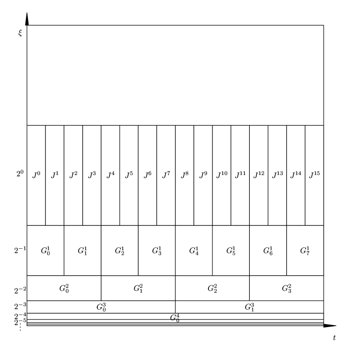
Figure 4.1. $\tilde{X}_{k_{0}}$ norm

Remark 4.19 (Construction of $G_{k}^{j}$ intervals).

For example, in Figure 4.1, we take $k_{0}=4$, $M=2^{k_{0}}=16$, hence there are $16$ small intervals: $J^{0},J^{1},\dots,J^{15}$ at frequency level $2^{0}$. We may treat them as the building blocks in the process of constructing $X$-norm. Then in order to build a lower level $2^{-1}$, we combine every two consecutive small intervals into a larger interval, that is, at a lower level $2^{-1}$, the unions of two consecutive small intervals give us $G_{0}^{1}=J^{0}\cup J^{1},\dots,G_{7}^{1}=J^{14}\cup J^{15}$. Note that upper indices in $G_{k}^{j}$ indicate the length of the time interval (more precisely, $2^{j}$ is the number of small intervals inside $G_{k}^{j}$) and the lower indices in $G_{k}^{j}$ are the locations of the time intervals. In particular, for an interval with its upper indices $0$, it means that it is a $J^{\alpha}$-type small interval, i.e. $G_{k}^{0}=J^{k}$. Then we continue moving onto the next level $2^{-2}$ to get $G_{0}^{2},G_{1}^{2},G_{2}^{2}$ and $G_{3}^{2}$, and even lower levels to get $G_{0}^{3}$, $G_{1}^{3}$ and $G_{0}^{4}$. We can see that $G_{0}^{4}$ is the whole interval $[a,b]$, so we stop building intervals here. For any lever lower than $2^{-4}=2^{k_{0}}$, we just take the whole interval $[a,b]$.

Remark 4.20 (Constriction of the $X$ norm).

We can see the structure of $X$ norm from the figure above. First, we localize the solution $u$ at different frequencies. Then the first term in $X$ norm is:

$$\sum_{i:0\leq i<j}2^{i-j}\sum_{G_{\alpha}^{i}\subset G_{k}^{j}}\operatorname{}\left\|\operatorname{}\left|\nabla\right|^{\frac{1}{2}}P_{2^{-i}}u\right\|_{U_{\Delta}^{2}(G_{\alpha}^{i}\times\mathbb{R}^{2})}^{2}.$$

In fact, for a fixed frequency level $2^{-i}$ (higher than $2^{-j}$), compute the average of frequency localized $U_{\Delta}^{2}$ norms on all the corresponding time intervals $G_{\alpha}^{i}$’s, then sum over all the frequencies higher than $2^{-j}$.

The second term

$$\sum_{i:i\geq j}\operatorname{}\left\|\operatorname{}\left|\nabla\right|^{\frac{1}{2}}P_{2^{-i}}u\right\|_{U_{\Delta}^{2}(G_{k}^{j}\times\mathbb{R}^{2})}^{2}.$$

is the summation of frequency localized $U_{\Delta}^{2}$ norms over all the frequencies lower than $2^{-j}$ on the time interval $G_{k}^{j}$.

Remark 4.21 ($\tilde{X}_{k_{0}}$ norm).

After we compute every $X$ norm over interval $G_{k}^{j}$, we are only two supremums away from the $\tilde{X}_{k_{0}}$ norm on the interval $[a,b]$. First, we fix a frequency level $2^{-j}$ and take the supremum over all the intervals at this level. This step picks out the largest candidates from each level horizontally. Then we choose the largest one from these candidates (vertically). This is the second supremum.

Proposition 4.22 (Some properties of $\tilde{X}_{j}(G_{k}^{j}\times\mathbb{R}^{2})$ norm).

We will use the following estimates in Section 6. For $i\leq j$, let $(q,r)$ be any admissible pair, then we have:

1. $\operatorname{}\left\|\operatorname{}\left|\nabla\right|^{\frac{1}{2}}P_{2^{-i}}u\right\|_{L_{t}^{q}L_{x}^{r}(G_{k}^{j}\times\mathbb{R}^{2})}\lesssim_{q,r}2^{\frac{j-i}{q}}\operatorname{}\left\|u\right\|_{\tilde{X}_{j}(G_{k}^{j}\times\mathbb{R}^{2})}$,

2. $\operatorname{}\left\|P_{>2^{-i}}u\right\|_{L_{t}^{q}L_{x}^{r}(G_{k}^{j}\times\mathbb{R}^{2})}\lesssim 2^{\frac{j}{2}}\operatorname{}\left\|u\right\|_{\tilde{X}_{j}(G_{k}^{j}\times\mathbb{R}^{2})}$,

3. $\operatorname{}\left\|\operatorname{}\left|\nabla\right|^{\frac{1}{2}}P_{\leq 2^{-j}}u\right\|_{L_{t}^{q}L_{x}^{r}(G_{k}^{j}\times\mathbb{R}^{2})}\lesssim\operatorname{}\left\|u\right\|_{\tilde{X}_{j}(G_{k}^{j}\times\mathbb{R}^{2})}$.

Proof.

Similar calculations as in (3.48) and (3.49) in [16], yield Proposition 4.22. ∎

5. Long time Strichartz estimate

In this section, we recall the long time Strichartz estimate introduced in [17] and prove a long time Strichartz estimate adapted in our $\dot{H}^{\frac{1}{2}}$ setting based on the $X_{k_{0}}$ norm defined in Definition 4.18. This long time Strichartz estimate, giving us a good control of low frequency component of the solutions, will be used to in the proof of frequency-localized Morawetz estimates in Section 6.

5.1. Long time Strichartz estimate in the mass-critical regime in two dimensions in [17]

In dimensions two, the endpoint of Strichartz estimates is false, more precisely: Let $P$ be a Fourier multiplier with symbol in $C_{0}^{\infty}(\mathbb{R}^{2})$ (thus $\widehat{Pf}=\phi\hat{f}$ for some $\phi\in C_{0}^{\infty}(\mathbb{R}^{2})$) which is not identically zero. Then there does not exist a constant $C>0$ for which one has the estimate

$$\operatorname{}\left\|e^{it\Delta}Pf\right\|_{L_{t}^{2}L_{x}^{\infty}(\mathbb{R}\times\mathbb{R}^{2})}\leq C\operatorname{}\left\|f\right\|_{L_{x}^{2}(\mathbb{R}^{2})}$$

for all $f\in L_{x}^{2}(\mathbb{R}^{2})$. This makes us unable to choose the regular Strichartz space. However the long time Strichartz estimate highly relies on the double endpoint Strichartz. Therefore, we have to prove new long time Strichartz estimate adapted to two dimensions.

In two dimensional mass-critical regime, Dodson [17] defined a new space on which to compute the long time Strichartz estimates: For any $G_{k}^{j}\subset[a,b]$,

$$\operatorname{}\left\|u\right\|_{X(G_{k}^{j}\times\mathbb{R}^{2})}^{2}:= \sum_{i:0\leq i<j}2^{i-j}\sum_{G_{\alpha}^{i}\subset G_{k}^{j}}\operatorname{}\left\|P_{\xi(G_{\alpha}^{i}),2^{i}}u\right\|_{U_{\Delta}^{2}(G_{\alpha}^{i}\times\mathbb{R}^{2})}^{2}+\sum_{i:i\geq j}\operatorname{}\left\|P_{\xi(G_{k}^{j}),2^{i}}u\right\|_{U_{\Delta}^{2}(G_{k}^{j}\times\mathbb{R}^{2})}^{2}.$$ (5.1)

Then define

$$\operatorname{}\left\|u\right\|_{\tilde{X}_{k_{0}}([a,b]\times\mathbb{R}^{2})}^{2}:=\sup_{j:0\leq j\leq k_{0}}\sup_{G_{k}^{j}\subset[a,b]}\operatorname{}\left\|u\right\|_{X(G_{k}^{j}\times\mathbb{R}^{2})}^{2}.$$

Dodson showed that $\operatorname{}\left\|u\right\|_{\tilde{X}_{k_{0}}([0,T]\times\mathbb{R}^{2})}\lesssim 1$ as the new long time Strichartz estimate in dimensions two, which played a similar role as the long time Strichartz estimate in dimensions three and higher:

$$\operatorname{}\left\|P_{\operatorname{}\left|\xi-\xi(t)\right|>N}u\right\|_{L_{t}^{2}L_{x}^{\frac{2d}{d-2}}(J\times\mathbb{R}^{d})}\lesssim\operatorname{}\left(\frac{K}{N}\right)^{\frac{1}{2}}+1,$$

where $J$ is an interval satisfying

$$\int_{J}N(t)^{3}\,dt=K.$$

5.2. Long time Strichartz estimate and its proof

In contrast to the mass-critical regime, we focus on the low frequency instead of high frequency, and define that for any $G_{k}^{j}\subset[a,b]$,

$$\operatorname{}\left\|u\right\|_{X(G_{k}^{j}\times\mathbb{R}^{2})}^{2}:= \sum_{i:0\leq i<j}2^{i-j}\sum_{G_{\alpha}^{i}\subset G_{k}^{j}}\operatorname{}\left\|\operatorname{}\left|\nabla\right|^{\frac{1}{2}}P_{2^{-i}}u\right\|_{U_{\Delta}^{2}(G_{\alpha}^{i}\times\mathbb{R}^{2})}^{2}+\sum_{i:i\geq j}\operatorname{}\left\|\operatorname{}\left|\nabla\right|^{\frac{1}{2}}P_{2^{-i}}u\right\|_{U_{\Delta}^{2}(G_{k}^{j}\times\mathbb{R}^{2})}^{2}.$$

Then define

$$\operatorname{}\left\|u\right\|_{\tilde{X}_{k_{0}}([a,b]\times\mathbb{R}^{2})}^{2}:=\sup_{j:0\leq j\leq k_{0}}\sup_{G_{k}^{j}\subset[a,b]}\operatorname{}\left\|u\right\|_{X(G_{k}^{j}\times\mathbb{R}^{2})}^{2}.$$

Similarly, we want to show $\operatorname{}\left\|u\right\|_{\tilde{X}_{k_{0}}([0,T]\times\mathbb{R}^{2})}\lesssim 1$, which captures the essential feature in the case that if we assume the double endpoint were true:

$$\operatorname{}\left\|\operatorname{}\left|\nabla\right|^{\frac{1}{2}}P_{<N}u\right\|_{L_{t}^{2}L_{x}^{\infty}(J\times\mathbb{R}^{2})}\lesssim\operatorname{}\left(KN\right)^{\frac{1}{2}}+1,$$

where $J$ is an interval satisfying

$$\int_{J}N(t)\,dt=K.$$

More precisely, we want to show that

Theorem 5.1 (Long time Strichartz estimate).

If $u$ is an almost periodic solution to (1.5) then for any $M=2^{k_{0}}$, $\varepsilon_{1}$, $\varepsilon_{2}$, $\varepsilon_{3}$ satisfying (4.5), $\int_{0}^{T}N(t)\,dt=\varepsilon_{3}M$, and $\int_{0}^{T}\int_{\mathbb{R}^{2}}\operatorname{}\left|u(t,x)\right|^{8}\,dxdt=M$, we have

$$\operatorname{}\left\|u\right\|_{\tilde{X}_{k_{0}}([0,T]\times\mathbb{R}^{2})}^{2}\lesssim 1.$$

Remark 5.2.

Throughout this section the implicit constant depends only on $\operatorname{}\left\|u\right\|_{L_{t}^{\infty}\dot{H}_{x}^{\frac{1}{2}}}$, and not on $M$, or $\varepsilon_{1}$, $\varepsilon_{2}$, $\varepsilon_{3}$.

Proof of Theorem 5.1.

We want to show that for any $0\leq j\leq k$ and $G_{k}^{j}\subset[0,T]$ by induction on $k_{*}$,

$$\sum_{i:0\leq i<j}2^{i-j}\sum_{G_{\alpha}^{i}\subset G_{k}^{j}}\operatorname{}\left\|\operatorname{}\left|\nabla\right|^{\frac{1}{2}}P_{2^{-i}}u\right\|_{U_{\Delta}^{2}(G_{\alpha}^{i}\times\mathbb{R}^{2})}^{2}+\sum_{i:i\geq j}\operatorname{}\left\|\operatorname{}\left|\nabla\right|^{\frac{1}{2}}P_{2^{-i}}u\right\|_{U_{\Delta}^{2}(G_{k}^{j}\times\mathbb{R}^{2})}^{2}\lesssim 1.$$

5.2.1. Base case

First, we start with the base case ($k_{*}=0$), that is, $\operatorname{}\left\|u\right\|_{\tilde{X}_{0}([0,T]\times\mathbb{R}^{2})}\lesssim 1$.

Let $J^{\alpha}=[a_{\alpha},b_{\alpha}]$. By the integral equation, Strichartz estimates, duality (Proposition 4.7), $V_{\Delta}^{2}\hookrightarrow U_{\Delta}^{4}\hookrightarrow L_{t}^{4}L_{x}^{4}$ (Theorem 4.5), Definition 4.12, and Remark 4.14, we write

$$\operatorname{}\left\|\operatorname{}\left|\nabla\right|^{\frac{1}{2}}u\right\|_{U_{\Delta}^{2}(J^{\alpha}\times\mathbb{R}^{2})} \lesssim\operatorname{}\left\|u\right\|_{L_{t}^{\infty}\dot{H}^{\frac{1}{2}}(J^{\alpha}\times\mathbb{R}^{2})}+\sup_{\operatorname{}\left\|v\right\|_{V_{\Delta}^{2}}=1}\int_{J^{\alpha}}\operatorname{}\left\langle v,\operatorname{}\left|\nabla\right|^{\frac{1}{2}}F(u)\right\rangle\,dt\lesssim 1.$$

To compute $\operatorname{}\left\|u\right\|_{X(J^{\alpha}\times\mathbb{R}^{2})}$, we know that at the base case level, the only small interval inside a small interval $J^{\alpha}$ is itself, hence we have no first term in (4.6). Then by Definition 4.18, Littlewood-Paley theorem, Minkowski, Hölder and Remark 4.14, we obtain

$$\operatorname{}\left\|u\right\|_{X(J^{\alpha}\times\mathbb{R}^{2})}^{2} \lesssim\sum_{i:i\geq 0}\operatorname{}\left(\operatorname{}\left\|\operatorname{}\left|\nabla\right|^{\frac{1}{2}}P_{2^{-i}}u(a_{\alpha})\right\|_{L_{x}^{2}}^{2}+\operatorname{}\left\|\operatorname{}\left|\nabla\right|^{\frac{1}{2}}P_{2^{-i}}F(u)\right\|_{L_{t}^{1}L_{x}^{2}(J^{\alpha}\times\mathbb{R}^{2})}^{2}\right)\lesssim 1.$$

Note that when $k_{\ast}=0$, the supremum of (4.6) over all intervals $G_{k}^{j}\subset[0,T]$ becomes the the supremum of over all small intervals $J^{\alpha}\subset[0,T]$. Therefore, by Definition 4.18,

$$\operatorname{}\left\|u\right\|_{\tilde{X}_{0}([0,T]\times\mathbb{R}^{2})}^{2}=\sup_{j=0}\sup_{J^{\alpha}\subset[0,T]}\operatorname{}\left\|u\right\|_{X(J^{\alpha}\times\mathbb{R}^{2})}^{2}\leq C(u).$$ (5.2)

Notice that $C(u)$ only depends on $\operatorname{}\left\|u\right\|_{L_{t}^{\infty}\dot{H}^{\frac{1}{2}}[0,T]\times\mathbb{R}^{2}}$.

5.2.2. Induction

By Definition 4.18, Lemma 4.6, we have

$$\operatorname{}\left\|u\right\|_{\tilde{X}_{k_{\ast}+1}([0,T]\times\mathbb{R}^{2})}^{2}\leq 2\operatorname{}\left\|u\right\|_{\tilde{X}_{k_{\ast}}([0,T]\times\mathbb{R}^{2})}^{2}.$$ (5.3)

Therefore, by (5.2) and (5.3),

$$\operatorname{}\left\|u\right\|_{\tilde{X}_{11}([0,T]\times\mathbb{R}^{2})}^{2}\leq 2^{11}C(u).$$ (5.4)

5.2.3. Bootstrap

For $j>11$ and $G_{k}^{j}\subset[0,T]$, we want to prove that $\operatorname{}\left\|u\right\|_{\tilde{X}_{j}(G_{k}^{j}\times\mathbb{R}^{2})}\leq 2^{11}C(u)$ by bootstrap argument.

First consider the terms in the $X$ norm in (4.6) with frequencies localized higher than $2^{-11}$, and they are bounded due to (5.4) (see Step 1). For the terms in the $X$ norm with frequencies localized lower than $2^{-11}$, we can use the integral equation to rewrite $u$ into the free solution and the Duhamel term, then compute the contributions of these two terms to the first term (A) and the second term (B) of the $X$ norm respectively. As a result, we have a free solution term (AF) and a Duhamel term (AD) contributing to A, and a free solution term (BF) and a Duhamel term (BD) contributing to B.

$$X(G_{k}^{j})\text{ norm }\begin{cases}\text{frequencies higher than }2^{-11}\text{ (Step 1)}\\ \text{frequencies lower than }2^{-11}\begin{cases}\text{1st term }A\begin{cases}\text{free solution }AF\text{ (Step 2)}\\ \text{Duhamel term }AD\text{ (Step 4)}\end{cases}\\ \text{2nd term }B\begin{cases}\text{free solution }BF\text{ (Step 3)}\\ \text{Duhamel term }BD\text{ (Step 4)}\end{cases}\end{cases}\end{cases}$$

We will consider the terms with frequencies higher than $2^{-11}$ in Step 1. And estimates the free solution terms in A and B in Step 2 and Step 3 respectively. In this proof, the hardest part is to estimate AD and BD. We will bound them in Step 4.

It is worth mentioning that in Step 4, we treat two different types of $G_{\alpha}^{i}$ intervals in two cases (see the classification of these two cases in Step 4). For case 1, we compute directly, while for case 2, we will prove a bootstrap argument Proposition 5.3. In the proof we decompose the nonlinear term $\operatorname{}\left|u\right|^{4}u$ into different frequencies and consider them in Lemma 5.4 and Lemma 5.5.

$$\text{Step 4 }(AD\,\&\,BD)\to\begin{cases}\text{case 1}\\ \text{case 2}\to\text{Proposition \ref{prop Term 1&2}}\begin{cases}\text{Lemma \ref{lem Term1}}\\ \text{Lemma \ref{lem Term2}}\end{cases}\end{cases}$$

Step 1: Frequencies higher than $2^{-11}$

Note that $G_{j}^{k}$ overlaps $2^{j-11}$ intervals $G_{\beta}^{11}$ and $G_{\beta}^{11}$ overlaps $2^{11-i}$ intervals $G_{\alpha}^{i}$. So by Fubini-Tonelli theorem, (5.4) implies that for any $j>11$ and $G_{k}^{j}\subset[0,T]$,

$$\sum_{i:0\leq i\leq 11}2^{i-j}\sum_{G_{\alpha}^{i}\subset G_{k}^{j}}\operatorname{}\left\|\operatorname{}\left|\nabla\right|^{\frac{1}{2}}P_{2^{-i}}u\right\|_{U_{\Delta}^{2}(G_{\alpha}^{i}\times\mathbb{R}^{2})}^{2}\leq 2^{11}C(u).$$

Step 2: Free solution term in A

Fix $k_{0}$, $12\leq j\leq k_{0}$, and $G_{k}^{j}\subset[0,T]$. For $11\leq i<j$, Duhamel’s principle implies

$$\operatorname{}\left\|\operatorname{}\left|\nabla\right|^{\frac{1}{2}}P_{2^{-i}}u\right\|_{U_{\Delta}^{2}(G_{\alpha}^{i}\times\mathbb{R}^{2})}\lesssim\operatorname{}\left\|\operatorname{}\left|\nabla\right|^{\frac{1}{2}}P_{2^{-i}}u(t_{\alpha}^{i})\right\|_{L_{x}^{2}(\mathbb{R}^{2})}+\operatorname{}\left\|\operatorname{}\left|\nabla\right|^{\frac{1}{2}}\int_{t_{\alpha}^{i}}^{t}e^{i(t-t^{\prime})\Delta}P_{2^{-i}}F(u)\,dt^{\prime}\right\|_{U_{\Delta}^{2}(G_{\alpha}^{i}\times\mathbb{R}^{2})}.$$

Choose $t_{\alpha}^{i}$ satisfying

$$\operatorname{}\left\|\operatorname{}\left|\nabla\right|^{\frac{1}{2}}P_{2^{-i}}u(t_{\alpha}^{i})\right\|_{L_{x}^{2}(\mathbb{R}^{2})}=\inf_{t\in G_{\alpha}^{i}}\operatorname{}\left\|\operatorname{}\left|\nabla\right|^{\frac{1}{2}}P_{2^{-i}}u(t)\right\|_{L_{x}^{2}(\mathbb{R}^{2})}.$$ (5.5)

Then by Definition 4.12, Fubini-Tonelli theorem and (5.5),

$$\quad\sum_{i:11\leq i<j}2^{i-j}\sum_{G_{\alpha}^{i}\subset G_{k}^{j}}\operatorname{}\left\|\operatorname{}\left|\nabla\right|^{\frac{1}{2}}P_{2^{-i-2}\leq\cdot\leq 2^{-i+2}}u(t_{\alpha}^{i})\right\|_{L_{x}^{2}(\mathbb{R}^{2})}^{2}$$

$$\leq\frac{1}{2\varepsilon_{3}}2^{-j}\sum_{G_{\alpha}^{i}\subset G_{k}^{j}}\int_{G_{\alpha}^{i}}\sum_{i:11\leq i<j}\operatorname{}\left\|\operatorname{}\left|\nabla\right|^{\frac{1}{2}}P_{2^{-i}}u(t)\right\|_{L_{x}^{2}(\mathbb{R}^{2})}^{2}\operatorname{}\left(\varepsilon_{3}\operatorname{}\left\|u(t)\right\|_{L_{x}^{8}(\mathbb{R}^{2})}^{8}+N(t)\right)\,dt\lesssim 1.$$

Step 3: Free solution term in B

For $i\geq j$ simply take $t_{0}$, where $t_{0}$ is a fixed element of $G_{k}^{j}$, say the left endpoint. Then

$$\sum_{i:i\geq j}\operatorname{}\left\|\operatorname{}\left|\nabla\right|^{\frac{1}{2}}P_{2^{-i}}e^{it\Delta}u(t_{0})\right\|_{U_{\Delta}^{2}(G_{k}^{j}\times\mathbb{R}^{2})}^{2}\lesssim\sum_{i:i\geq j}\operatorname{}\left\|\operatorname{}\left|\nabla\right|^{\frac{1}{2}}P_{2^{-i}}u(t_{0})\right\|_{L_{x}^{2}(\mathbb{R}^{2})}^{2}\lesssim 1.$$

Therefore, from Step 2 and Step 3, we have the following bound for the free solution terms AF and BF:

$$\sum_{i:0\leq i<j}2^{i-j}\sum_{G_{\alpha}^{i}\subset G_{k}^{j}}\operatorname{}\left\|\operatorname{}\left|\nabla\right|^{\frac{1}{2}}P_{2^{-i}}u\right\|_{L_{x}^{2}(\mathbb{R}^{2})}^{2}+\sum_{i:i\geq j}\operatorname{}\left\|\operatorname{}\left|\nabla\right|^{\frac{1}{2}}P_{2^{-i}}u\right\|_{L_{x}^{2}(\mathbb{R}^{2})}^{2}\lesssim 1.$$

Thanks to the calculation above, we have

$$\operatorname{}\left\|u\right\|_{X(G_{k}^{j}\times\mathbb{R}^{2})}^{2} \lesssim 1+\sum_{i:11\leq i<j}2^{i-j}\sum_{G_{\alpha}^{i}\subset G_{k}^{j}}\operatorname{}\left\|\operatorname{}\left|\nabla\right|^{\frac{1}{2}}\int_{t_{\alpha}^{i}}^{t}e^{i(t-t^{\prime})\Delta}P_{2^{-i}}F(u)\,dt^{\prime}\right\|_{U_{\Delta}^{2}(G_{\alpha}^{i}\times\mathbb{R}^{2})}^{2}$$

$$+\sum_{i:i\geq j}\operatorname{}\left\|\operatorname{}\left|\nabla\right|^{\frac{1}{2}}\int_{t_{0}}^{t}e^{i(t-t^{\prime})\Delta}P_{2^{-i}}F(u)\,dt^{\prime}\right\|_{U_{\Delta}^{2}(G_{k}^{j}\times\mathbb{R}^{2})}^{2}.$$

Step 4: Duhamel terms in A and B

For these two terms, we consider the intervals $G_{\alpha}^{i}$ and $G_{k}^{j}$ in the following cases:

$$\begin{cases}\text{Case 1 : }G_{\alpha}^{i}:G_{\alpha}^{i}\subset G_{k}^{j}\text{ and }N(G_{\alpha}^{i})\leq\varepsilon_{3}^{-1/2}2^{-i};\text{ and }G_{k}^{j}:N(G_{k}^{j})\leq\varepsilon_{3}^{-1/2}2^{-j},\\ \text{Case 2 : }G_{\alpha}^{i}:G_{\alpha}^{i}\subset G_{k}^{j}\text{ and }N(G_{\alpha}^{i})\geq\varepsilon_{3}^{-1/2}2^{-i};\text{ and }G_{k}^{j}:N(G_{k}^{j})\geq\varepsilon_{3}^{-1/2}2^{-j}.\end{cases}$$

$\bullet$ Case 1 in Step 4: There are at most two small intervals, call them $J_{1}$ and $J_{2}$, that intersect $G_{k}^{j}$ but are not contained in $G_{k}^{j}$. Therefore, by Minkowski, Hölder and Remark 4.14

$$\sum_{i:11\leq i<j}2^{i-j}\sum_{G_{\alpha}^{i}\subset G_{k}^{j}}\operatorname{}\left\|\operatorname{}\left|\nabla\right|^{\frac{1}{2}}F(u)\right\|_{L_{t}^{1}L_{x}^{2}(G_{\alpha}^{i}\cap(J_{1}\cup J_{2})\times\mathbb{R}^{2})}^{2} \lesssim\sum_{i:11\leq i<j}2^{i-j}\operatorname{}\left\|\operatorname{}\left|\nabla\right|^{\frac{1}{2}}F(u)\right\|_{L_{t}^{1}L_{x}^{2}(J_{1}\cup J_{2}\times\mathbb{R}^{2})}^{2}\lesssim 1$$ (5.6)

Next observe that $N(G_{\alpha}^{i})\leq\varepsilon_{3}^{-1/2}2^{-i}$ implies that $N(t)\leq\varepsilon_{3}^{-1/2}2^{-i+1}$ for all $t\in G_{\alpha}^{i}$. In fact, by Remark 4.17 the difference of $\frac{1}{N(t)}$ on $G_{\alpha}^{i}$ is at most $\varepsilon_{1}^{-1/2}\varepsilon_{3}2^{i}$, hence

$$N(t)\leq N(G_{\alpha}^{i})+\varepsilon_{1}^{-1/2}\varepsilon_{3}2^{i}\leq\varepsilon_{3}^{-1/2}2^{-i+1}\quad\text{ for all }t\in G_{\alpha}^{i}.$$

Now by Definition 4.11 and Definition 4.12, the number of $J_{l}$ intervals inside $G_{\alpha}^{i}$ is

$$\#\{J_{l}:J_{l}\subset G_{\alpha}^{i}\}\sim\int_{\cup J_{l}}N(t)^{2}\,dt\lesssim\int_{G_{\alpha}^{i}}N(t)^{2}\,dt\leq\varepsilon_{3}^{-1/2}2^{-i+1}\int_{G_{\alpha}^{i}}N(t)\,dt\leq\varepsilon_{3}^{1/2}2^{2}.$$

This implies that the number of intervals $J_{l}$ such that $N(t)\leq\varepsilon_{3}^{-1/2}2^{-i+1}$ for all $t\in G_{\alpha}^{i}$ is finite and does not depend on $G_{\alpha}^{i}$. By (5.6), Fubini-Tonelli theorem and Remark 4.16, we have

$$\quad\sum_{i:11\leq i<j}2^{i-j}\sum_{\begin{subarray}{c}G_{\alpha}^{i}\subset G_{k}^{j}\\ N(G_{\alpha}^{i})\leq\varepsilon_{3}^{-1/2}2^{-i}\end{subarray}}\operatorname{}\left\|\operatorname{}\left|\nabla\right|^{\frac{1}{2}}\int_{t_{\alpha}^{i}}^{t}e^{i(t-t^{\prime})\Delta}P_{2^{-i}}F(u)\,dt^{\prime}\right\|_{U_{\Delta}^{2}(G_{\alpha}^{i}\times\mathbb{R}^{2})}^{2}$$

$$\lesssim\sum_{i:11\leq i<j}2^{i-j}\sum_{G_{\alpha}^{i}\subset G_{k}^{j}}\operatorname{}\left\|\operatorname{}\left|\nabla\right|^{\frac{1}{2}}F(u)\right\|_{L_{t}^{1}L_{x}^{2}(G_{\alpha}^{i}\cap(J_{1}\cup J_{2})\times\mathbb{R}^{2})}^{2}$$

$$+\sum_{i:11\leq i<j}2^{i-j}\sum_{\begin{subarray}{c}J_{l}\subset G_{k}^{j}\\ N(J_{l})\leq\varepsilon_{3}^{-1/2}2^{-i+1}\end{subarray}}\operatorname{}\left\|\operatorname{}\left|\nabla\right|^{\frac{1}{2}}F(u)\right\|_{L_{t}^{1}L_{x}^{2}(J_{l}\times\mathbb{R}^{2})}^{2}\lesssim 1$$

Similarly, if $N(G_{k}^{j})\leq\varepsilon_{3}^{-1/2}2^{-j}$, then $N(t)\leq\varepsilon_{3}^{-1/2}2^{-j+1}$ for all $t\in G_{k}^{j}$. This implies that

$$\operatorname{}\left\|u\right\|_{L_{t}^{8}L_{x}^{8}(G_{k}^{j}\times\mathbb{R}^{2})}^{8}\sim\int_{G_{k}^{j}}N(t)^{2}\,dt\leq\varepsilon_{3}^{-1/2}2^{-j+1}\int_{G_{k}^{j}}N(t)\,dt\leq\varepsilon_{3}^{-1/2}2^{-j+1}\varepsilon_{3}2^{j}\lesssim 1.$$

Hence,

$$\operatorname{}\left\|\operatorname{}\left|\nabla\right|^{\frac{1}{2}}u\right\|_{L_{t}^{q}L_{x}^{r}(G_{k}^{j}\times\mathbb{R}^{2})}\lesssim 1\quad\text{ for any admissible pair }(q,r).$$ (5.7)

Therefore, by Minkowski and Hölder and (5.7)

$$\sum_{\begin{subarray}{c}i:i\geq j\\ N(G_{k}^{j})\leq\varepsilon_{3}^{-1/2}2^{-j}\end{subarray}}\operatorname{}\left\|\operatorname{}\left|\nabla\right|^{\frac{1}{2}}P_{2^{-i}}F(u)\right\|_{L_{t}^{1}L_{x}^{2}(G_{k}^{j}\times\mathbb{R}^{2})}^{2}\lesssim\operatorname{}\left\|\operatorname{}\left|\nabla\right|^{\frac{1}{2}}P_{\leq 2^{-j+2}}F(u)\right\|_{L_{t}^{1}L_{x}^{2}(G_{k}^{j}\times\mathbb{R}^{2})}^{2}\lesssim 1.$$

Therefore, all the computation above yields

$$\operatorname{}\left\|u\right\|_{X(G_{k}^{j}\times\mathbb{R}^{2})}^{2} \lesssim 1+\sum_{i;11\leq i<j}2^{i-j}\sum_{\begin{subarray}{c}G_{\alpha}^{i}\subset G_{k}^{j}\\ N(G_{\alpha}^{i})\geq\varepsilon_{3}^{-1/2}2^{-i}\end{subarray}}\operatorname{}\left\|\operatorname{}\left|\nabla\right|^{\frac{1}{2}}\int_{t_{\alpha}^{i}}^{t}e^{i(t-t^{\prime})\Delta}P_{2^{-i}}F(u)\,dt^{\prime}\right\|_{U_{\Delta}^{2}(G_{\alpha}^{i}\times\mathbb{R}^{2})}^{2}$$

$$+\sum_{\begin{subarray}{c}i:i\geq j\\ N(G_{k}^{j})\geq\varepsilon_{3}^{-1/2}2^{-j}\end{subarray}}\operatorname{}\left\|\operatorname{}\left|\nabla\right|^{\frac{1}{2}}\int_{t_{0}}^{t}e^{i(t-t^{\prime})\Delta}P_{2^{-i}}F(u)\,dt^{\prime}\right\|_{U_{\Delta}^{2}(G_{k}^{j}\times\mathbb{R}^{2})}^{2}.$$ (5.8)

$\bullet$ Case 2 in Step 4: From now on, we take the intervals $G_{\alpha}^{i}$ with $N(G_{\alpha}^{i})\geq\varepsilon_{3}^{-1/2}2^{-i}$ and the intervals $G_{k}^{j}$ with $N(G_{k}^{j})\geq\varepsilon_{3}^{-1/2}2^{-j}$. Continue from (5.2.3). To close the proof of the long time Strichartz, it suffices to prove the following proposition:

Proposition 5.3.

$$\quad\sum_{i:11\leq i<j}2^{i-j}\sum_{\begin{subarray}{c}G_{\alpha}^{i}\subset G_{k}^{j}\\ N(G_{\alpha}^{i})\geq\varepsilon_{3}^{-1/2}2^{-i}\end{subarray}}\operatorname{}\left\|\operatorname{}\left|\nabla\right|^{\frac{1}{2}}\int_{t_{\alpha}^{i}}^{t}e^{i(t-t^{\prime})\Delta}P_{2^{-i}}F(u)\,dt^{\prime}\right\|_{U_{\Delta}^{2}(G_{\alpha}^{i}\times\mathbb{R}^{2})}^{2}$$ (5.9)

$$+\sum_{\begin{subarray}{c}i:i\geq j\\ N(G_{k}^{j})\geq\varepsilon_{3}^{-1/2}2^{-j}\end{subarray}}\operatorname{}\left\|\operatorname{}\left|\nabla\right|^{\frac{1}{2}}\int_{t_{0}}^{t}e^{i(t-t^{\prime})\Delta}P_{2^{-i}}F(u)\,dt^{\prime}\right\|_{U_{\Delta}^{2}(G_{k}^{j}\times\mathbb{R}^{2})}^{2}$$

$$\lesssim\varepsilon_{2}^{4}\operatorname{}\left\|u\right\|_{\tilde{X}_{j}([0,T]\times\mathbb{R}^{2})}^{6}+\varepsilon_{2}^{2}\operatorname{}\left\|u\right\|_{\tilde{X}_{j}([0,T]\times\mathbb{R}^{2})}^{8}.$$

Indeed, assuming that Proposition 5.3 is true, we can run a bootstrap argument.

Suppose

$$\operatorname{}\left\|u\right\|_{\tilde{X}_{k_{*}}([0,T]\times\mathbb{R}^{2})}^{2}\leq C_{0}.$$ (5.10)

Then by (5.3)

$$\operatorname{}\left\|u\right\|_{\tilde{X}_{k_{*}+1}([0,T]\times\mathbb{R}^{2})}^{2}\leq 2C_{0}.$$

Then by (5.2.3) and Proposition 5.3, we have

$$\operatorname{}\left\|u\right\|_{\tilde{X}_{k_{*}+1}([0,T]\times\mathbb{R}^{2})}^{2}\leq C(u)\operatorname{}\left(1+\varepsilon_{2}^{4}(2C_{0})^{3}+\varepsilon_{2}^{2}(2C_{0})^{4}\right).$$

Taking $C_{0}=2^{11}C(u)$ and $\varepsilon_{2}>0$ sufficiently small, it implies that (5.10) holds for $k_{*}=11$. The bootstrap argument is closed, since we obtain

$$\operatorname{}\left\|u\right\|_{\tilde{X}_{k_{*}+1}([0,T]\times\mathbb{R}^{2})}^{2}\leq C_{0}.$$

Hence the long time Strichartz estimates follow by (5.2), (5.3) and induction on $k_{*}$.

Now we are left to show Proposition 5.3.

Proof of Proposition 5.3.

We first write $F(u)$ into the Littlewood-Paley decomposition. Without loss of generality, we assume that $2^{-n_{1}}\geq 2^{-n_{2}}\geq 2^{-n_{3}}\geq 2^{-n_{4}}\geq 2^{-n_{5}}$, i.e. $n_{1}\leq n_{2}\leq n_{3}\leq n_{4}\leq n_{5}$. In the proof, since we utilize Lebesgue norms $L_{x}^{q}L_{x}^{r}$ and Lebesgue norms do not see the difference between $u$ and $\bar{u}$, i.e, $\operatorname{}\left\|P_{N}u\right\|_{L_{x}^{q}L_{x}^{r}}=\operatorname{}\left\|P_{N}\bar{u}\right\|_{L_{x}^{q}L_{x}^{r}}$, it is safe for us to write

$$P_{2^{-i}}F(u)\simeq P_{2^{-i}}\operatorname{}\left(\sum_{n_{1}\leq n_{2}\leq n_{3}\leq n_{4}\leq n_{5}}f\right)$$

where $f=(P_{2^{-n_{1}}}u)(P_{2^{-n_{2}}}u)(P_{2^{-n_{3}}}u)(P_{2^{-n_{4}}}u)(P_{2^{-n_{5}}}u)$.

Then we compare the largest frequency $2^{-n_{1}}$ with $2^{-i}$:

• If $2^{-i}\gg 2^{-n_{1}}$, it is impossible since $P_{2^{-i}}((P_{\leq 2^{-i-7}}u)^{5})=0$;

• If $2^{-i}\sim 2^{-n_{1}}$(i.e. $2^{-n_{1}-7}\leq 2^{-i}\leq 2^{-n_{1}+7}$), then this is our fist case:

  $$2^{-i}\sim 2^{-n_{1}}\geq 2^{-n_{2}}\geq 2^{-n_{3}}\geq 2^{-n_{4}}\geq 2^{-n_{5}};$$

• If $2^{-i}\ll 2^{-n_{1}}$, then $2^{-n_{2}}$ must have a similar frequency with $2^{-n_{1}}$, otherwise the projection to $2^{-i}$ frequency of this term will be zero. Hence the second case is

  $$2^{-i}\leq 2^{-n_{1}}\sim 2^{-n_{2}};2^{-n_{1}}\geq 2^{-n_{2}}\geq 2^{-n_{3}}\geq 2^{-n_{4}}\geq 2^{-n_{5}}.$$

Therefore, it is sufficient to consider the following:

$$P_{2^{-i}}F(u) \simeq P_{2^{-i}}\operatorname{}\left(\sum_{\begin{subarray}{c}n_{1}\sim i;\\ n_{1}\leq n_{2}\leq n_{3}\leq n_{4}\leq n_{5}\end{subarray}}f\right)+P_{2^{-i}}\operatorname{}\left(\sum_{\begin{subarray}{c}n_{1}<i;n_{1}\sim n_{2};\\ n_{1}\leq n_{2}\leq n_{3}\leq n_{4}\leq n_{5}\end{subarray}}f\right):=\tilde{F}_{1}+\tilde{F}_{2}.$$

Next, we compute the contributions of $\tilde{F}_{1}$ and $\tilde{F}_{2}$ to (5.9) in Lemma 5.4 and Lemma 5.5 respectively.

Lemma 5.4 (Contribution of $\tilde{F}_{1}$).

For a fixed $G_{k}^{j}\subset[0,T]$, $j>11$,

$$\sum_{i:11\leq i<j}2^{i-j}\sum_{\begin{subarray}{c}G_{\alpha}^{i}\subset G_{k}^{j}\\ N(G_{\alpha}^{i})\geq\varepsilon_{3}^{-1/2}2^{-i}\end{subarray}}\operatorname{}\left\|\operatorname{}\left|\nabla\right|^{\frac{1}{2}}\int_{t_{\alpha}^{i}}^{t}e^{i(t-t^{\prime})\Delta}\tilde{F}_{1}\,dt^{\prime}\right\|_{U_{\Delta}^{2}(G_{\alpha}^{i}\times\mathbb{R}^{2})}^{2}$$ (5.11)

$$+\sum_{\begin{subarray}{c}i:i\geq j\\ N(G_{k}^{j})\geq\varepsilon_{3}^{-1/2}2^{-j}\end{subarray}}\operatorname{}\left\|\operatorname{}\left|\nabla\right|^{\frac{1}{2}}\int_{t_{0}}^{t}e^{i(t-t^{\prime})\Delta}\tilde{F}_{1}\,dt^{\prime}\right\|_{U_{\Delta}^{2}(G_{k}^{j}\times\mathbb{R}^{2})}^{2}$$ (5.12)

$$\lesssim\varepsilon_{2}^{4}\operatorname{}\left\|u\right\|_{\tilde{X}_{j}([0,T]\times\mathbb{R}^{2})}^{6}.$$

Proof.

By Proposition 4.7,

$$\quad\operatorname{}\left\|\operatorname{}\left|\nabla\right|^{\frac{1}{2}}\int_{t_{\alpha}^{i}}^{t}e^{i(t-t^{\prime})\Delta}\tilde{F}_{1}\,dt^{\prime}\right\|_{U_{\Delta}^{2}(G_{\alpha}^{i}\times\mathbb{R}^{2})}\lesssim\sup_{\operatorname{}\left\|v\right\|_{V_{\Delta}^{2}(G_{\alpha}^{i}\times\mathbb{R}^{2})}=1}\int_{G_{\alpha}^{i}}\operatorname{}\left\langle v,\operatorname{}\left|\nabla\right|^{\frac{1}{2}}\tilde{F}_{1}\right\rangle\,dt$$

$$\lesssim\sum_{\begin{subarray}{c}n_{1}\sim i;\\ n_{1}\leq n_{2}\leq n_{3}\leq n_{4}\leq n_{5}\end{subarray}}\sup_{\operatorname{}\left\|v\right\|_{V_{\Delta}^{2}(G_{\alpha}^{i}\times\mathbb{R}^{2})}=1}\int_{G_{\alpha}^{i}}\operatorname{}\left\langle\operatorname{}\left|\nabla\right|^{\frac{1}{2}}P_{2^{-i}}v,f\right\rangle\,dt.$$ (5.13)

Lemma 1.11 implies that $N(t)$ is bounded on $G_{\alpha}^{i}$, and recall $N(G_{\alpha}^{i})=\inf_{t\in G_{\alpha}^{i}}N(t)$, $2^{-n_{5}}\leq 2^{-n_{4}}\leq\varepsilon_{3}^{1/2}N(t)$ and (4.5), we know that

$$\operatorname{}\left\|P_{2^{-n_{4}}}u\right\|_{L_{t}^{\infty}L_{x}^{4}(G_{\alpha}^{i}\times\mathbb{R}^{2})}\lesssim\varepsilon_{2},\quad\operatorname{}\left\|P_{2^{-n_{5}}}u\right\|_{L_{t}^{\infty}L_{x}^{4}(G_{\alpha}^{i}\times\mathbb{R}^{2})}\lesssim\varepsilon_{2}.$$ (5.14)

Then using Hölder and Bernstein, we write

$$\int_{G_{\alpha}^{i}}\operatorname{}\left\langle\operatorname{}\left|\nabla\right|^{\frac{1}{2}}P_{2^{-i}}v,f\right\rangle\,dt\lesssim 2^{-\frac{i}{2}}\operatorname{}\left\|v\right\|_{L_{t}^{4}L_{x}^{4}(G_{\alpha}^{i}\times\mathbb{R}^{2})}\operatorname{}\left\|P_{2^{-n_{1}}}u\right\|_{L_{t}^{4}L_{x}^{4}(G_{\alpha}^{i}\times\mathbb{R}^{2})}\operatorname{}\left\|P_{2^{-n_{2}}}u\right\|_{L_{t}^{4}L_{x}^{4}(G_{\alpha}^{i}\times\mathbb{R}^{2})}$$

$$\times\operatorname{}\left\|P_{2^{-n_{3}}}u\right\|_{L_{t}^{4}L_{x}^{4}(G_{\alpha}^{i}\times\mathbb{R}^{2})}\operatorname{}\left\|P_{2^{-n_{4}}}u\right\|_{L_{t}^{\infty}L_{x}^{\infty}(G_{\alpha}^{i}\times\mathbb{R}^{2})}\operatorname{}\left\|P_{2^{-n_{5}}}u\right\|_{L_{t}^{\infty}L_{x}^{\infty}(G_{\alpha}^{i}\times\mathbb{R}^{2})}.$$ (5.15)

By $V_{\Delta}^{2}\hookrightarrow U_{\Delta}^{4}$ (Theorem 4.5), Bernstein, (5.14) and (5.15), then (5.13) becomes

$$\eqref{eq5 Thm LTS} \lesssim\sum_{\begin{subarray}{c}n_{1}\sim i;\\ n_{1}\leq n_{2}\leq n_{3}\leq n_{4}\leq n_{5}\end{subarray}}2^{\frac{n_{1}}{2}-\frac{i}{2}+\frac{n_{2}}{2}+\frac{n_{3}}{2}-\frac{n_{4}}{2}-\frac{n_{5}}{2}}\operatorname{}\left\|\operatorname{}\left|\nabla\right|^{\frac{1}{2}}P_{2^{-n_{1}}}u\right\|_{U_{\Delta}^{2}(G_{\alpha}^{i}\times\mathbb{R}^{2})}$$

$$\qquad\times\operatorname{}\left\|\operatorname{}\left|\nabla\right|^{\frac{1}{2}}P_{2^{-n_{2}}}u\right\|_{U_{\Delta}^{2}(G_{\alpha}^{i}\times\mathbb{R}^{2})}\operatorname{}\left\|\operatorname{}\left|\nabla\right|^{\frac{1}{2}}P_{2^{-n_{3}}}u\right\|_{U_{\Delta}^{2}(G_{\alpha}^{i}\times\mathbb{R}^{2})}\varepsilon_{2}^{2}.$$ (5.16)

The sum over $n_{2}$, $n_{3}$, $n_{4}$ and $n_{5}$ in (5.16) of the component depending only on these frequencies is bounded by a multiple of $\operatorname{}\left\|u\right\|_{\tilde{X}_{j}([0,T]\times\mathbb{R}^{2})}^{2}$. The sum over $n_{1}$ in (5.16) is in fact a finite sum. Combining (5.13), (5.16), Definition 4.18 and the fact that the number of $G_{\alpha}^{i}$ such that $G_{\alpha}^{i}\subset G_{k}^{j}$ is at most $2^{7}$ , we have

$$\eqref{eq Term1 lem term1} \lesssim\sum_{i:11\leq i<j}2^{i-j}\sum_{\begin{subarray}{c}G_{\alpha}^{i}\subset G_{k}^{j}\\ N(G_{\alpha}^{i})\geq\varepsilon_{3}^{-1/2}2^{-i}\end{subarray}}\sum_{n_{1}:n_{1}\sim i}2^{n_{1}-i}\operatorname{}\left\|\operatorname{}\left|\nabla\right|^{\frac{1}{2}}P_{2^{-n_{1}}}u\right\|_{U_{\Delta}^{2}(G_{\alpha}^{i}\times\mathbb{R}^{2})}^{2}\operatorname{}\left\|u\right\|_{\tilde{X}_{j}([0,T]\times\mathbb{R}^{2})}^{4}\varepsilon_{2}^{4}$$

$$\lesssim\varepsilon_{2}^{4}\operatorname{}\left\|u\right\|_{\tilde{X}_{j}([0,T]\times\mathbb{R}^{2})}^{6}$$

Similarly, the second term (5.12) in Lemma 5.4 becomes,

$$\eqref{eq Term2 lem term1} \lesssim\sum_{\begin{subarray}{c}i:i\geq j\\ N(G_{k}^{j})\geq\varepsilon_{3}^{-1/2}2^{-j}\end{subarray}}\operatorname{}\left\|\operatorname{}\left|\nabla\right|^{\frac{1}{2}}P_{2^{-i}}u\right\|_{U_{\Delta}^{2}(G_{k}^{j}\times\mathbb{R}^{2})}^{2}\varepsilon_{3}^{4}\operatorname{}\left\|u\right\|_{\tilde{X}_{j}([0,T]\times\mathbb{R}^{2})}^{4}\lesssim\varepsilon_{2}^{4}\operatorname{}\left\|u\right\|_{\tilde{X}_{j}([0,T]\times\mathbb{R}^{2})}^{6}.$$

Therefore, the proof of Lemma 5.4 is complete. ∎

Next, we estimate the contribution of $\tilde{F}_{2}$ in the decomposition in Proposition 5.3.

Lemma 5.5 (Contribution of $\tilde{F}_{2}$).

For a fixed $G_{k}^{j}\subset[0,T]$, $j>11$,

$$\quad\sum_{i:11\leq i<j}2^{i-j}\sum_{\begin{subarray}{c}G_{\alpha}^{i}\subset G_{k}^{j}\\ N(G_{\alpha}^{i})\geq\varepsilon_{3}^{-1/2}2^{-i}\end{subarray}}\operatorname{}\left\|\operatorname{}\left|\nabla\right|^{\frac{1}{2}}\int_{t_{\alpha}^{i}}^{t}e^{i(t-t^{\prime})\Delta}\tilde{F}_{2}\,dt^{\prime}\right\|_{U_{\Delta}^{2}(G_{\alpha}^{i}\times\mathbb{R}^{2})}^{2}$$ (5.17)

$$+\sum_{\begin{subarray}{c}i:i\geq j\\ N(G_{k}^{j})\geq\varepsilon_{3}^{-1/2}2^{-j}\end{subarray}}\operatorname{}\left\|\operatorname{}\left|\nabla\right|^{\frac{1}{2}}\int_{t_{0}}^{t}e^{i(t-t^{\prime})\Delta}\tilde{F}_{2}\,dt^{\prime}\right\|_{U_{\Delta}^{2}(G_{k}^{j}\times\mathbb{R}^{2})}^{2}$$ (5.18)

$$\lesssim\varepsilon_{2}^{2}\operatorname{}\left\|u\right\|_{\tilde{X}_{j}([0,T]\times\mathbb{R}^{2})}^{8}.$$

Proof.

First, we consider (5.17). By Lemma 4.8, we decompose

$$\quad\operatorname{}\left\|\operatorname{}\left|\nabla\right|^{\frac{1}{2}}\int_{t_{\alpha}^{i}}^{t}e^{i(t-t^{\prime})\Delta}\tilde{F}_{2}\,dt^{\prime}\right\|_{U_{\Delta}^{2}(G_{\alpha}^{i}\times\mathbb{R}^{2})}$$

$$\leq\sum_{n_{1}:0\leq n_{1}\leq i}\sum_{\begin{subarray}{c}n_{2},n_{3},n_{4},n_{5}:\\ n_{1}\sim n_{2}\leq n_{3}\leq n_{4}\leq n_{5}\end{subarray}}\sum_{G_{\beta}^{n_{1}}\subset G_{\alpha}^{i}}\sup_{\operatorname{}\left\|v\right\|_{V_{\Delta}^{2}(G_{\beta}^{n_{1}}\times\mathbb{R}^{2})}=1}\int_{G_{\beta}^{n_{1}}}\operatorname{}\left\langle\operatorname{}\left|\nabla\right|^{\frac{1}{2}}P_{2^{-i}}v,f\right\rangle\,dt.$$ (5.19)

By Hölder,

$$\int_{G_{\beta}^{n_{1}}}\operatorname{}\left\langle\operatorname{}\left|\nabla\right|^{\frac{1}{2}}P_{2^{-i}}v,f\right\rangle\,dt\lesssim\operatorname{}\left\|\operatorname{}\left|\nabla\right|^{\frac{1}{2}}P_{2^{-i}}v\right\|_{L_{t}^{\infty}L_{x}^{\infty}(G_{\beta}^{n_{1}}\times\mathbb{R}^{2})}\operatorname{}\left\|\operatorname{}\left(P_{2^{-n_{1}}}u\right)\operatorname{}\left(P_{2^{-n_{3}}}u\right)\right\|_{L_{t}^{2}L_{x}^{2}(G_{\beta}^{n_{1}}\times\mathbb{R}^{2})}$$ (5.20)

$$\times\operatorname{}\left\|\operatorname{}\left(P_{2^{-n_{2}}}u\right)\operatorname{}\left(P_{2^{-n_{4}}}u\right)\right\|_{L_{t}^{2}L_{x}^{2}(G_{\beta}^{n_{1}}\times\mathbb{R}^{2})}\operatorname{}\left\|P_{2^{-n_{5}}}u\right\|_{L_{t}^{\infty}L_{x}^{\infty}(G_{\beta}^{n_{1}}\times\mathbb{R}^{2})}.$$

By Bernstein, Proposition 4.5 and $\operatorname{}\left\|v\right\|_{V_{\Delta}^{2}(G_{\beta}^{n_{1}}\times\mathbb{R}^{2})}=1$,

$$\operatorname{}\left\|\operatorname{}\left|\nabla\right|^{\frac{1}{2}}P_{2^{-i}}v\right\|_{L_{t}^{\infty}L_{x}^{\infty}(G_{\beta}^{n_{1}}\times\mathbb{R}^{2})}\lesssim 2^{-\frac{3i}{2}}\operatorname{}\left\|P_{2^{-i}}v\right\|_{L_{t}^{\infty}L_{x}^{2}(G_{\beta}^{n_{1}}\times\mathbb{R}^{2})}\lesssim 2^{-\frac{3i}{2}}.$$

Next, we employ Bourgain’s bilinear estimates (Lemma 2.11) and Bernstein to obtain the following bounds:

$$\operatorname{}\left\|\operatorname{}\left(P_{2^{-n_{1}}}u\right)\operatorname{}\left(P_{2^{-n_{3}}}u\right)\right\|_{L_{t}^{2}L_{x}^{2}(G_{\beta}^{n_{1}}\times\mathbb{R}^{2})}\lesssim 2^{n_{1}}\operatorname{}\left\|\operatorname{}\left|\nabla\right|^{\frac{1}{2}}P_{2^{-n_{1}}}u\right\|_{U_{\Delta}^{2}(G_{\beta}^{n_{1}}\times\mathbb{R}^{2})}\operatorname{}\left\|\operatorname{}\left|\nabla\right|^{\frac{1}{2}}P_{2^{-n_{3}}}u\right\|_{U_{\Delta}^{2}(G_{\beta}^{n_{1}}\times\mathbb{R}^{2})},$$

$$\operatorname{}\left\|\operatorname{}\left(P_{2^{-n_{2}}}u\right)\operatorname{}\left(P_{2^{-n_{4}}}u\right)\right\|_{L_{t}^{2}L_{x}^{2}(G_{\beta}^{n_{1}}\times\mathbb{R}^{2})}\lesssim 2^{n_{2}}\operatorname{}\left\|\operatorname{}\left|\nabla\right|^{\frac{1}{2}}P_{2^{-n_{2}}}u\right\|_{U_{\Delta}^{2}(G_{\beta}^{n_{1}}\times\mathbb{R}^{2})}\operatorname{}\left\|\operatorname{}\left|\nabla\right|^{\frac{1}{2}}P_{2^{-n_{4}}}u\right\|_{U_{\Delta}^{2}(G_{\beta}^{n_{1}}\times\mathbb{R}^{2})}.$$

For $P_{2^{-n_{5}}}u$ term, we treat $2^{-n_{5}}\leq\varepsilon_{3}^{1/4}N(t)$ and $2^{-n_{5}}\geq\varepsilon_{3}^{1/4}N(t)$ separately:

• If $2^{-n_{5}}\leq\varepsilon_{3}^{1/4}N(t)$, then by Bernstein and (4.5),

  $$\operatorname{}\left\|P_{2^{-n_{5}}}u\right\|_{L_{t}^{\infty}L_{x}^{\infty}(G_{\beta}^{n_{1}}\times\mathbb{R}^{2})}\lesssim 2^{-\frac{n_{5}}{2}}\operatorname{}\left\|P_{2^{-n_{5}}}u\right\|_{L_{t}^{\infty}L_{x}^{4}(G_{\beta}^{n_{1}}\times\mathbb{R}^{2})}\varepsilon_{2}\lesssim 2^{-\frac{n_{5}}{2}}\varepsilon_{2}.$$

• If $2^{-n_{5}}\geq\varepsilon_{3}^{1/4}N(t)$, then the assumption $N(t)\geq\varepsilon_{3}^{-1/2}2^{-i}$ in Case 2 implies $2^{n_{5}}\leq\varepsilon_{3}^{1/4}2^{i}$. Then by Bernstein, we have

  $$\operatorname{}\left\|P_{2^{-n_{5}}}u\right\|_{L_{t}^{\infty}L_{x}^{\infty}(G_{\beta}^{n_{1}}\times\mathbb{R}^{2})}\lesssim 2^{-\frac{n_{5}}{2}}\operatorname{}\left\|P_{2^{-n_{5}}}u\right\|_{L_{t}^{\infty}L_{x}^{4}(G_{\beta}^{n_{1}}\times\mathbb{R}^{2})}\lesssim 2^{\frac{n_{5}}{6}}2^{-\frac{2n_{5}}{3}}\leq\varepsilon_{3}^{1/24}2^{\frac{i}{6}-\frac{2n_{5}}{3}}.$$

Using (4.5) again, we have the following bound for $P_{2^{-n_{5}}}u$ term,

$$\operatorname{}\left\|P_{2^{-n_{5}}}u\right\|_{L_{t}^{\infty}L_{x}^{\infty}(G_{\beta}^{n_{1}}\times\mathbb{R}^{2})}\lesssim\varepsilon_{2}2^{-\frac{n_{5}}{2}}\operatorname{}\left(1+2^{\frac{1}{6}(i-n_{5})}\right).$$

Putting the computations above together, combining with $\operatorname{}\left\|v\right\|_{V_{\Delta}^{2}(G_{\beta}^{n_{1}}\times\mathbb{R}^{2})}=1$ and (4.5), we obtain

$$\eqref{eq8 Thm LTS} \lesssim 2^{n_{1}+n_{2}-\frac{n_{5}}{2}-\frac{3i}{2}}\varepsilon_{2}\operatorname{}\left\|\operatorname{}\left|\nabla\right|^{\frac{1}{2}}P_{2^{-n_{1}}}u\right\|_{U_{\Delta}^{2}(G_{\beta}^{n_{1}}\times\mathbb{R}^{2})}\operatorname{}\left\|\operatorname{}\left|\nabla\right|^{\frac{1}{2}}P_{2^{-n_{2}}}u\right\|_{U_{\Delta}^{2}(G_{\beta}^{n_{1}}\times\mathbb{R}^{2})}$$

$$\qquad\times\operatorname{}\left\|\operatorname{}\left|\nabla\right|^{\frac{1}{2}}P_{2^{-n_{3}}}u\right\|_{U_{\Delta}^{2}(G_{\beta}^{n_{1}}\times\mathbb{R}^{2})}\operatorname{}\left\|\operatorname{}\left|\nabla\right|^{\frac{1}{2}}P_{2^{-n_{4}}}u\right\|_{U_{\Delta}^{2}(G_{\beta}^{n_{1}}\times\mathbb{R}^{2})}$$ (5.21)

$$+2^{n_{1}+n_{2}-\frac{n_{5}}{2}-\frac{3i}{2}}2^{\frac{1}{6}(i-n_{5})}\varepsilon_{2}\operatorname{}\left\|\operatorname{}\left|\nabla\right|^{\frac{1}{2}}P_{2^{-n_{1}}}u\right\|_{U_{\Delta}^{2}(G_{\beta}^{n_{1}}\times\mathbb{R}^{2})}\operatorname{}\left\|\operatorname{}\left|\nabla\right|^{\frac{1}{2}}P_{2^{-n_{2}}}u\right\|_{U_{\Delta}^{2}(G_{\beta}^{n_{1}}\times\mathbb{R}^{2})}$$

$$\qquad\times\operatorname{}\left\|\operatorname{}\left|\nabla\right|^{\frac{1}{2}}P_{2^{-n_{3}}}u\right\|_{U_{\Delta}^{2}(G_{\beta}^{n_{1}}\times\mathbb{R}^{2})}\operatorname{}\left\|\operatorname{}\left|\nabla\right|^{\frac{1}{2}}P_{2^{-n_{4}}}u\right\|_{U_{\Delta}^{2}(G_{\beta}^{n_{1}}\times\mathbb{R}^{2})}.$$ (5.22)

Next, we consider the summations in (5.19).

The sum over $n_{3}$, $n_{4}$ and $n_{5}$ acting on the first term (5.21) and the component depending on these frequencies is bounded by a multiple of $2^{\frac{3n_{1}}{2}-\frac{3i}{2}}\operatorname{}\left\|u\right\|_{\tilde{X}_{j}([0,T]\times\mathbb{R}^{2})}^{2}$. Then the sum over $n_{2}$ in (5.19) is a finite sum. So by Fubini-Tonelli theorem, Cauchy-Schwarz, Definition 4.18, (5.20), (5.21), (5.22) and the fact that $G_{\beta}^{n_{1}}$ overlaps $2^{i-n_{1}}$ intervals $G_{\alpha}^{i}$, we obtain

$$\eqref{eq Term1 decomp Thm LTS} \lesssim\varepsilon_{2}\operatorname{}\left\|u\right\|_{\tilde{X}_{j}([0,T]\times\mathbb{R}^{2})}^{3}\operatorname{}\left(\sum_{n_{1}:0\leq n_{1}\leq i}\sum_{G_{\beta}^{n_{1}}\subset G_{\alpha}^{i}}2^{(n_{1}-i)\frac{5}{3}-}\operatorname{}\left\|\operatorname{}\left|\nabla\right|^{\frac{1}{2}}P_{2^{-n_{1}}}u\right\|_{U_{\Delta}^{2}(G_{\beta}^{n_{1}}\times\mathbb{R}^{2})}^{2}\right)^{\frac{1}{2}}.$$ (5.23)

Therefore, by Cauchy-Schwarz, Fubini-Tonelli theorem, Definition 4.18, (5.19) and (5.23), we obtain

$$\eqref{eq Term1 lem term2} \lesssim\varepsilon_{2}^{2}\operatorname{}\left\|u\right\|_{\tilde{X}_{j}([0,T]\times\mathbb{R}^{2})}^{6}\sum_{n_{1}:0\leq n_{1}<j}2^{n_{1}-j}\sum_{i:n_{1}\leq i<j}2^{(n_{1}-i)\frac{2}{3}-}\sum_{G_{\beta}^{n_{1}}\subset G_{\alpha}^{i}}\operatorname{}\left\|\operatorname{}\left|\nabla\right|^{\frac{1}{2}}P_{2^{-n_{1}}}u\right\|_{U_{\Delta}^{2}(G_{\beta}^{n_{1}}\times\mathbb{R}^{2})}^{2}$$

$$\lesssim\varepsilon_{2}^{2}\operatorname{}\left\|u\right\|_{\tilde{X}_{j}([0,T]\times\mathbb{R}^{2})}^{8}.$$ (5.24)

Then take (5.18). Again by Lemma 4.8, we decompose

$$\quad\operatorname{}\left\|\operatorname{}\left|\nabla\right|^{\frac{1}{2}}\int_{t_{\alpha}^{i}}^{t}e^{i(t-t^{\prime})\Delta}\tilde{F}_{2}\,dt^{\prime}\right\|_{U_{\Delta}^{2}(G_{k}^{j}\times\mathbb{R}^{2})}$$

$$\lesssim\sum_{n_{1}:0\leq n_{1}\leq j}\sum_{\begin{subarray}{c}n_{2},n_{3},n_{4},n_{5}:\\ n_{1}\sim n_{2}\leq n_{3}\leq n_{4}\leq n_{5}\end{subarray}}\sum_{G_{\beta}^{n_{1}}\subset G_{k}^{j}}\sup_{\operatorname{}\left\|v\right\|_{V_{\Delta}^{2}(G_{\beta}^{n_{1}}\times\mathbb{R}^{2})}=1}\int_{G_{\beta}^{n_{1}}}\operatorname{}\left\langle\operatorname{}\left|\nabla\right|^{\frac{1}{2}}P_{2^{-i}}v,f\right\rangle\,dt$$ (5.25)

$$+\sum_{n_{1}:j\leq n_{1}\leq i}\sum_{\begin{subarray}{c}n_{2},n_{3},n_{4},n_{5}:\\ n_{1}\sim n_{2}\leq n_{3}\leq n_{4}\leq n_{5}\end{subarray}}\sup_{\operatorname{}\left\|v\right\|_{V_{\Delta}^{2}(G_{k}^{j}\times\mathbb{R}^{2})}=1}\int_{G_{k}^{j}}\operatorname{}\left\langle\operatorname{}\left|\nabla\right|^{\frac{1}{2}}P_{2^{-i}}v,f\right\rangle\,dt.$$ (5.26)

Next we estimate these two terms separately.

By the same calculation from (5.20) to (5.23), we have

$$\eqref{eq Term2 decomp Thm LTS} \lesssim\varepsilon_{2}\operatorname{}\left\|u\right\|_{\tilde{X}_{j}([0,T]\times\mathbb{R}^{2})}^{3}\operatorname{}\left(\sum_{n_{1}:0\leq n_{1}\leq j}\sum_{G_{\beta}^{n_{1}}\subset G_{k}^{j}}2^{(n_{1}-i)\frac{5}{3}-}\operatorname{}\left\|\operatorname{}\left|\nabla\right|^{\frac{1}{2}}P_{2^{-n_{1}}}u\right\|_{U_{\Delta}^{2}(G_{\beta}^{n_{1}}\times\mathbb{R}^{2})}^{2}\right)^{\frac{1}{2}},$$

$$\eqref{eq Term3 decomp Thm LTS} \lesssim\varepsilon_{2}\operatorname{}\left\|u\right\|_{\tilde{X}_{j}([0,T]\times\mathbb{R}^{2})}^{3}\operatorname{}\left(\sum_{n_{1}:j\leq n_{1}\leq i}2^{(n_{1}-i)\frac{5}{3}-}\operatorname{}\left\|\operatorname{}\left|\nabla\right|^{\frac{1}{2}}P_{2^{-n_{1}}}u\right\|_{U_{\Delta}^{2}(G_{k}^{j}\times\mathbb{R}^{2})}^{2}\right)^{\frac{1}{2}}.$$

Then by Fubini-Tonelli theorem and Definition 4.18 and the similar calculation as in (5.24), we have

$$\quad\eqref{eq Term2 lem term2}$$

$$\lesssim\varepsilon_{2}^{2}\operatorname{}\left\|u\right\|_{\tilde{X}_{j}([0,T]\times\mathbb{R}^{2})}^{6}\sum_{\begin{subarray}{c}i:i\geq j\\ N(G_{k}^{j})\geq\varepsilon_{3}^{-1/2}2^{-j}\end{subarray}}\sum_{n_{1}:0\leq n_{1}\leq j}\sum_{G_{\beta}^{n_{1}}\subset G_{k}^{j}}2^{(n_{1}-i)\frac{5}{3}-}\operatorname{}\left\|\operatorname{}\left|\nabla\right|^{\frac{1}{2}}P_{2^{-n_{1}}}u\right\|_{U_{\Delta}^{2}(G_{\beta}^{n_{1}}\times\mathbb{R}^{2})}^{2}$$

$$+\varepsilon_{2}^{2}\operatorname{}\left\|u\right\|_{\tilde{X}_{j}([0,T]\times\mathbb{R}^{2})}^{6}\sum_{\begin{subarray}{c}i:i\geq j\\ N(G_{k}^{j})\geq\varepsilon_{3}^{-1/2}2^{-j}\end{subarray}}\sum_{n_{1}:j\leq n_{1}\leq i}2^{(n_{1}-i)\frac{5}{3}-}\operatorname{}\left\|\operatorname{}\left|\nabla\right|^{\frac{1}{2}}P_{2^{-n_{1}}}u\right\|_{U_{\Delta}^{2}(G_{k}^{j}\times\mathbb{R}^{2})}^{2}$$

$$\lesssim\varepsilon_{2}^{2}\operatorname{}\left\|u\right\|_{\tilde{X}_{j}([0,T]\times\mathbb{R}^{2})}^{8}.$$

Therefore, we complete the proof of Lemma 5.5. ∎

Then Proposition 5.3 follows from Lemma 5.4 and Lemma 5.5. ∎

Now the proof of Theorem 5.1 is complete. ∎

Remark 5.6 (Main differences with [17]).

After using Littlewood-Paley to decompose the nonlinearity in the Duhamel term, we should be very careful with the high frequency and high frequency interaction into low frequency terms (the worst case is five high frequencies interaction into low frequency). The reason here is that instead of proving Theorem 5.1 directly, we are doing a bootstrap argument, that is, we wish to prove

$$\operatorname{}\left\|u\right\|_{\tilde{X}_{k_{0}}([0,T]\times\mathbb{R}^{2})}^{2}\lesssim 1+\varepsilon\operatorname{}\left\|u\right\|_{\tilde{X}_{k_{0}}([0,T]\times\mathbb{R}^{2})}^{2},$$

then it is necessary to control some components of the left-hand side by some small number times itself. From the construction of the atomic $X$ norm, we can see that the high frequency terms require more summability than the others. Therefore, we should gain more decay than the mass-critical case to sum over the high frequency terms, and hence close the bootstrap argument as desired. In contrast, these terms were not problematic in mass-critical [17], because the cutoff in the mass-critical problem and the cutoff in $\dot{H}^{\frac{1}{2}}$ are opposite, hence the worse case was all low frequencies interaction into high frequency. However, this case never happens since the contribution of all low frequencies remains low.

6. Impossibility of quasi-solition solutions

After proving a suitable long time Strichartz estimate in Section 5. We now, in this section, are able to prove a frequency-localized interaction Morawetz estimate and use it to preclude the existence of quasi-soliton solutions.

6.1. Interaction Morawetz estimate in 2D

We first recall the interaction Morawetz estimate in dimensions two, with modified nonlinear terms, that is, we consider equations

$$i\partial_{t}w+\Delta w=\operatorname{}\left|w\right|^{4}w+\mathcal{N},$$

instead of

$$i\partial_{t}w+\Delta w=\operatorname{}\left|w\right|^{4}w.$$

in [50]. We will use the following interaction Morawetz estimate to derive a frequency-localized interaction Morawetz estimate in the next subsection.

Theorem 6.1.

If $w$ solves the same equation

$$i\partial_{t}w+\Delta w=\operatorname{}\left|w\right|^{4}w+\mathcal{N},$$

then

$$\frac{d}{dt}M_{\omega}(t) =4\iint_{x_{\omega}=y_{\omega}}\operatorname{}\left|\partial_{\omega}(\overline{w(t,y)}w(t,x))\right|^{2}\,dxdy+\frac{4}{3}\iint_{x_{\omega}=y_{\omega}}\operatorname{}\left|w(t,x)\right|^{2}\operatorname{}\left|w(t,y)\right|^{6}\,dxdy$$

$$\quad+4\iint\operatorname{}\left|w(t,x)\right|^{2}\frac{(x-y)_{\omega}}{\operatorname{}\left|(x-y)_{\omega}\right|}\operatorname{Re}[\mathcal{N}\partial_{\omega}\bar{w}-w\partial_{\omega}\bar{\mathcal{N}}](t,y)\,dxdy$$

$$\quad+4\iint\operatorname{Im}[\bar{w}\partial_{\omega}w](t,x)\frac{(x-y)_{\omega}}{\operatorname{}\left|(x-y)_{\omega}\right|}\operatorname{Im}[\bar{w}\mathcal{N}](t,y)\,dxdy.$$

Lemma 6.2.

Define

$$M_{y}[w](t)=\int_{\mathbb{R}^{2}}\frac{x-y}{\operatorname{}\left|x-y\right|}\cdot\operatorname{Im}[\bar{w}\nabla w](t,x)\,dx,$$

then

$$\operatorname{}\left|M_{y}[w](t)\right|\lesssim\operatorname{}\left\|w(t)\right\|_{\dot{H}_{x}^{\frac{1}{2}}(\mathbb{R}^{2})}^{2}.$$

Proof.

This proof is followed from the proof of Lemma 6.9 in [42]. ∎

6.2. Frequency-localized interaction Morawetz estimate

In this subsection, we prove a frequency-localized interaction Morawetz estimate and use it to preclude the existence of quasi-soliton solutions.

Theorem 6.3 (Frequency-localized interaction Morawetz estimate).

If $u$ is an almost periodic solution to (1.5) on $[0,T]$ with $\int_{0}^{T}N(t)\,dt=K$, then

$$\operatorname{}\left\|\operatorname{}\left|\nabla\right|^{\frac{1}{2}}\operatorname{}\left|P_{\geq\varepsilon_{3}K^{-1}}u(t,x)\right|^{2}\right\|_{L_{t}^{2}L_{x}^{2}([0,T]\times\mathbb{R}^{2})}\lesssim o(K),$$ (6.1)

where $o(K)$ is a quantity, such that $\frac{o(K)}{K}\to 0$ as $K\nearrow\infty$.

Proof.

Suppose $[0,T]$ is an interval such that for some integer $k_{0}$,

$$\int_{0}^{T}\int_{\mathbb{R}^{2}}\operatorname{}\left|u(t,x)\right|^{8}\,dxdt=2^{k_{0}}.$$

Note that $\int_{0}^{T}N(t)\,dt=K$. Hence in order to apply Theorem 5.1, we need to do the scaling $u_{\lambda}(x)=\sqrt{\lambda}u(\lambda^{2}t,\lambda x)$, where $\lambda=\frac{K}{\varepsilon_{3}2^{k_{0}}}$. Since $\int N(t)^{2}\,dt$ scales like $\operatorname{}\left\|u\right\|_{L_{t}^{8}L_{x}^{8}}^{8}$, under the same scaling $N(t)$ should be $N_{\lambda}(t)=\lambda N(\lambda^{2}t)$, therefore

$$\int_{0}^{\frac{T}{\lambda^{2}}}N_{\lambda}(t)\,dt=\varepsilon_{3}2^{k_{0}}.$$

Now we can apply Theorem 5.1, and have

$$\operatorname{}\left\|u_{\lambda}\right\|_{\tilde{X}_{k_{0}}([0,\frac{T}{\lambda^{2}}]\times\mathbb{R}^{2})}\lesssim 1.$$

Note that in Theorem 5.1 we only care about the low frequency component of the solution $u$, and already had a good upper bound for it. From now on, we will focus on the high frequency component of $u$.

Let $w=P_{\geq 2^{-k_{0}}}u_{\lambda}$, hence $w$ satisfies the following equation:

$$i\partial_{t}w+\Delta w=P_{\geq 2^{-k_{0}}}F(u_{\lambda}):=F(w)+\mathcal{N},$$

where

$$\mathcal{N}=P_{\geq 2^{-k_{0}}}F(u_{\lambda})-F(w).$$

Let

$$M_{\omega}(t)=\iint_{\mathbb{R}^{2}\times\mathbb{R}^{2}}\operatorname{}\left|w(t,y)\right|^{2}\frac{(x-y)_{\omega}}{\operatorname{}\left|(x-y)_{\omega}\right|}\cdot\operatorname{Im}[\bar{w}\partial_{\omega}w](t,x)\,dxdy.$$

By Corollary 6.1, we get

$$\frac{d}{dt}M_{\omega}(t) =4\iint_{x_{\omega}=y_{\omega}}\operatorname{}\left|\partial_{\omega}(\overline{w(t,y)}w(t,x))\right|^{2}\,dxdy+\frac{4}{3}\iint_{x_{\omega}=y_{\omega}}\operatorname{}\left|w(t,x)\right|^{2}\operatorname{}\left|w(t,y)\right|^{6}\,dxdy$$

$$+4\iint\operatorname{}\left|w(t,x)\right|^{2}\frac{(x-y)_{\omega}}{\operatorname{}\left|(x-y)_{\omega}\right|}\operatorname{Re}[\mathcal{N}\partial_{\omega}\bar{w}-w\partial_{\omega}\bar{\mathcal{N}}](t,y)\,dxdy$$ (6.2)

$$+4\iint\operatorname{Im}[\bar{w}\partial_{\omega}w](t,x)\frac{(x-y)_{\omega}}{\operatorname{}\left|(x-y)_{\omega}\right|}\operatorname{Im}[\bar{w}\mathcal{N}](t,y)\,dxdy.$$

Recall $\omega\in S^{1}$, then we can write $\partial_{\omega}=\nabla\cdot\omega=\cos(\omega)\partial_{1}+\sin(\omega)\partial_{2}$. Hence there exists a constant $C$ such that

$$\int_{\omega\in S^{1}}\frac{x_{\omega}}{\operatorname{}\left|x_{\omega}\right|}(\nabla\cdot\omega)\,d\omega=C\frac{x}{\operatorname{}\left|x\right|}\cdot\nabla.$$ (6.3)

Therefore,

$$M(t)=\int_{\omega\in S^{1}}M_{\omega}(t)\,d\omega=C\iint\operatorname{}\left|w(t,y)\right|^{2}\frac{x-y}{\operatorname{}\left|x-y\right|}\operatorname{Im}[\bar{w}\nabla w](t,x)\,dxdy.$$ (6.4)

Now we move the last two terms in (6.2) to the left hand side and integrate on both sides over $\omega$. The properties of the Radon transform in [50] imply:

$$\iiint_{x_{\omega}=y_{\omega}}\operatorname{}\left|\partial_{\omega}(\overline{w(t,y)}w(t,x))\right|^{2}\,dxdyd\omega+\iiint_{x_{\omega}=y_{\omega}}\operatorname{}\left|w(t,y)\right|^{2}\operatorname{}\left|w(t,x)\right|^{6}\,dxdyd\omega$$

$$\gtrsim\operatorname{}\left\|\operatorname{}\left|\nabla\right|^{\frac{1}{2}}\operatorname{}\left|w(t,x)\right|^{2}\right\|_{L_{x}^{2}(\mathbb{R}^{2})}^{2},$$ (6.5)

combining (6.3), we obtain

$$\operatorname{}\left\|\operatorname{}\left|\nabla\right|^{\frac{1}{2}}\operatorname{}\left|w(t,x)\right|^{2}\right\|_{L_{x}^{2}(\mathbb{R}^{2})}^{2} \lesssim\frac{d}{dt}M(t)$$

$$-\iint\operatorname{}\left|w(t,y)\right|^{2}\frac{x-y}{\operatorname{}\left|x-y\right|}\operatorname{Re}[\mathcal{N}\nabla\bar{w}-w\nabla\bar{\mathcal{N}}](t,x)\,dxdy$$ (6.6)

$$-\iint\operatorname{Im}[\bar{w}\nabla w](t,y)\frac{x-y}{\operatorname{}\left|x-y\right|}\operatorname{Im}[\bar{w}\mathcal{N}](t,x)\,dxdy$$

where $M(t)$ is calculated in (6.4).

Then we integrate on both sides of (6.2) over time $t$, and the fundamental theorem of calculus in time yields,

$$\quad\operatorname{}\left\|\operatorname{}\left|\nabla\right|^{\frac{1}{2}}\operatorname{}\left|w(t,x)\right|^{2}\right\|_{L_{t}^{2}L_{x}^{2}([0,\frac{T}{\lambda^{2}}]\times\mathbb{R}^{2})}^{2}$$

$$\lesssim\sup_{t\in[0,\frac{T}{\lambda^{2}}]}\operatorname{}\left|\iint\operatorname{}\left|w(t,y)\right|^{2}\frac{x-y}{\operatorname{}\left|x-y\right|}\operatorname{Im}[\bar{w}\nabla w](t,x)\,dxdy\right|$$ (6.7)

$$+\operatorname{}\left|\int_{0}^{\frac{T}{\lambda^{2}}}\iint\operatorname{}\left|w(t,y)\right|^{2}\frac{x-y}{\operatorname{}\left|x-y\right|}\operatorname{Re}[\mathcal{N}\nabla\bar{w}-w\nabla\bar{\mathcal{N}}](t,x)\,dxdydt\right|$$ (6.8)

$$+\operatorname{}\left|\int_{0}^{\frac{T}{\lambda^{2}}}\iint\operatorname{Im}[\bar{w}\nabla w](t,y)\frac{x-y}{\operatorname{}\left|x-y\right|}\operatorname{Im}[\bar{w}\mathcal{N}](t,x)\,dxdydt\right|.$$ (6.9)

Next, we will estimate the terms (6.7) in Lemma 6.4, (6.8) in Lemma 6.6 and (6.9) in Lemma 6.7. In the remainder of the proof all spacetime norms are over $[0,\frac{T}{\lambda^{2}}]\times\mathbb{R}^{2}$, unless indicated otherwise.

Lemma 6.4.

There exists $\eta=\eta(K)>0$ satisfying

$$\eqref{eq M_1}\lesssim\eta 2^{k_{0}}.$$

Proof.

By Lemma 6.2, Bernstein and (4.5), we obtain

$$\eqref{eq M_1}=\sup_{t\in[0,\frac{T}{\lambda^{2}}]}\operatorname{}\left|\int\operatorname{}\left|w(t,y)\right|^{2}\operatorname{}\left(\int\frac{x-y}{\operatorname{}\left|x-y\right|}\operatorname{Im}[\bar{w}\nabla w](t,x)\,dx\right)dy\right|\lesssim\operatorname{}\left\|w\right\|_{L_{t}^{\infty}L_{x}^{2}}^{2}\operatorname{}\left\|w\right\|_{L_{t}^{\infty}\dot{H}_{x}^{\frac{1}{2}}}^{2}.$$

Now we claim

$$\operatorname{}\left\|w\right\|_{L_{t}^{\infty}L_{x}^{2}}^{2}\lesssim\eta 2^{k_{0}}.$$ (6.10)

Assuming the claim is true, it is easy to see Lemma 6.4 holds.

Then we are left to show the claim (6.10).

Proof of (6.10).

By Definition 1.7 and the fact that $N(t)\geq 1$, we know that for any $\eta$, there exists $c(\eta)$ such that

$$\operatorname{}\left\|\operatorname{}\left|\nabla\right|^{\frac{1}{2}}P_{\leq c(\eta)}u\right\|_{L_{t}^{\infty}L_{x}^{2}}^{2}\leq\eta.$$

Therefore under the scaling $u_{\lambda}(x)=\sqrt{\lambda}u(\lambda^{2}t,\lambda x)$, $N_{\lambda}(t)=\lambda N(\lambda^{2}t)$, we have $N_{\lambda}(t)\geq\lambda$,

$$\operatorname{}\left\|\operatorname{}\left|\nabla\right|^{\frac{1}{2}}P_{\leq c(\eta)\lambda}u_{\lambda}\right\|_{L_{t}^{\infty}L_{x}^{2}}^{2}\leq\eta.$$

Now using Bernstein, Definition 1.7 and $\lambda=\frac{K}{\varepsilon_{3}2^{k_{0}}}$, we can write

$$\operatorname{}\left\|w\right\|_{L_{t}^{\infty}L_{x}^{2}} \lesssim 2^{\frac{k_{0}}{2}}\operatorname{}\left\|\operatorname{}\left|\nabla\right|^{\frac{1}{2}}P_{2^{-k_{0}}<\cdot<c(\eta)\lambda}u_{\lambda}\right\|_{L_{t}^{\infty}L_{x}^{2}}+c(\eta)^{-\frac{1}{2}}\lambda^{-\frac{1}{2}}\operatorname{}\left\|\operatorname{}\left|\nabla\right|^{\frac{1}{2}}P_{>c(\eta)\lambda}u_{\lambda}\right\|_{L_{t}^{\infty}L_{x}^{2}}$$

$$\lesssim 2^{\frac{k_{0}}{2}}\eta^{\frac{1}{2}}+c(\eta)^{-\frac{1}{2}}\lambda^{-\frac{1}{2}}=2^{\frac{k_{0}}{2}}\eta^{\frac{1}{2}}+\operatorname{}\left(\frac{\varepsilon_{3}2^{k_{0}}}{c(\eta)K}\right)^{\frac{1}{2}}.$$

To prove (6.10), we only need to demand $\frac{\varepsilon_{3}}{c(\eta)K}<\eta$. And it is possible for us to choose suitable $\eta=\eta(K)$ such that $Kc(\eta)\eta=1$, then we complete the proof of (6.10). ∎

∎

Remark 6.5.

For any admissible pair $(q,r)$, by Hölder, (6.10) and Proposition 4.22, we can write

$$\operatorname{}\left\|w\right\|_{L_{t}^{q}L_{x}^{r}}\lesssim\operatorname{}\left\|w\right\|_{L_{t}^{\infty}L_{x}^{2}}^{\frac{1}{r}}\operatorname{}\left\|w\right\|_{L_{t}^{q(1-\frac{1}{r})}L_{x}^{2r-2}}^{1-\frac{1}{r}} \lesssim\eta^{\frac{1}{2r}}2^{\frac{k_{0}}{2}}\operatorname{}\left\|u_{\lambda}\right\|_{\tilde{X}_{k_{0}}([0,\frac{T}{\lambda^{2}}]\times\mathbb{R}^{2})}^{1-\frac{1}{r}}.$$ (6.11)

Lemma 6.6.

There exists $\eta=\eta(K)>0$ satisfying

$$\eqref{eq M_2}\lesssim\eta 2^{k_{0}}\operatorname{}\left(1+\operatorname{}\left\|u_{\lambda}\right\|_{\tilde{X}_{k_{0}}([0,\frac{T}{\lambda^{2}}]\times\mathbb{R}^{2})}\right)^{6}.$$

Proof.

We first define the momentum bracket:

$$\operatorname{}\left\{a,b\right\}_{p}=\operatorname{Re}[a\nabla\bar{b}-b\nabla\bar{a}].$$

Realizing that

$$\operatorname{}\left\{F(u),u\right\}_{p}=\operatorname{}\left|u\right|^{4}u\nabla\bar{u}-u\nabla(\operatorname{}\left|u\right|^{4}\bar{u})=-\operatorname{}\left|u\right|^{2}\nabla(\operatorname{}\left|u\right|^{4})=-\frac{2}{3}\nabla(\operatorname{}\left|u\right|^{6}),$$

we can rewrite the factor $\operatorname{Re}[\mathcal{N}\nabla\bar{w}-w\nabla\bar{\mathcal{N}}]$ in (6.8) into

$$\operatorname{}\left\{\mathcal{N},w\right\}_{p} =-\frac{2}{3}\nabla\operatorname{}\left(\operatorname{}\left|u_{\lambda}\right|^{6}-\operatorname{}\left|u_{lo}\right|^{6}-\operatorname{}\left|u_{hi}\right|^{6}\right)-\operatorname{}\left\{F(u_{\lambda})-F(u_{lo}),u_{lo}\right\}_{p}-\operatorname{}\left\{P_{lo}F(u_{\lambda}),u_{hi}\right\}_{p}$$

where $u_{hi}=P_{\geq 2^{-k_{0}}}u_{\lambda}=w$ and $u_{lo}=P_{<2^{-k_{0}}}u_{\lambda}$.

We obtain the contributions to (6.8) by integration by parts,

$$\quad\sum_{i=1}^{5}\int_{0}^{\frac{T}{\lambda^{2}}}\iint\operatorname{}\left|w(t,y)\right|^{2}\frac{1}{\operatorname{}\left|x-y\right|}\operatorname{}\left|u_{hi}(t,x)\right|^{i}\operatorname{}\left|u_{lo}(t,x)\right|^{6-i}\,dxdydt$$ (6.12)

$$+\int_{0}^{\frac{T}{\lambda^{2}}}\iint\operatorname{}\left|w(t,y)\right|^{2}\frac{1}{\operatorname{}\left|x-y\right|}\operatorname{}\left|u_{hi}(t,x)\right|\operatorname{}\left|P_{lo}F(u_{\lambda}(t,x))\right|\,dxdydt$$

$$+\sum_{i=1}^{5}\int_{0}^{\frac{T}{\lambda^{2}}}\iint\operatorname{}\left|w(t,y)\right|^{2}\operatorname{}\left|u_{hi}(t,x)\right|^{i}\operatorname{}\left|u_{lo}(t,x)\right|^{5-i}\operatorname{}\left|\nabla u_{lo}(t,x)\right|\,dxdydt$$

$$+\int_{0}^{\frac{T}{\lambda^{2}}}\iint\operatorname{}\left|w(t,y)\right|^{2}\operatorname{}\left|u_{hi}(t,x)\right|\operatorname{}\left|\nabla P_{lo}F(u_{\lambda}(t,x))\right|\,dxdydt.$$

Then using Hölder, Hardy-Littlewood-Sobolev and Bernstein, we have

$$\eqref{eq1 M_2} \lesssim\sum_{i=1}^{4}\operatorname{}\left\|w\right\|_{L_{t}^{6}L_{x}^{3}}^{2}\operatorname{}\left\|u_{hi}^{i}u_{lo}^{6-i}\right\|_{L_{t}^{\frac{3}{2}}L_{x}^{\frac{6}{5}}}$$ (6.13)

$$+\iint\operatorname{}\left|w(t,y)\right|^{2}\frac{1}{\operatorname{}\left|x-y\right|}\operatorname{}\left|u_{hi}(t,x)\right|^{5}\operatorname{}\left|u_{lo}(t,x)\right|\,dxdydt$$ (6.14)

$$+\operatorname{}\left\|w\right\|_{L_{t}^{6}L_{x}^{3}}^{2}\operatorname{}\left\|u_{hi}P_{lo}(u_{hi}^{5})\right\|_{L_{t}^{\frac{3}{2}}L_{x}^{\frac{6}{5}}}$$ (6.15)

$$+\sum_{i=1}^{5}\operatorname{}\left\|w\right\|_{L_{t}^{\infty}L_{x}^{2}}^{2}\operatorname{}\left\|u_{hi}^{i}u_{lo}^{5-i}\nabla u_{lo}\right\|_{L_{t}^{1}L_{x}^{1}}$$ (6.16)

$$+\sum_{i=0}^{5}\operatorname{}\left\|w\right\|_{L_{t}^{\infty}L_{x}^{2}}^{2}\operatorname{}\left\|u_{hi}\nabla P_{lo}\mathcal{O}(u_{hi}^{i}u_{lo}^{5-i})\right\|_{L_{t}^{1}L_{x}^{1}}.$$ (6.17)

Note that for (6.13), (6.16) and (6.17), it is sufficient to estimate the first and last summands in the terms.

1. First, consider (6.13). By Hölder, Sobolev embedding, Bernstein and Proposition 4.22, we have

   $$\operatorname{}\left\|\mathcal{O}(u_{hi}u_{lo}^{5})\right\|_{L_{t}^{\frac{3}{2}}L_{x}^{\frac{6}{5}}} \lesssim\operatorname{}\left\|u_{hi}\right\|_{L_{t}^{3}L_{x}^{6}}\operatorname{}\left\|u_{lo}\right\|_{L_{t}^{15}L_{x}^{\frac{15}{2}}}^{5}\lesssim\operatorname{}\left\|u_{\lambda}\right\|_{\tilde{X}_{k_{0}}([0,\frac{T}{\lambda^{2}}]\times\mathbb{R}^{2})}^{6}$$

   $$\operatorname{}\left\|\mathcal{O}(u_{hi}^{4}u_{lo}^{2})\right\|_{L_{t}^{\frac{3}{2}}L_{x}^{\frac{6}{5}}} \lesssim\operatorname{}\left\|u_{hi}\right\|_{L_{t}^{\infty}L_{x}^{4}}^{2}\operatorname{}\left\|u_{hi}\right\|_{L_{t}^{3}L_{x}^{6}}^{2}\operatorname{}\left\|u_{lo}\right\|_{L_{t}^{\infty}L_{x}^{\infty}}^{2}\lesssim\operatorname{}\left\|u_{\lambda}\right\|_{\tilde{X}_{k_{0}}([0,\frac{T}{\lambda^{2}}]\times\mathbb{R}^{2})}^{4}.$$

   Then by Remark 6.5, we have

   $$\eqref{eq P_1}=\sum_{i=1}^{4}\operatorname{}\left\|w\right\|_{L_{t}^{6}L_{x}^{3}}^{2}\operatorname{}\left\|u_{hi}^{i}u_{lo}^{6-i}\right\|_{L_{t}^{\frac{3}{2}}L_{x}^{\frac{6}{5}}}\lesssim\eta^{\frac{1}{3}}2^{k_{0}}\operatorname{}\left(1+\operatorname{}\left\|u_{\lambda}\right\|_{\tilde{X}_{k_{0}}([0,\frac{T}{\lambda^{2}}]\times\mathbb{R}^{2})}\right)^{\frac{22}{3}}.$$

2. Next, take (6.14). In fact, we consider the following two scenarios:

   • If $\operatorname{}\left|u_{lo}\right|\leq\delta\operatorname{}\left|u_{hi}\right|$ for some small $\delta>0$, this contribution will be absorbed into the following term

     $$\iiint_{x_{\omega}=y_{\omega}}\operatorname{}\left|w(t,x)\right|^{2}\operatorname{}\left|w(t,y)\right|^{6}dxdyd\omega\simeq\iint_{x_{\omega}=y_{\omega}}\frac{1}{\operatorname{}\left|x-y\right|}\operatorname{}\left|w(t,x)\right|^{2}\operatorname{}\left|w(t,y)\right|^{6}\,dxdy.$$

   • If $\operatorname{}\left|u_{hi}\right|\leq\delta^{-1}\operatorname{}\left|u_{lo}\right|$, we can estimate the contribution of this term by

     $$\int_{0}^{\frac{T}{\lambda^{2}}}\iint\operatorname{}\left|w(t,y)\right|^{2}\frac{1}{\operatorname{}\left|x-y\right|}\operatorname{}\left|u_{hi}(t,x)\right|^{4}\operatorname{}\left|u_{lo}(t,x)\right|^{2}\,dxdydt.$$

3. Take (6.15) and apply Hölder, (6.11), Bernstein and Proposition 4.22.

   $$\eqref{eq P_3} \lesssim\eta^{\frac{1}{3}}2^{k_{0}}\operatorname{}\left\|u_{\lambda}\right\|_{\tilde{X}_{k_{0}}([0,\frac{T}{\lambda^{2}}]\times\mathbb{R}^{2})}^{\frac{4}{3}}2^{-\frac{5k_{0}}{6}}\operatorname{}\left\|u_{hi}\right\|_{L_{t}^{\frac{5}{2}}L_{x}^{10}}^{\frac{5}{3}}\operatorname{}\left\|u_{hi}\right\|_{L_{t}^{\infty}L_{x}^{4}}^{\frac{10}{3}}\lesssim\eta^{\frac{1}{3}}2^{k_{0}}\operatorname{}\left\|u_{\lambda}\right\|_{\tilde{X}_{k_{0}}([0,\frac{T}{\lambda^{2}}]\times\mathbb{R}^{2})}^{3}.$$

4. Take (6.16) and use Hölder, Sobolev embedding, Bernstein and Proposition 4.22

   $$\operatorname{}\left\|\mathcal{O}(u_{hi}u_{lo}^{4})\nabla u_{lo}\right\|_{L_{t}^{1}L_{x}^{1}} \lesssim\operatorname{}\left\|u_{hi}\right\|_{L_{t}^{4}L_{x}^{4}}\operatorname{}\left\|u_{lo}\right\|_{L_{t}^{8}L_{x}^{8}}^{4}2^{-\frac{k_{0}}{2}}\operatorname{}\left\|\operatorname{}\left|\nabla\right|^{\frac{1}{2}}u_{lo}\right\|_{L_{t}^{4}L_{x}^{4}}\lesssim\operatorname{}\left\|u_{\lambda}\right\|_{\tilde{X}_{k_{0}}([0,\frac{T}{\lambda^{2}}]\times\mathbb{R}^{2})}^{6}$$

   $$\operatorname{}\left\|\mathcal{O}(u_{hi}^{5})\nabla u_{lo}\right\|_{L_{t}^{1}L_{x}^{1}} \lesssim\operatorname{}\left\|u_{hi}\right\|_{L_{t}^{3}L_{x}^{6}}^{3}\operatorname{}\left\|u_{hi}\right\|_{L_{t}^{\infty}L_{x}^{4}}^{2}2^{-\frac{k_{0}}{2}}\operatorname{}\left\|\operatorname{}\left|\nabla\right|^{\frac{1}{2}}u_{lo}\right\|_{L_{t}^{\infty}L_{x}^{\infty}}\lesssim\operatorname{}\left\|u_{\lambda}\right\|_{\tilde{X}_{k_{0}}([0,\frac{T}{\lambda^{2}}]\times\mathbb{R}^{2})}^{3}.$$

   Therefore, put the calculations above together

   $$\eqref{eq P_4}=\sum_{i=1}^{5}\operatorname{}\left\|w\right\|_{L_{t}^{\infty}L_{x}^{2}}^{2}\operatorname{}\left\|u_{hi}^{i}u_{lo}^{5-i}\nabla u_{lo}\right\|_{L_{t}^{1}L_{x}^{1}}\lesssim\eta 2^{k_{0}}\operatorname{}\left(1+\operatorname{}\left\|u_{\lambda}\right\|_{\tilde{X}_{k_{0}}([0,\frac{T}{\lambda^{2}}]\times\mathbb{R}^{2})}\right)^{6}.$$

5. Finally, take (6.17). Apply Hölder, Sobolev embedding, Bernstein and Proposition 4.22

   $$\operatorname{}\left\|u_{hi}\nabla P_{lo}\mathcal{O}(u_{lo}^{5})\right\|_{L_{t}^{1}L_{x}^{1}} \lesssim 2^{\frac{k_{0}}{2}}\operatorname{}\left\|\operatorname{}\left|\nabla\right|^{\frac{1}{2}}u_{hi}\right\|_{L_{t}^{\infty}L_{x}^{2}}\operatorname{}\left\|\nabla u_{lo}\right\|_{L_{t}^{4}L_{x}^{4}}\operatorname{}\left\|u_{lo}\right\|_{L_{t}^{\frac{16}{3}}L_{x}^{16}}^{4}\lesssim\operatorname{}\left\|u_{\lambda}\right\|_{\tilde{X}_{k_{0}}([0,\frac{T}{\lambda^{2}}]\times\mathbb{R}^{2})}^{5}$$

   $$\operatorname{}\left\|u_{hi}\nabla P_{lo}\mathcal{O}(u_{hi}^{5})\right\|_{L_{t}^{1}L_{x}^{1}} \lesssim\operatorname{}\left\|u_{hi}\right\|_{L_{t}^{4}L_{x}^{4}}2^{-\frac{3k_{0}}{2}}\operatorname{}\left\|u_{hi}\right\|_{L_{t}^{\infty}L_{x}^{4}}^{3}\operatorname{}\left\|u_{hi}\right\|_{L_{t}^{\frac{8}{3}}L_{x}^{8}}^{2}\lesssim\operatorname{}\left\|u_{\lambda}\right\|_{\tilde{X}_{k_{0}}([0,\frac{T}{\lambda^{2}}]\times\mathbb{R}^{2})}^{3}.$$

   Therefore,

   $$\eqref{eq P_5}=\sum_{i=0}^{5}\operatorname{}\left\|w\right\|_{L_{t}^{\infty}L_{x}^{2}}^{2}\operatorname{}\left\|u_{hi}\nabla P_{lo}\mathcal{O}(u_{hi}^{i}u_{lo}^{5-i})\right\|_{L_{t}^{1}L_{x}^{1}}\lesssim\eta 2^{k_{0}}\operatorname{}\left(1+\operatorname{}\left\|u_{\lambda}\right\|_{\tilde{X}_{k_{0}}([0,\frac{T}{\lambda^{2}}]\times\mathbb{R}^{2})}\right)^{5}.$$

Hence, collect all the estimates, then we have

$$\eqref{eq M_2}\lesssim\eta 2^{k_{0}}\operatorname{}\left(1+\operatorname{}\left\|u_{\lambda}\right\|_{\tilde{X}_{k_{0}}([0,\frac{T}{\lambda^{2}}]\times\mathbb{R}^{2})}\right)^{7}.$$

∎

Lemma 6.7.

There exists $\eta=\eta(K)>0$ satisfying

$$\eqref{eq M_3}\lesssim\eta^{\frac{1}{4}}2^{k_{0}}\operatorname{}\left(1+\operatorname{}\left\|u_{\lambda}\right\|_{\tilde{X}_{k_{0}}([0,\frac{T}{\lambda^{2}}]\times\mathbb{R}^{2})}\right)^{6}.$$

Proof.

By Hölder and Lemma 6.2,

$$\eqref{eq M_3} =\operatorname{}\left|\int_{0}^{\frac{T}{\lambda^{2}}}\iint\operatorname{Im}[\bar{w}\nabla w](t,x)\frac{x-y}{\operatorname{}\left|x-y\right|}\operatorname{Im}[\bar{w}\mathcal{N}](t,y)\,dxdydt\right|$$

$$\lesssim\operatorname{}\left\|\operatorname{}\left|\nabla\right|^{\frac{1}{2}}w\right\|_{L_{t}^{\infty}L_{x}^{2}}^{2}\operatorname{}\left\|\operatorname{Im}[\bar{w}\mathcal{N}]\right\|_{L_{t}^{1}L_{x}^{1}}\lesssim\operatorname{}\left\|\operatorname{Im}[\bar{w}\mathcal{N}]\right\|_{L_{t}^{1}L_{x}^{1}}.$$

Then we reduce to estimating $\operatorname{Im}[\bar{w}\mathcal{N}]$, that is,

$$\operatorname{Im}[\bar{w}\mathcal{N}]\lesssim\eta^{\frac{1}{4}}2^{k_{0}}\operatorname{}\left(1+\operatorname{}\left\|u_{\lambda}\right\|_{\tilde{X}_{k_{0}}([0,\frac{T}{\lambda^{2}}]\times\mathbb{R}^{2})}\right)^{6}.$$

We first write

$$\operatorname{Im}[\bar{w}\mathcal{N}]=\mathcal{O}(u_{hi}^{5}u_{lo})+\mathcal{O}(u_{hi}^{4}u_{lo}^{2})+\mathcal{O}(u_{hi}^{3}u_{lo}^{3})+\mathcal{O}(u_{hi}^{2}u_{lo}^{4})+\mathcal{O}(u_{hi}P_{hi}(u_{lo}^{5})).$$

By Hölder, Sobolev embedding, Bernstein, (6.11) and Proposition 4.22

$$\operatorname{}\left\|\mathcal{O}(u_{hi}^{5}u_{lo})\right\|_{L_{t}^{1}L_{x}^{1}} \lesssim\operatorname{}\left\|u_{hi}\right\|_{L_{t}^{\infty}L_{x}^{4}}^{3}\operatorname{}\left\|u_{hi}\right\|_{L_{t}^{\frac{16}{7}}L_{x}^{16}}^{2}\operatorname{}\left\|u_{lo}\right\|_{L_{t}^{8}L_{x}^{8}}\lesssim\eta^{\frac{1}{16}}2^{k_{0}}\operatorname{}\left\|u_{\lambda}\right\|_{\tilde{X}_{k_{0}}([0,\frac{T}{\lambda^{2}}]\times\mathbb{R}^{2})}^{\frac{23}{8}}$$

$$\operatorname{}\left\|\mathcal{O}(u_{hi}P_{hi}(u_{lo})^{5})\right\|_{L_{t}^{1}L_{x}^{1}} \lesssim 2^{k_{0}}\operatorname{}\left\|u_{hi}\right\|_{L_{t}^{4}L_{x}^{4}}\operatorname{}\left\|\operatorname{}\left|\nabla\right|^{\frac{1}{2}}u_{lo}\right\|_{L_{t}^{4}L_{x}^{4}}\operatorname{}\left\|u_{lo}\right\|_{L_{t}^{8}L_{x}^{8}}^{4}\lesssim\eta^{\frac{1}{8}}2^{k_{0}}\operatorname{}\left\|u_{\lambda}\right\|_{\tilde{X}_{k_{0}}([0,\frac{T}{\lambda^{2}}]\times\mathbb{R}^{2})}^{\frac{23}{4}}.$$

Therefore,

$$\operatorname{}\left\|\operatorname{Im}[\bar{w}\mathcal{N}]\right\|_{L_{t}^{1}L_{x}^{1}}\lesssim\eta^{\frac{1}{4}}2^{k_{0}}\operatorname{}\left(1+\operatorname{}\left\|u_{\lambda}\right\|_{\tilde{X}_{k_{0}}([0,\frac{T}{\lambda^{2}}]\times\mathbb{R}^{2})}\right)^{6}.$$

∎

Then, combining Lemmas 6.4, 6.6 and 6.7 together, and by long time Strichartz estimates, we have

$$\operatorname{}\left\|\operatorname{}\left|\nabla\right|^{\frac{1}{2}}\operatorname{}\left|w(t,x)\right|^{2}\right\|_{L_{t}^{2}L_{x}^{2}([0,\frac{T}{\lambda^{2}}]\times\mathbb{R}^{2})}^{2}\lesssim\eta^{\frac{1}{4}}2^{k_{0}}\operatorname{}\left(1+\operatorname{}\left\|u_{\lambda}\right\|_{\tilde{X}_{k_{0}}([0,\frac{T}{\lambda^{2}}]\times\mathbb{R}^{2})}\right)^{6}\lesssim\eta^{\frac{1}{4}}2^{k_{0}}.$$

Undoing the scaling $u(t,x)\mapsto\sqrt{\lambda}u(\lambda^{2}t,\lambda x)$, $\lambda=\frac{K}{\varepsilon_{3}2^{k_{0}}}$, we have

$$\operatorname{}\left\|\operatorname{}\left|\nabla\right|^{\frac{1}{2}}\operatorname{}\left|P_{\geq\varepsilon_{3}K^{-1}}u(t,x)\right|^{2}\right\|_{L_{t}^{2}L_{x}^{2}([0,T]\times\mathbb{R}^{2})}^{2}\lesssim\varepsilon_{3}^{-1}\eta(K)^{\frac{1}{2}}K.$$

Now we complete the proof of Theorem 6.3. ∎

Remark 6.8.

Realizing that Sobolev embedding gives us

$$\operatorname{}\left\|u\right\|_{L_{t}^{4}L_{x}^{8}}^{2}=\operatorname{}\left\|\operatorname{}\left|u\right|^{2}\right\|_{L_{t}^{2}L_{x}^{4}}^{2}\lesssim\operatorname{}\left\|\operatorname{}\left|\nabla\right|^{\frac{1}{2}}\operatorname{}\left|u\right|^{2}\right\|_{L_{t}^{2}L_{x}^{2}}^{2},$$

hence Theorem 6.3 implies

$$\operatorname{}\left\|P_{\geq\varepsilon_{3}K^{-1}}u(t,x)\right\|_{L_{t}^{4}L_{x}^{8}([0,T]\times\mathbb{R}^{2})}^{4}\lesssim\eta(K)^{\frac{1}{2}}K.$$

6.3. Impossibility of quasi-soliton solutions

We first state a concentration lemma:

Lemma 6.9.

There is an $R_{0}=R_{0}(T)>0$

$$\int_{\operatorname{}\left|x-x(t)\right|\leq\frac{R_{0}}{N(t)}}\operatorname{}\left|P_{\geq\varepsilon_{3}K^{-1}}u(t,x)\right|^{4}dx\gtrsim 1$$

uniformly for any $t\in[0,T]$

Proof.

The proof is followed from the proof of Lemma 4.2 in [30]. ∎

Theorem 6.10 (Impossibility of quasi-soliton).

If $u$ is an almost periodic solution to (1.5) and $\int_{0}^{\infty}N(t)\,dt=\infty$, then $u\equiv 0$.

Proof.

Recall $K=\int_{0}^{T}N(t)\,dt$. By Lemma 6.9, the frequency-localized interaction Morawetz estimates and Hölder, we have that

$$1 \lesssim\lim_{k\nearrow\infty}\frac{1}{K}\int_{0}^{T}N(t)\operatorname{}\left(\int_{\operatorname{}\left|x-x(t)\right|\leq\frac{\eta(K)}{N(t)}}\operatorname{}\left|P_{\geq\varepsilon_{3}K^{-1}}u(t,x)\right|^{4}\,dx\right)dt$$

$$\lesssim\lim_{k\nearrow\infty}\frac{\eta(K)}{K}\operatorname{}\left\|P_{\geq\varepsilon_{3}K^{-1}}u\right\|_{L_{t}^{4}L_{x}^{8}([0,T]\times\mathbb{R}^{2})}^{4}\lesssim\lim_{K\nearrow\infty}\eta(K)^{3/2}=0.$$

Therefore, $u\equiv 0$, contradiction. ∎

At this point, we have ruled out the existence of both finite-time blow-up solutions and quasi-soliton solutions, hence we complete the proof of Theorem 1.1.

Acknowledgements The author is very grateful to her advisor, Andrea R. Nahmod, for suggesting this problem and her patient guidance, encouragement and advice. The author would like to thank Benjamin Dodson for his helpful discussions and comments on a preliminary draft of this paper. The author acknowledges support from the National Science Foundation through her advisor Andrea R. Nahmod’s grants NSF-DMS 1201443 and NSF-DMS 1463714.

References

- [1] H. Bahouri and P. Gérard, High frequency approximations of solutions to critical nonlinear wave equations, American Journal of Mathematics, 121 no. 1 (1999) 131-175.
- [2] J. Bourgain, Refinements of Strichartz’ inequality and applications to 2D-NLS with critical nonlinearity, International Mathematical Research Notices, 5 (1998) 253-283.
- [3] J. Bourgain, Global well-posedness of defocusing critical nonlinear Schrödinger equation in the radial case, Journal of the American Mathematical Society, 12 (1999) 145-171.
- [4] J. Bourgain, Global solutions of nonlinear Schrödinger equations, American Mathematical Society, Colloquium Publications 46 American Mathematical Society Colloquium Publications, Providence, RI, 1999.
- [5] J. Bourgain, Nonlinear Schrödinger equations, IAS/ Park City Math. Series 5 pp. 3-157, 1999.
- [6] T. Cazenave, Semilinear Schrödinger equations, Courant Lecture Notes in Mathematics 10, New York University, Courant Institute of Mathematical Sciences, AMS, Providence, RI, 2003.
- [7] T. Cazenave and F. Weissler, The Cauchy problem for the nonlinear Schrödinger equation in , Manuscripta Math., 61 (1988) 477-494.
- [8] T. Cazenave and F. Weissler, Some remarks on the nonlinear Schrödinger equation in the subcritical case (New methods and results in nonlinear field equations (Bielefeld, 1987)), Lecture Notes in Physics 347, Springer, Berlin, 1989.
- [9] T. Cazenave and F. Weissler, The Cauchy problem for the critical nonlinear Schrödinger equation in , Nonlinear Anal., 14 (1990), 807-836.
- [10] M. Christ and M. Weinstein, Dispersion of small amplitude solutions of the generalized Korteweg-de Vries equation, J. Funct. Anal. 100 (1991), 87-109.
- [11] J. Colliander, M. Grillakis and N. Tzirakis, Improved interaction Morawetz inequalities for the cubic nonlinear Schrödinger equation on , International Mathematics Research Notices. IMRN, 23 (2007) 90-119.
- [12] J. Colliander, M. Grillakis and N. Tzirakis, Tensor products and correlation estimates with applications to nonlinear Schrödinger equations, Communications on Pure and Applied Mathematics, 62 no. 7 (2009) 920-968.
- [13] J. Colliander, M. Keel, G. Staffilani, H. Takaoka, and T. Tao, Global existence and scattering for rough solutions of a nonlinear Schrödinger equation on , Comm. Pure Appl. Math. 57 (2004), 987-1014.
- [14] J. Colliander, M. Keel, G. Staffilani, H. Takaoka and T. Tao, Global well-posedness and scattering for the energy-critical nonlinear Schrödinger equation in , Ann. of Math. (2) 167 (2008), no. 3, 767-865.
- [15] B. Dodson, Global well-posedness and scattering for the defocusing -critical nonlinear Schrödinger equation when , Journal of the American Mathematical Society, 25 no. 2 (2012) 429-463.
- [16] B. Dodson, Global well-posedness and scattering for the defocusing -critical nonlinear Schrödinger equation when , Amer. J. Math. 138 (2016), 531-569.
- [17] B. Dodson, Global well-posedness and scattering for the defocusing -critical nonlinear Schrödinger equation when , Duke Mathematical Journal, 165, no. 18 (1 December 2016), 3435-3516.
- [18] B. Dodson, C. Miao, J. Murphy, and J. Zheng, The defocusing quintic NLS in four space dimensions, Ann. Inst. H. Poincaré Anal. Non Linéaire 34 (2017), no. 3, 759-787.
- [19] P. Gérard, Description du défaut de compacité de l’injection de Sobolev, ESAIM. Control, Optimization, and Calculus of Variations 3 (1998) 213-233.
- [20] J. Ginibre and G. Velo, Smoothing properties and retarded estimates for some dispersive evolution equations, Comm. Math. Phys. 144 (1992), no. 1, 163-188.
- [21] M. Grillakis, Regularity and asymptotic behaviour of the wave equation with a critical nonlinearity, Annals of Mathematics. Second Series, 132 no. 3 (1990) 485-509.
- [22] M. Grillakis, Regularity for the wave equation with a critical nonlinearity, Communications in Pure and Applied Mathematics 45 no. 6 (1992) 749-774.
- [23] M. Grillakis, On nonlinear Schrödinger equations, Communications in Partial Differential Equations, 25 no. 9-10 (2000) 1827-1844.
- [24] M. Hadac, S. Herr and H. Koch, Well-posedness and scattering for the KP-II equation in a critical space, Ann. Inst. H. Poincaré Anal. Non Linéaire 26 (2009), no. 3, 917-941.
- [25] S. Herr, D. Tataru, and N. Tzvetkov, Global well-posedness of the energy-critical nonlinear Schrödinger equation with small initial data in , Duke Math. J. 159 (2011), no. 2, 329-349.
- [26] S. Herr, D. Tataru and N. Tzvetkov, Strichartz estimates for partially periodic solutions to Schrödinger equations in and applications, J. Reine Angew. Math. 690 (2014), 65-78.
- [27] M. Keel and T. Tao, Endpoint Strichartz Estimates, American Journal of Mathematics 120 no. 4 - 6 (1998) 945-957.
- [28] C. Kenig and F. Merle, Global well-posedness, scattering, and blow-up for the energy-critical, focusing nonlinear Schrödinger equation in the radial case, Inventiones Mathematicae 166 no. 3 (2006) 645-675.
- [29] C. Kenig and F. Merle, Global well-posedness, scattering and blow-up for the energy-critical focusing non-linear wave equation, Acta Mathematicae 201 no. 2 (2008) 147-212.
- [30] C. Kenig and F. Merle, Scattering for bounded solutions to the cubic, defocusing NLS in 3 dimensions, Transactions of the American Mathematical Society 362 no. 4 (2010) 1937-1962.
- [31] S. Keraani, On the defect of compactness for the Strichartz estimates of the Schrödinger equations, Journal of Differential Equations 175 no. 2 (2001) 353-392.
- [32] S. Keraani, On the blow up phenomenon of the critical nonlinear Schrödinger equation, Journal of Functional Analysis 235 no. 1 (2006) 171-192.
- [33] R. Killip and M. Visan, Nonlinear Schrödinger Equations at Critical Regularity, Clay Lecture Notes (2008).
- [34] R. Killip and M. Visan, Energy-supercritical NLS: critical -bounds imply scattering, Comm. Partial Differential Equations 35 (2010), no. 6, 945-987.
- [35] R. Killip and M. Visan, Global well-posedness and scattering for the defocusing quintic NLS in three dimensions, Analysis and PDE 5 no. 4 (2012) 855-885.
- [36] R. Killip, T. Tao and M. Visan, The cubic nonlinear Schrödinger equation in two dimensions with radial data, Journal of the European Mathematical Society 11 no. 6 (2009) 1203-1258.
- [37] R. Killip, M. Visan, and X. Zhang, The mass-critical nonlinear Schrödinger equation with radial data in dimensions three and higher, Analysis and PDE 1, no. 2 (2008) 229-266.
- [38] H. Koch and D. Tataru, Dispersive estimates for principally normal pseudodifferential operators, Communications on Pure and Applied Mathematics 58 no. 2 (2005) 217-284.
- [39] H. Koch and D. Tataru, A priori bounds for the 1D cubic NLS in negative Sobolev spaces, International Mathematics Research Notices IMRN 16 (2007) Art. ID rnm053, 36 pp.
- [40] H. Koch and D. Tataru, Energy and local energy bounds for the 1-d cubic NLS equation in . Ann. Inst. H. Poincaré Anal. Non Linéaire 29 (2012), no. 6, 955-988.
- [41] H. Koch, D. Tataru, and M. Visan, Nonlinear Dispersive equations in Dispersive equations and nonlinear waves, Oberwolfach Seminars, Birkhäuser, 2014.
- [42] G. Staffilani, The Theory of Nonlinear Schrödinger Equations. Clay Mathematics Institute Summer School “Evolution Equations”, Eidgenössische Technische Hochschule, Zürich Switerland, June 23 - July 18, 2008.
- [43] J. Lin and W. Strauss, Decay and Scattering of solutions of a nonlinear Schrödinger equation, Journal of Functional Analysis 30 no. 2 (1978) 245-263.
- [44] F. Merle and L. Vega, Compactness at blow-up time for solutions of the critical nonlinear Schrödinger equation in 2D, International Mathematics Research Notices, Volume 1998, Issue bf 8, 1 (1998) 399-425
- [45] C. Miao, J. Murphy, and J. Zheng, The defocusing energy-supercritical NLS in four space dimensions, J. Funct. Anal. 267 (2014), no. 6, 1662–1724.
- [46] C. Morawetz, Time decay for the nonlinear Klein - Gordon equation, Proceedings of the Royal Society of London Series A 306 no. 1486 (1968) 291-296.
- [47] J. Murphy, Inter-critical NLS: critical bounds imply scattering, SIAM Journal of Mathematical Analysis 46 no. 1 (2014) 939-997.
- [48] J. Murphy, The defocusing -critical NLS in high dimensions, Discrete and Continuous Dynamical Systems. Series A 34 no. 2 (2014) 733-748.
- [49] J. Murphy, The radial defocusing nonlinear Schrödinger equation in three space dimensions, Comm. Partial Differential Equations 40 (2015), no. 2, 265-308.
- [50] F. Planchon and L. Vega, Bilinear virial identities and applications, Annales Scientifiques de l’École Normale Supérieure Quatrième Série 42 no. 2 (2009) 261-290.
- [51] E. Ryckman and M. Visan, Global well-posedness and scattering for the defocusing energy-critical nonlinear Schrödinger equation in , American Journal of Mathematics 129, no. 1 (2007) 1-60.
- [52] R. S. Strichartz, Restrictions of Fourier transforms to quadratic surfaces and decay of solutions of wave equations, Duke Mathematical Journal 44 no. 3 (1977) 705-714.
- [53] T. Tao, Nonlinear Dispersive Equations. Local and Global Analysis, CBMS Regional Conference Series in Mathematics 104 Published for the Conference Board of the Mathematical Sciences, Washington, DC, 2006.
- [54] T. Tao, Spherically averaged endpoint Strichartz estimates for the two-dimensional Schrödinger equation, Communications in Partial Differential Equations, 25 no. 7-8 (2000) 1471-1485.
- [55] T. Tao, Global well - posedness and scattering for the higher - dimensional energy-critical nonlinear Schrödinger equation for radial data, New York Journal of Mathematics 11 (2005) 57-80.
- [56] T. Tao, A counterexample to an endpoint bilinear Strichartz inequality, Electronic Journal of Differential Equations, no. 151 (2006) 1-6.
- [57] T. Tao, M. Visan, and X. Zhang, Global well-posedness and scattering for the defocusing mass-critical nonlinear Schrödinger equation for radial data in high dimensions, Duke Mathematical Journal, 140 no. 1 (2007) 165-202.
- [58] T. Tao, M. Visan, and X. Zhang, Minimal-mass blowup solutions of the mass-critical NLS, Forum Mathematicum, 20 no. 5 (2008) 881-919.
- [59] M. E. Taylor, Tools for PDE. Mathematical Surveys and Monographs, 81. American Mathematical Society, Providence, RI, 2000.
- [60] M. Visan, The defocusing energy-critical nonlinear Schrödinger equation in higher dimensions, Duke Mathematical Journal 138 (2007) 281-374.
- [61] J. Xie, D. Fang, Global well-posedness and scattering for the defocusing -critical NLS, Chin. Ann. Math. Ser. B 34 (2013), no. 6, 801-842.
- [62] K. Yajima, Existence of solutions for Schrödinger evolution equations, Comm. Math. Phys. 110 (1987), no. 3, 415-426.