Stochastic solutions for space-time fractional evolution equations on bounded domain
Abstract.
Space-time fractional evolution equations are a powerful tool to model diffusion displaying space-time heterogeneity. We prove existence, uniqueness and stochastic representation of classical solutions for an extension of Caputo evolution equations featuring time-nonlocal initial conditions. We discuss the interpretation of the new stochastic representation. As part of the proof a new result about inhomogeneous Caputo evolution equations is proven.
Key words and phrases:
Inhomogeneous Caputo evolution equation, restricted fractional Laplacian, Mittag-Leffler functions, stable Lévy processes, nonlocal boundary condition, time change, Feller semigroup.2010 Mathematics Subject Classification:
26A33, 34A08, 35A09, 35C15, 60H30, 60G521. Introduction
It is a classical result that the solution to the standard heat equation , allows the stochastic representation , where is a Brownian motion started at . Space-time fractional evolution equations (EEs) extend the heat equation by introducing space-time heterogeneity. This often is done by considering the Caputo EE , where one substitutes the local operators and with fractional analogues. Respectively, the Caputo derivative and the fractional Laplacian , where , , and is the Fourier transform (for standard references see [21, 14]). It is well known that the fundamental solution to the Caputo EE is the law of the non-Markovian anomalous diffusion (see, e.g., [39]). Here is the rotationally symmetric -stable Lévy process started at and is the inverse process of the -stable subordinator . The density of this beautiful formula was first observed in [43]. The time change interpretation first appeared in [35, 38], based on [5]. The process displays space-heterogeneity due to the jump nature of . Also time-heterogeneity features in , as the time change is constant precisely when the subordinator jumps, so that is trapped on such time intervals. This interesting trapping phenomenon leads to the process spreading at a slower rate than . Indeed, in the physics literature the anomalous diffusion is often referred to as a sub-diffusion when (see, e.g., [48, 42, 33]). See [38] for a characterisation of as the scaling limit of continuous time random walks with heavy-tailed waiting times. See [7] for a characterisation of as the scaling limit of random conductance models or asymmetric Bouchaud’s trap models (). See [32, 34] for sample path properties of , and [20, 18] for heat kernel asymptotic formulas. Existence of classical solutions for Caputo EEs is generally a subtle problem. The works [24, 6, 2] tackle classical solutions on unbounded domains. Meanwhile the works [19, 36, 37, 31] consider bounded domains, and all their proofs rely on the spectral decomposition of the spatial operator. Stochastic representations for solutions to time-nonlocal equations is an active area of theoretical research (see, e.g., [4, 16, 28, 18]). Partly because they provide formulas in the general absence of closed forms along with suggesting probabilistic proof methods. Moreover, such representations can be useful for particle tracking codes (see, e.g., [49]). Let us remark that Caputo EEs are applied in a variety of fields, such as physics, finance, economics, biology and hydrogeology (see, e.g., [43, 45, 46, 8, 27]).
In this work we focus on the following extension of the Caputo EE: the inhomogeneous space-time fractional EE on bounded domain with Dirichlet boundary conditions and time-nonlocal initial condition
| (1.1) |
where is a regular domain, is the restricted fractional Laplacian111We define on functions on , so that the Euclidean boundary makes sense in (1.1). In the literature the operator is often defined through the application of the singular integral definition of to functions vanishing outside (see, e.g., [13])., and the time operator is the generator of the inverted -stable subordinator222The operator is often referred to as the Marchaud derivative in the fractional calculus literature (see, e.g., [44]).
| (1.2) |
As the main result of this work we prove existence and uniqueness of classical solutions to problem (1.1) along with the stochastic representation for the solution
| (1.3) |
where the processes and are independent, and is the first exit time of from . To see why problem (1.1) extends the Caputo EE, let for every and in both (1.1) and (1.3). Then
where is the restriction of to , and one obtains the homogeneous Caputo EE and its solution, respectively. The recent works [17, 22] introduced a class of EEs that formally includes (1.1). They are motivated by the success of related nonlocal EEs arising in image processing, peridynamics and heat conduction (see, e.g., [25, 12, 47, 26]), and the general lack of alternatives to Caputo-type time-nonlocal models. Part of their intent is to introduce initial conditions on the ‘past’ ( on ). Our stochastic solution (1.3) appears to be new, and it provides an interesting interpretation for the time-nonlocal initial condition . This is because the overshoot is the waiting/trapping time of the anomalous diffusion . We discuss an interpretation where the values of on describe the initial condition at time with respect to the ‘depth’ of , rather than the ‘past’ of . To the best of our knowledge, there are no classical-wellposedness results for the EE (1.1). Related weak-wellposedness results can be found in [17, 22] (for certain general Lévy kernels in (1.2)) and indirectly in [40] (for abstract Markovian generators), meanwhile [1] considers uniqueness of weak solutions. Worth mentioning that our simple Lemma 5.5 allows to obtain wellposedness and regularity results for EEs such as (1.1) as corollaries of theorems concerning inhomogeneous Caputo EEs (see, e.g., [24, 2]). To see why the stochastic representation (1.3) is natural, one can formally apply the classical probabilistic intuition for elliptic boundary value problems (see, e.g., [23, Introduction, §3]) to problem (1.1) rewritten as
| (1.4) |
where is the generator of the process taking values in , , and with on .
To prove our main result, Theorem 5.6, we derive two results of independent interest. Namely:
-
•
Theorem 4.6: the stochastic representation
(1.5) is the unique classical solution to the inhomogeneous Caputo EE on bounded domain
(1.6) - •
Let us outline our proof strategy for Theorem 5.6. By plugging the values of in , it is not hard to show the equivalence of classical solutions to problem (1.1) and to problem (1.6) with forcing term and initial condition (see Lemma 5.5). Moreover, a Dynkin formula argument proves that the respective stochastic representations (1.3) and (1.5) agree (see Lemma 5.1). Hence, it is enough to prove Theorem 4.6. We do so by proving Theorem 3.9 and then showing the required regularity of the candidate solution (1.5). The main feature of our regularity assumption on the data and is the differentiability in time. This is a consequence of the regularity assumption on in Theorem 4.6, which we discuss now. Theorem 4.6 extends the proof of [19, Theorem 5.1], where problem (1.6) is treated for . This proof uses separation of variables combing eigenfunction expansions of with Mittag-Leffler solutions to the Caputo initial value problem. Our separation of variables formula for the second term in (1.5) reads
where is a Mittag-Leffler function, is the system of eigenvalues-eigenfunctions of and is the inner product on . Unsurprisingly, each is the solution to the inhomogeneous Caputo initial value problem , (see [21, Theorem 7.2]). As we require differentiability of , we want to differentiate each . To compensate for the singularity of the Mittag-Leffler kernel we require differentiability of . Note that for the space fractional heat equation () the Mittag-Leffler kernel is an exponential, and so continuity of is enough to differentiate the ’s. Related results in the literature also require differentiability on (see, e.g, [2, Theorem 7.3]). Briefly, the arguments for Theorem 3.9 reduce the Caputo EE (1.6) to a Poisson equation with zero boundary conditions on by constructing space-time sub-Feller semigroups. We rely on the fact that the generator only requires boundary conditions on the trivial set . These arguments are an extension of the ideas in [28], and they appear versatile. For example, they can be used to prove stochastic weak solutions for problem (1.1) with general nonlocal operators in both space and time (ongoing work with the authors in [22]). As far as we know, stochastic representations for solutions such as (1.5) for time-nonolocal EEs appear in [28], meanwhile in [3] the solution is given a representation via the superposition principle. Possibly worth mentioning that we do not invoke [5, Theorem 3.1] and all our methods work for the standard Laplacian case .
This work is structured as follows: in Section 2 we provide general notation and basic results about several stochastic processes obtained from and , with a focus on semigroup results. In Section 3 we prove Theorem 3.9. In Section 4 we prove Theorem 4.6. In Section 5 we prove that the stochastic representation (1.3) is the unique classical solution to the EE (1.1). In Section 6 we discuss an interpretation of the stochastic representation (1.3).
2. Preliminaries
2.1. General notation
We denote by , , a.e., lhs and rhs, the set of natural numbers, the -dimensional Euclidean space, the gamma function, the indicator function of the set , the minimum between , the statements almost everywhere with respect to Lebesgue measure, left hand side and right hand side, respectively. We define the one parameter Mittag-Leffler function for as , . We define the Banach spaces
all equipped with the supremum norm, where is any subset of , the set is compact, the set is bounded and open, . For a function we denote its supremum norm by either or . We define the spaces
where the set is open. We write and . By , and we mean the standard Banach spaces of real-valued Lebesgue integrable, square-integrable and essentially bounded functions on , respectively. Without risk of confusion we write . We denote by the operator norm of a bounded linear operator between Banach spaces. Given two sets of real-valued functions and , we define , and by we mean the set of all linear combinations of functions in . The notation we use for an -valued stochastic process started at is . Note that the symbol will often be used to denote the starting point of a stochastic process with state space . By a strongly continuous contraction semigroup we mean a collection of linear operators , , where is a Banach space, such that , for every , is the identity operator, in , for every , and . The generator of the semigroup is defined as the pair , where . We say that a set is a core for if the generator equals the closure of the restriction of to . We say that a set is invariant under if for every . If a set is invariant under and a core for , then we say that is an invariant core for . For a given we define the resolvent of by , and recall that for , is a bijection and it solves the abstract resolvent equation
see for example [23, Theorem 1.1]. By a sub-Feller semigroup we mean a strongly continuous contraction semigroup on any of the Banach spaces of continuous functions defined above such that preserves non-negative functions. A Feller semigroup is a sub-Feller semigroup such that its extension to bounded measurable functions preserves constants.
2.2. Fractional derivatives, stable processes and related space-time semigroups
Definition 2.1.
For parameters and , we define: the Marchaud derivative by formula (1.2); the Caputo derivative by
and ; the restricted fractional Laplacian by
and for , where , denotes the Euclidean norm on and denotes the Euclidean ball of radius around .
We now define several sub-Feller semigroups that relate to the fractional derivatives in Definition 2.1 and collect some results relevant for us. For , we denote by the standard -stable subordinator, and by the smooth density of , .
Definition 2.2.
For , we denote by the inverted -stable subordinator started at , characterised by the Laplace transforms , . We define the first exit/passage times , .
Definition 2.3.
For , , we denote by the rotationally symmetric -stable Lévy process with values in , started at , with characteristic functions , , . We define the first exit times , .
Recall that the smooth density of , , is supported and it equals , and that the law of is smooth for each (see for example [14, page 10]).
Proposition 2.4.
Fix . For the the inverted -stable subordinator , denote the Feller semigroup on , by , , denote by the generator of , and recall that is an invariant core for with on .
-
(i)
Define the absorbed process by
(2.1) Then the process induces a Feller semigroup on , denoted by , with generator . Moreover, is an invariant core for and
-
(ii)
The sub-Feller semigroup on is the the sub-Feller semigroup induced by the killed version of the process (2.1), and its generator is . Moreover, is an invariant core for and
-
(iii)
The following three identities hold
(2.2) (2.3) -
(iv)
The alternative representation of the Caputo derivative
holds if and .
Proof.
-
(i)
It is easy to prove that is a Feller semigroup on , and the corresponding process is indeed . By using the proof of [9, Proposition 14]333We select and in [9, Proposition 14]. In the statement of [9, Proposition 14] it is required that , but is enough. , it holds that , and that on . To prove that is invariant under , we directly compute for , and ,
Then is a dense subspace of which is invariant under , and so it is a core for by [15, Lemma 1.34].
-
(ii)
Similarly to part (i), it can be shown that . To show , let , then for some , let such that
and so . As on , it follows that . The inclusion is immediate using on . By equating a resolvent equation, it follows that on . Invariance of can be proven as in part (i). The last statement now follows from part (i).
- (iii)
-
(iv)
This is a standard computation and we omit it.
∎
We say that a bounded open set is a regular set if satisfies the exterior cone condition at every point , i.e. for each there exists a finite right circular open cone with vertex , such that (see [19, end of Section 4]). From now on is always a regular set.
Proposition 2.5.
Define the sub-process started at by
-
(i)
Then induces a sub-Feller semigroup on , which we denote by , and we denote its generator by . Moreover if then there exists a sequence such that uniformly and uniformly on compact subsets of . The transition density of , denoted by is jointly continuous in and , for every .
-
(ii)
For every and it holds
(2.4) -
(iii)
The semigroup induces a strongly continuous contraction semigroup on , and we denote its generator by . Moreover there exists a sequence of positive numbers and an orthonormal basis of , so that in , for every . For , we denote by the subset of such that . Moreover, on has the same set of eigenvalues and eigenfunctions as on .
Proof. (i) The first two statements are a consequence of [4, Lemma 2.2 and Theorem 2.7]. The last statement follows by the strong Markov property along with joint continuity of the transition densities of (see for example [19, Section 4]).
(ii) The operator is self-adjoint in the sense that
| (2.5) |
if and . Now use the approximating sequence from part (i) of the current proposition to conclude.
(iii) These results can be found in [19, Section 4] and references therein.
∎
In the next lemma we construct three sub-Feller semigroups by combining in space-time the sub-Feller semigroups defined so far. We combine them in a way that allows us to describe the newly constructed space-time generator as the closure of the sum of the time and space generators. This is how we give meaning to the boundary value problem viewpoint formally presented in (1.4).
Lemma 2.6.
Consider the four tuples
defined in Proposition 2.4, Proposition 2.4-(i), Proposition 2.4-(ii) and Proposition 2.5-(i), respectively. Let , , and be invariant cores for , , and , respectively.
-
(i)
Then is a sub-Feller semigroup on . The generator of is the closure of
where and act on the -variable, and and act on the -variable.
-
(ii)
Then is a sub-Feller semigroup on . The generator of is the closure of
where and act on the -variable, and and act on the -variable.
-
(iii)
Then is a sub-Feller semigroup on . The generator of is the closure of
where and act on the -variable, and and act on the -variable.
-
(iv)
It holds that and .
Proof. The proofs of (i), (ii) and (iii) can be found in Appendix A.II.
(iv) The first claim is an immediate consequence of on . The second claim follows from the third by considering a resolvent equation. To prove the third claim, we show the equivalent statement
The first inclusion is immediate using . For the second part, let and consider its resolvent representation for some and . Then
as . Now consider
where we use the fact that on and that . ∎
Remark 2.7.
Note that
for . Also, from now on we might write for .
3. Stochastic weak solution for problem (1.6)
3.1. Definition of weak solution
Define the operator
where is the delta-measure at , and the Riemann-Liouville integral is defined as
In the current section only the pairing is defined as
Definition 3.1.
The next proposition motivates Definition 3.1.
Proposition 3.2.
Let and such that . Then
Lemma 3.3.
Let and such that . Then
3.2. Existence of a weak solution
Following [28], we define two auxiliary notions of solution for problem (1.6), starting from the abstract evolution equation
| (3.2) |
Definition 3.4.
The next solution concept for problem (1.6) is defined as a pointwise approximation of solutions in the domain of the generator such that the approximating forcing term satisfies a dominated convergence type of condition.
Definition 3.5.
Let and . We say that a function is a generalised solution to problem (1.6) if
where each is the solution in the domain of the generator for a corresponding forcing term such that
Remark 3.6.
Any generalised solution must satisfy the boundary conditions on and on .
Lemma 3.7.
Proof. (i) Observe that the potential maps to itself. This follows from for , , and Dominated Convergence Theorem (DCT) with dominating function . Note that we use the first identity in (2.2) to prove that . The potential is also bounded by the inequality
It then follows by [23, Theorem 1.1’] that is the unique solution to the abstract evolution equation
| (3.3) |
It is now enough to show that satisfies (3.3) if and only if satisfies (3.2). For the ‘if’ direction, let satisfy (3.2). Note that . Then , and , by Lemma 2.6-(iv). So we can compute
where we use
from Lemma 2.6-(i) taking the invariant cores and (recalling that ). For the ‘only if’ direction, let satisfy (3.3), and define . Then with the same justifications as just above, compute
It follows that
(ii) Let . Then . Now take a sequence such that a.e., and . Define for each and note that a.e., and , as required by Definition 3.5. Now, for each consider the stochastic representation of the respective solution in the domain of the generator
Fix . Using absolute continuity with respect of Lebesgue measure of the laws of and for each , and the bound , we can apply DCT twice to obtain as
using as a dominating function to show that for each
and the dominating function to show that
The convergence on is trivial. It follows that a generalised solution exists and it is given by
Finally, independence of the approximating sequence proves uniqueness.
(iii) This is a standard application of Dynkin formula ([23, Theorem 5.1]) using the finite stopping times , , namely
∎
We now show that the dual of is .
Lemma 3.8.
Let . Then
Proof. By Lemma 2.6-(i) and Proposition 2.4-(i) we can pick a sequence
such that and in , with the additional property
| (3.4) |
Hence, for every , as
where we use DCT for both limits, and for the equality we use the identity (3.4) along with Proposition 3.2 and the dual identity in Proposition 2.5-(ii). ∎
We now combine Lemma 3.8 with the notion of generalised solution to obtain the main theorem of this section.
Proof. Assume for the moment that . By the definition of a generalised solution we can take an approximating sequence of forcing terms such that a.e., , and the respective solutions in the domain of the generator satisfy
where the last property is an immediate consequence of the stochastic representation (1.5). Hence, we obtain for every , as
where we applied DCT for both limits, the first equality is due to the ’s being solutions in the domain of the generator, and the second equality holds as a consequence of Lemma 3.8.
Now, for , let such that in . Let be the generalised solution to problem (1.1) for and , and defined as in (1.5). Then pointwise and , which in turn implies by DCT
It is clear that the result holds for . Finally, the required convergence of to the initial condition follows by the argument in Remark 5.3, using the stochastic representation (1.5). ∎
4. Stochastic classical solution for problem (1.6)
Definition 4.1.
In this section the pairing is defined as
The proof of the main theorem of this section (Theorem 4.6), extends the eigenfunction expansion argument in [19, Thoerem 5.1], using the next lemma as the key extra ingredient. Define for and
Lemma 4.2.
Let and . Then
-
(i)
-
(ii)
The bound
(4.1) holds, and if then
(4.2) for some positive constant .
Proof. (i) Given the second identity in (2.2), it is enough to prove the equivalent identity
| (4.3) |
where is some constant. We show that the lhs of (4.3) is the unique continuous solution to the Caputo initial value problem solved by the rhs of (4.3). Let such that . Then solves the resolvent equation
and , by Proposition 2.4-(i). By the following computation
it follows that , and so by Proposition 2.4-(i). Let . Then is a continuous solution to the Caputo initial value problem
with initial value . By [21, Theorem 6.5 and Theorem 7.2] we obtain Now compute
Now, for an arbitrary , by picking and , we obtain the equality (4.3). A straightforward application of DCT proves the claim for
(ii) Recall that there exists a constant such that by [21, Theorem 7.3] and [30, Equation (17)], and . Then
For the second inequality we exploit the smoothness of , computing for
Then
∎
From the proof of [19, Theorem 5.1], we infer the following lemma.
Lemma 4.3.
Working with the notation of Proposition 2.5-(iii):
-
(i)
the system of eigenvectors forms an orthonormal basis of . The corresponding eigenvalues can be ordered so that , and also for some constant . Also, for any compact subset of , , there are constants such that
(4.4) where is independent of .
-
(ii)
Suppose for . Then , and the series
defines a function in , with bounds for ,
where , and .
We will assume that the forcing term in (1.6) belongs to the space of functions
| (4.5) |
Note that if , then there exists such that for every
| (4.6) |
Remark 4.4.
The inclusion is clear. Moreover, if , then the inclusion holds444We define .. To see this, let and compute for each
where the second equality holds by the same argument at the end the proof of Theorem 4.6, using for each and . Now observe that by DCT the function is continuous on , because . Repeat the argument for to conclude.
Lemma 4.5.
If for , for every , and , then
If in addition , then there exists a constant such that for
| (4.7) |
Proof. We justify the following equalities
We can apply Fubini’s Theorem in the third equality as
for some constant , each and any , using the bounds in Lemma 4.3-(i) and in (4.6). We apply Lemma 4.2-(i) in the fifth equality as for each . The other equalities are clear.
For the last claim we use the bounds in (4.2), (4.6) and Lemma 4.3-(i) to obtain
for any , where the constants and follow the notation of the referenced inequalities, and a constant is omitted in the fourth inequality. ∎
Theorem 4.6.
Proof. (The notation for constants is consistent with the referenced inequalities.)
By Lemma 4.3-(ii) and Lemma 4.5 we can write our candidate solution (1.5) as
and the first series enjoys the regularity properties stated in (4.8). We now prove the same regularity for the second series. Observe that converges uniformly to a function in , since we have the uniform bound
for any , using the bounds in (4.6), (4.1) and Lemma 4.3-(i). Further, for , and for any in a compact subset of , the term-wise space derivative of can be bounded as follows,
| (4.9) |
as
where we use the bounds in (4.6), (4.1) and Lemma 4.3-(i). Thus, Weierstrass M-test implies that for any , is a function on every compact. For the time regularity we use the inequality (4.7) from Lemma 4.5555From the proof of Lemma 4.5 it follows that if , then is bounded..
By Theorem 3.9, is also a weak solution to problem (1.6), and by Lemma 3.3 and standard approximation arguments, satisfies the equalities in (1.6). Continuity at can be proved as in Remark 5.3.
To prove uniqueness, consider two classical solutions to problem (1.6), denoted by . Then is a classical solution to problem (1.6) with , . Consider the continuous functions on , , . If we can justify
| (4.10) |
for , it follows by [21, Theorem 6.5 and Theorem 7.2] that for every , and we are done. The first equality is a consequence of , for some . The second and fourth equalities in (4.10) are clear. Now, as , there exists a sequence , such that as
| (4.11) |
where the equality in (4.11) holds by [19, Lemma 4.1]. Combining (4.11) with the equality (2.5) and for each , the third equality in (4.10) is proven. ∎
5. Stochastic classical solution for problem (1.1)
5.1. Stochastic representation and continuity at
Lemma 5.1.
Proof. The first claim follows from , using (5.2) and for all . Recall that we write . Fix . It is enough to justify the following equalities
For the second equality we use Dynkin formula with Lemma 2.6-(i) and ; for the third equality, as we extended on , we use the identities and on ; in the fourth equality we use assumption (5.2); the fifth equality is again an application of Dynkin formula with Lemma 2.6-(iii) and on . ∎
Corollary 5.2.
If , then for
| (5.3) |
Proof. Step 1. We prove (5.3) for with compact support in . For such , let such that is supported in . By the same arguments as in the proof of Lemma 2.6-(ii), it follows that is dense in with respect to the supremum norm. We can use this fact to construct a sequence such that
Moreover, it follows that as pointwise on and is finite. It remains to show that (5.3) holds for functions in , as DCT applied to the sequences above yields the claim. By Lemma 2.6-(iii) with , Proposition 2.4 and Lemma 5.1, equality (5.3) holds for . As is dense in , equality (5.3) holds for by DCT.
Step 2. For , take a sequence compactly supported in , such that pointwise on , and . Then pointwise on and . Finally, apply DCT to both sides of (5.3).
∎
Remark 5.3.
If we can apply Corollary 5.2, then we can prove continuity at for the solution (1.3) via the following argument
for each , using stochastic continuity of the process666This follows as is right continuous and is right continuous, non-decreasing with . at . One could also use stochastic continuity at of , bypassing Corollary 5.2. In Proposition A.2 in the Appendix we prove continuity at by proving a bound on big overshootings for small times.
5.2. Equivalence of the classical solutions to problems (1.1) and (1.6)
Definition 5.4.
Lemma 5.5.
Let such that , where is defined in (5.1), and let . Then, if is a classical solution to problem (1.6) with and , then the extension
is a classical solution to problem (1.1). Conversely, if is a classical solution to problem (1.1), then the restriction of to is a classical solution to problem (1.6) with and .
Proof. The equivalence of convergence to initial data and the required regularities are clear. It is also immediate that on . Write . On we have the equality
This is enough to prove both directions. ∎
5.3. Main result
Theorem 5.6.
Proof. By the assumptions on and , and Lemma 5.5, existence and uniqueness of classical solutions follows by Theorem 4.6 with and . Now apply Corollary 5.2 to obtain the stochastic representation (1.3) from the stochastic representation (1.5). ∎
Remark 5.7.
Remark 5.8.
Remark 5.9.
We could drop the condition in Theorem 5.6, by weakening Corollary 5.2, for example to being -Hölder continuous at , for some and . This is essentially because remains well-defined. However, in order to apply Theorem 4.6 in the proof of Theorem 5.6 we need to assume . Hence, a minimal requirement is that is continuously differentiable in time and both and are at and -Hölder continuous at , for some , as we need and to be continuous on .
Remark 5.10.
Suppose that and along with its partial derivatives in space are compactly supported in , for each , where and . Then, an application of Remark 4.4 implies that .
6. Intuition for the stochastic solution (1.3)
We discuss the intuition for the stochastic representation (1.3) as the solution to the EE (1.1). Let us write . Then is the overshoot of the subordinator with respect to the barrier , recalling that the first exit time/inverse subordinator is given by . To ease notation we write . Let us start from the intuition of Caputo EEs, as if for every , then the solution (1.3) reads
| (6.1) |
and the EE (1.1) equals the Caputo EE (1.6) (for ). The probabilistic object defining the solution (6.1) is the anomalous diffusion . Recall that the particle is either trapped or diffusing.
Key observation: reasoning path-wise, for some
| the interval is the maximal open interval so that is constant |
| the interval is the maximal open interval so that is constant |
| the interval is the maximal open interval so that is constant |
| and , (i.e. jumped from to ). |
The last statement implies that
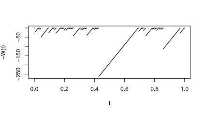
which is the trapping/waiting time of . In words: the event of the diffusion being trapped at a point at time until time happens precisely when . Hence the law of provides a weighting of the initial condition depending on the trapping/waiting time of . Notice that the process is self-similar with index and it is composed by right continuous degrees increasing slopes with leftmost limit (see Figure ).
6.1. A non-memory interpretation
It is possibly appealing to think about the values for the initial condition as the ‘depth’ underneath the surface where the particle moves. Then one can think about the particle as falling instantaneously at the bottom of a hole/trap of depth , and then taking time to climb back up to the surface. Then, at time one can observe the particle being -depth-units down in the hole. From this viewpoint, once the particle is in the hole it just drifts upward with unit speed. As a quick example, consider the variable separable initial condition where . Then the solution reads for
Hence, in this example the diffusive particle will have to be a least a unit deep in a hole (trapped for at least a unit time) for the values at its trapping point at its depth (in the past) to contribute to the solution.
A. Appendix
A.I. Continuity of solution (1.3) at
Proposition A.1.
For every , the following bound on small overshootings holds,
Proof. With the first equality holding by [29, Theorem 1 for ] along with the identity (2.3), compute
where and for every . Now pick . Then for every
hence for every
Then for every , which is equivalent to for every . And so we obtain
∎
We now use the bound in Proposition A.1 to prove the following continuity result
Proposition A.2.
Consider the function defined in (1.3), with an arbitrary -valued stochastic (sub-)process in place of , such that is stochastically continuous at . Also assume and is continuous at every point in . Then for every
Proof. Let . Let be arbitrary. Pick such that
Then
Now, by Proposition A.1, for all it holds that . Then the estimate above reads
To conclude, by stochastic continuity, pick a possibly smaller threshold to obtain
∎
Remark A.3.
The continuity at of Proposition A.2 is not obvious. For example it is clear that Proposition A.2 fails if we replace with a decreasing Poisson process. In fact Proposition A.2 fails in general if we replace with a decreasing compound Poisson process with generator
To see this, observe that for every
and note that the right hand side is non-decreasing as , where is the left continuous inverse of . As we can choose and so that
Now, consider a continuous non-negative with , such that . Then for every
A.II. Proof of Lemma 2.6-(i)-(ii)-(iii)
The three proofs are essentially the same, hence we prove only (ii).
Note that for every , and that
for every , . It is then easy to prove that is sub-Feller semigruop on . We denote the generator of by . Let , where and . Then, by a standard triangle inequality argument, we obtain
as . An induction argument proves that and on . Observing that is invariant under and it is a subspace of , if we can prove that is dense in , we are done by [15, Lemma 1.34]. So proceed by noting that set is a sub-algebra of that contains constant functions and separates points. Hence is dense in by Stone-Weierstrass Theorem for compact777In the case of unbounded domains (part (iii) of the current lemma) use the Stone-Weierstrass Theorem for locally compact Hausdorff spaces. Hausdorff spaces. We now prove density of the following set
For we take a sequence such that , where , for some depending on . Let and be smooth functions for each , such that , for and , and for and , where is compact, for each , and . Define for each ,
Then, as
As we need to work a bit more. For any we can now take a uniformly approximating sequence . Denote , for some depending on , where are non-zero, for each , . As and are dense in and , respectively, we can pick , in the following fashion: for each triplet , first pick so that
secondly pick so that
Then, after defining , we obtain
References
- [1] Allen, M.. Uniqueness for weak solutions of parabolic equations with a fractional time derivative. arXiv preprint arXiv:1705.03959 (2017).
- [2] Allen, M., Caffarelli L., Vasseur A.. A parabolic problem with a fractional time derivative. Archive for Rational Mechanics and Analysis 221.2 (2016): 603-630.
- [3] Baeumer, B., Kurita S., Meerschaert M. M.. Inhomogeneous fractional diffusion equations. Fractional Calculus and Applied Analysis 8.4 (2005): 371-386.
- [4] Baeumer, Boris, Tomasz Luks, and Mark M. Meerschaert. Space-time fractional Dirichlet problems. arXiv preprint arXiv:1604.06421 (2016).
- [5] Baeumer, Boris, and Mark M. Meerschaert. Stochastic solutions for fractional Cauchy problems. Fractional Calculus and Applied Analysis 4.4 (2001): 481-500.
- [6] Baeumer B, Meerschaert M, Nane E. Brownian subordinators and fractional Cauchy problems. Transactions of the American Mathematical Society. 2009;361(7):3915-30.
- [7] Barlow, Martin T.; C̆erný, Jir̆í. Convergence to fractional kinetics for random walks associated with unbounded conductances. Probability theory and related fields, 2011, 149.3-4: 639-673.
- [8] Benson DA, Meerschaert MM, Revielle J. Fractional calculus in hydrologic modeling: A numerical perspective. Advances in water resources. 2013 Jan 1;51:479-97.
- [9] Bernyk, Violetta, Robert C. Dalang, and Goran Peskir. Predicting the ultimate supremum of a stable Lévy process with no negative jumps. The Annals of Probability 39.6 (2011): 2385-2423.
- [10] J. Bertoin (1996) Lévy processes. Cambridge University Press.
- [11] Bingham, N. H. Limit theorems for occupation times of Markov processes. Zeitschrift für Wahrscheinlichkeitstheorie und verwandte Gebiete 17.1 (1971): 1-22.
- [12] Bobaru F , Duangpanya M . The peridynamic formulation for transient heat conduction. Int J Heat Mass Transf 2010;53(19):4047–59 .
- [13] Bonforte, M., Vázquez, J. L. (2016). Fractional nonlinear degenerate diffusion equations on bounded domains part I. Existence, uniqueness and upper bounds. Nonlinear Analysis, 131, 363-398.
- [14] Bogdan, K., Byczkowski, T., Kulczycki, T., Ryznar, M., Song, R., Vondracek, Z. (2009). Potential analysis of stable processes and its extensions. Springer Science & Business Media.
- [15] Böttcher, Björn, R. L. Schilling, and Jian Wang. Lévy matters. III.: Lévy-type Processes: Construction, Approximation and Sample Path Properties. Cham: Springer (2013).
- [16] Chen Z-Q, (2017). Time fractional equations and probabilistic representation, Chaos, Solitons & Fractals, 102, 168-174.
- [17] Chen, A., Du, Q., Li, C., Zhou, Z. (2017). Asymptotically compatible schemes for space-time nonlocal diffusion equations. Chaos, Solitons & Fractals, 102, 361-371.
- [18] Chen Zhen-Qing, Panki Kim, Takashi Kumagai, Jian Wang (2017). Heat kernel estimates for time fractional equations.arXiv:1708.05863.
- [19] Chen, Zhen-Qing, Mark M. Meerschaert, and Erkan Nane. Space-time fractional diffusion on bounded domains. Journal of Mathematical Analysis and Applications 393.2 (2012): 479-488.
- [20] Deng CS, Schilling RL. Exact Asymptotic Formulas for the Heat Kernels of Space and Time-Fractional Equations. arXiv preprint:1803.11435. 2018 Mar 30.
- [21] Diethelm, K. (2010), The Analysis of Fractional Differential Equations, An application-oriented exposition using differential operators of Caputo Type, Lecture Notes in Mathematics, v. 2004, Springer.
- [22] Du, Q., Yang, V., Zhou, Z., Analysis of a nonlocal-in-time parabolic equation. Discrete and continuous dynamical systems series B, Vol 22, n. 2, 2017.
- [23] Dynkin, E. B. (1965), Markov processes, Vol. I, Springer-Verlag.
- [24] Eidelman SD, Kochubei AN. Cauchy problem for fractional diffusion equations. Journal of differential equations. 2004 May 20;199(2):211-55.
- [25] Gilboa G , Osher S . Nonlocal operators with applications to image processing. Multiscale Model Simul 20 08;7(3):10 05–28 .
- [26] Du Q , Gunzburger M , Lehoucq RB , Zhou K . Analysis and approximation of nonlocal diffusion problems with volume constraints. SIAM Rev 2012;54(4):667–96 .
- [27] Fedotov S, Iomin A. Migration and proliferation dichotomy in tumor-cell invasion. Physical Review Letters. 2007 Mar 12;98(11):118101.
- [28] Hernández-Hernández, M.E., Kolokoltsov, V.N., Toniazzi, L., (2017). Generalised fractional evolution equations of Caputo type. Chaos, Solitons & Fractals, 102, 184-196.
- [29] Ikeda, Nobuyuki, and Shinzo Watanabe. On some relations between the harmonic measure and the Lévy measure for a certain class of Markov processes. Journal of Mathematics of Kyoto University 2.1 (1962): 79-95.
- [30] Krägeloh, Alexander M. Two families of functions related to the fractional powers of generators of strongly continuous contraction semigroups. Journal of mathematical analysis and applications 283.2 (2003): 459-467.
- [31] Leonenko NN, Meerschaert MM, Sikorskii A. Fractional pearson diffusions. Journal of mathematical analysis and applications. 2013 Jul 15;403(2):532-46.
- [32] M. Magdziarz: Path properties of subdiffusion–a martingale approach. Stoch. Models 26 (2010) 256–271.
- [33] Magdziarz M, Weron A, Weron K. Fractional Fokker-Planck dynamics: Stochastic representation and computer simulation. Physical Review E. 2007 Jan 26;75(1):016708.
- [34] M. Magdziarz, R.L. Schilling: Asymptotic properties of Brownian motion delayed by inverse subordinators. Proc. Amer. Math. Soc. 143 (2015) 4485–4501
- [35] Meerschaert, Mark M., David A. Benson, Hans-Peter Scheffler, Boris Baeumer. Stochastic solution of space-time fractional diffusion equations. Physical Review E 65, no. 4 (2002): 041103.
- [36] Meerschaert MM, Nane E, Vellaisamy P. Fractional Cauchy problems on bounded domains. The Annals of Probability. 2009;37(3):979-1007.
- [37] Meerschaert MM, Nane E, Vellaisamy P. Distributed-order fractional diffusions on bounded domains. Journal of Mathematical Analysis and Applications. 2011 Jul 1;379(1):216-28.
- [38] Meerschaert M.M., H.P. Scheffler: Limit theorems for continuous time random walks with infinite mean waiting times. J. Appl. Probab. 41 (2004) 623–638.
- [39] Meerschaert, M.M., Sikorskii, A. (2012), Stochastic Models for Fractional Calculus, De Gruyter Studies in Mathematics, Book 43.
- [40] Ming, Liao. The Dirichlet problem of a discontinuous Markov process. Acta Mathematica Sinica 5.1 (1989): 9-15.
- [41] Podlubny, I. (1998). Fractional differential equations: an introduction to fractional derivatives, fractional differential equations, to methods of their solution and some of their applications (Vol. 198). Elsevier.
- [42] Piryatinska A, Saichev AI, Woyczynski WA. Models of anomalous diffusion: the subdiffusive case. Physica A: Statistical Mechanics and its Applications. 2005 Apr 15;349(3-4):375-420.
- [43] Saichev AI, Zaslavsky GM. Fractional kinetic equations: solutions and applications. Chaos: An Interdisciplinary Journal of Nonlinear Science. 1997 Dec;7(4):753-64.
- [44] Samko, Stefan G., Anatoly A. Kilbas, and Oleg I. Marichev. Fractional integrals and derivatives. Theory and Applications, Gordon and Breach, Yverdon 1993 (1993): 44.
- [45] Scalas E, Five years of continuous-time random walks in econophysics, Complex Netw. Econ. Interactions 567 (2006) 3–16
- [46] Scalas E, R Gorenflo, F Mainardi. Fractional calculus and continuous-time finance. Physica A: Statistical Mechanics and its Applications, 2000.
- [47] Silling SA , Lehoucq RB . Peridynamic theory of solid mechanics. Adv Appl Mech 2010;44:73–168 .
- [48] Zaslavsky GM. Fractional kinetic equation for Hamiltonian chaos. Physica D: Nonlinear Phenomena. 1994 Sep 1;76(1-3):110-22.
- [49] Zhang Y, Meerschaert MM, Baeumer B. Particle tracking for time-fractional diffusion. Physical Review E. 2008 Sep 19;78(3):036705.
- [50] Zolotarev, V. M. (1986) One-dimensional stable distributions. Translations of Mathematical monographs, vol. 65, American Mathematical Society, 1986.