Tan’s contact scaling behaviour for trapped Lieb-Liniger bosons: from two to many

Abstract

We show that the contact parameter of $N$ harmonically-trapped interacting 1D bosons at zero temperature can be analytically and accurately obtained by a simple rescaling of the exact two-boson solution, and that $N$-body effects can be almost factorized. The small deviations observed between our analytical results and DMRG calculations are more pronounced when the interaction energy is maximal (i.e. at intermediate interaction strengths) but they remain bounded by the large-$N$ local-density approximation obtained from the Lieb-Liniger equation of state stemming from the Bethe Ansatz. The rescaled two-body solution is so close to the exact ones, that is possible, within a simple expression interpolating the rescaled two-boson result to the local-density, to obtain $N$-boson contact and ground state energy functions in very good agreement with DMRG calculations. Our results suggest a change of paradigm in the study of interacting quantum systems, giving to the contact parameter a more fundamental role than energy.

I Introduction

The relation between two-body and many-body physics is often an important point for the comprehension and the description of strongly-correlated quantum systems. A celebrated example is provided by homogeneous one-dimensional (1D) interacting systems solvable by the Bethe Ansatz, such as bosons and fermions with contact interactions LiebLin ; Yang67 ; Sutherland68 . In that case, the $N$-body solution can be exactly expressed as a function of a product of two-body scattering contributions. Generally, such a system is no longer integrable when subjected to an external potential but a notable exception is the limit of infinitely strong repulsive interactions, known as the Tonks-Girardeau limit, where fermionization occurs. In that case, the system remains exactly solvable, for any number of bosons and fermions Vignolo00 ; Deuretzbacher ; Fang2011 ; vignolo2013 ; Volosniev2014 ; Deuretzbacher2014 ; Decamp2016 ; Decamp2016b ; Decamp2017 . At finite interactions, the harmonically-trapped system can be exactly solved for 2 particles Busch98 and is approximately solved in the large-$N$ limit by a local density approximation (LDA) on the Lieb-Liniger solution Olshanii03 . For finite-$N$ systems, several approaches have been proposed: a pair-correlated wavefunction approach Brouzos2012 ; Koscik2018 ; a $T$-matrix approach for the Fermi polaron at zero and finite temperature Doggen2013 ; a geometric wavefunction description, that is very accurate for 2 and 3 bosons Wilson2014 ; and, more recently, an interpolatory Ansatz combining the non-interacting and unitary wavefunctions Andersen2016 . This last approach provides very accurate results for the energy in impurity systems Andersen2016 , but is less accurate when increasing the number of particle components Pecak2017 .

A crucial observable for a 1D system of $N$ particles with contact interactions is Tan’s contact parameter, characterizing the asymptotic behavior of the momentum distribution of the particles $C_{N}=\lim_{k\to\infty}k^{4}n(k)$ Minguzzi02 . The contact embeds information on the interaction energy and the density-density correlation function Tan2008a ; Tan2008b ; Tan2008c . It is a univocal measure of the wavefunction symmetry of fermionic and/or bosonic mixtures Decamp2016b ; Decamp2017 . The contact parameter is also determined by the probability density of finding 2 particles at a vanishing distance Olshanii03 . For trapped quantum gases, this probability density has a nontrivial dependence on the number of particles and on the interaction strength xu2015 ; Yao2018 .

In this Letter, we propose a change of paradigm by showing that the contact parameter plays in fact a more fundamental role than the energy in analyzing Lieb-Liniger bosons. Inspired by the scaling properties of this model, we show that if the starting point of the scaling analysis is the contact parameter instead of the energy, the two-body result provides a very good description of the system for any number of particles and interaction strengths. The quantitative difference between our predictions and numerically-exact DMRG results is always very small (i.e. less than a few percent) and is the largest at intermediate interaction strengths where the interaction energy is also the largest. For particle numbers $N>2$ we show that the many-body corrections to the rescaled two-body result can be accounted for by a simple interpolation connecting the two-body solution and the LDA one. With this, we obtain an analytical and very accurate expression for the contact parameter at all particle numbers $N$ that we use to derive an accurate formulation for the total energy of the system.

II Model and scaling analysis

We start with the case of $N\geq 2$ identical and harmonically-trapped 1D bosons of mass $m$ at zero temperature, interacting via repulsive contact interactions. Such a system is described by the many-body Hamiltonian

$$H=\sum_{j=1}^{N}\left[\frac{-\hbar^{2}}{2m}\frac{\partial^{2}}{\partial x_{j}^{2}}+\frac{1}{2}m\,\omega^{2}\,x_{j}^{2}+g\sum_{\ell>j}\delta(x_{j}-x_{\ell})\right]$$ (1)

with $g=2\hbar^{2}/(m|a_{\textrm{1D}}|)\geq 0$ Olsh98 . As shown by Tan in Tan2008a ; Tan2008b ; Tan2008c , the contact parameter associated to the eigenenergy $E_{N}$ reads

$$C_{N}(g)=\frac{m^{2}}{\pi\hbar^{4}}\left(-\frac{\partial E_{N}}{\partial g^{-1}}\right)=\frac{m^{2}g^{2}}{\pi\hbar^{4}}\frac{\partial E_{N}}{\partial g}\equiv\frac{m^{2}g}{\pi\hbar^{4}}E_{\textrm{int}}\,$$ (2)

where $E_{\textrm{int}}$ is the interaction energy. Tan’s contact Eq.(2) is thus a direct by-product of the dependence of the system energy on the interaction strength $g$. In the following, we will stick our analysis to the ground state energy. By rescaling Hamiltonian (1) by the ground state energy in the fermionized regime $E^{\infty}_{N}=N^{2}\hbar\omega/2$, and by expressing the particle coordinates in units of $a_{\textrm{ho}}/\sqrt{N}$, where $a_{\textrm{ho}}=\sqrt{\hbar/(m\omega)}$ is the harmonic oscillator length, it is easy to see that the ground state energy writes Decamp2016b

$$E_{N}(g)=E^{\infty}_{N}\,\mathcal{E}(N,g_{N})$$ (3)

where

$$g_{N}=\dfrac{mga_{\textrm{ho}}}{2\hbar^{2}\sqrt{N}}=\dfrac{a_{\textrm{ho}}}{|a_{\textrm{1D}}|\sqrt{N}}\equiv\dfrac{\alpha}{\sqrt{N}}$$ (4)

is the dimensionless interaction strength and $\alpha\!=\!a_{\textrm{ho}}/|a_{\textrm{1D}}|$. The dimensionless energy function $\mathcal{E}$ interpolates between the non-interacting regime where $\mathcal{E}(N,0)=1/N$ and the fermionized regime where $\mathcal{E}(N,\infty)=1$. Obviously, Tan’s contact depends on the same parameters $N$ and $g_{N}$ and reads:

$$C_{N}(g)=\dfrac{N^{5/2}}{\pi a_{\textrm{ho}}^{3}}\,\mathcal{C}(N,g_{N}),$$ (5)

where the rescaled dimensionless Tan’s contact

$$\mathcal{C}(N,z)=z^{2}\,\partial_{z}\mathcal{E}(N,z)$$ (6)

is evaluated at $z=g_{N}$. By the same token, $E_{\textrm{int}}=E^{\infty}_{N}\,\mathcal{E}_{\textrm{int}}(N,z)$ and we find

$$\mathcal{E}_{\textrm{int}}(N,z)=\dfrac{\mathcal{C}(N,z)}{z}=z\,\partial_{z}\mathcal{E}(N,z).$$ (7)

In the thermodynamic limit ($N,a_{\textrm{ho}}\to\infty$ at constant $a_{\textrm{ho}}/\sqrt{N}$), the only scaling parameter is $g_{N}$, both for the dimensionless energies $\mathcal{E}$, $\mathcal{E}_{\textrm{int}}$ and contact parameter $\mathcal{C}$. This can be easily shown in a Local Density Approximation (LDA) on the Lieb-Liniger homogeneous solution LiebLin ; Olshanii03 , and generalized to a generic trapping potential (see App. A). One gets:

$$\begin{split}&E^{\textrm{\tiny LDA}}_{N}(g)=E^{\infty}_{N}\,\mathcal{E}_{\textrm{\tiny LDA}}(g_{N})\\ &C^{\textrm{\tiny LDA}}_{N}(g)=\dfrac{N^{5/2}}{\pi a_{\textrm{ho}}^{3}}\,\mathcal{C}_{\textrm{\tiny LDA}}(g_{N})\end{split}$$ (8)

with $\mathcal{E}_{\textrm{\tiny LDA}}(0)\!=\!\mathcal{C}_{\textrm{\tiny LDA}}(0)\!=\!0$, $\mathcal{E}_{\textrm{\tiny LDA}}(\infty)\!=\!1$ and $\mathcal{C}_{\textrm{\tiny LDA}}(\infty)\!=\!128\sqrt{2}/(45\pi^{2})$ Olshanii03 . Although the derivation has been detailed for single-component bosons, it is possible to show that the scaling analysis applies also to multi-component bosons and fermions Massignan2015 ; Matveeva2016 ; Decamp2016b ; Lewenstein-Massignan ; Laird2017 , the Hamiltonian being the same as Eq. (1).

III The reduced contact parameter and scaling Ansatz

Strictly speaking, the LDA scaling behavior with respect to the sole variable $z$ should only hold in the large-$N$ limit. Indeed, it is what we observe if we plot $\mathcal{C}(N,z)$ obtained by a 2-tensor DMRG optimisation of a Matrix Product States (MPS) Ansatz  Schollwock2011 (see App. B) in comparison with $\mathcal{C}_{\rm LDA}(z)$, as shown in the left panel of Fig. 1.

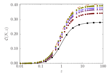
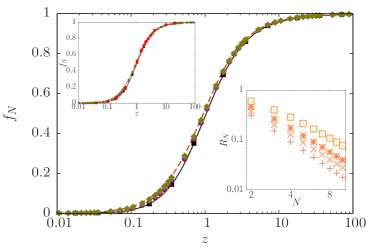
Figure 1: (Color online) Rescaled dimensionless contact $\mathcal{C}(N,z)$, Eq.(6), (left panel) and reduced contact parameter $f_{N}(z)$, Eq.(10), (right panel) as a function of the dimensionless scaling parameter $z=a_{\textrm{ho}}/(|a_{\textrm{1D}}|\sqrt{N})=a_{\textrm{ho}}/(|a_{\textrm{1D}}^{\prime}|\sqrt{2})$. The different symbols corresponds to DMRG calculations: $N=2$ (black squares), $N=3$ (brown circles), $N=4$ (purple triangles up), $N=5$ (light-blue triangles down) and $N=8$ (green diamonds). The black continuous line corresponds to Eq. (29), and the orange dashed line corresponds to the LDA solution, Eq. (8) Olshanii03 . Top inset in the right panel: Reduced contact parameter $f_{N}(z)$ for $SU(\kappa)$ fermions Decamp2016b (red points), $\kappa$ ranging from 2 to 6, superposed to all the data and curves of the main panel. Bottom inset in the right panel: Convergence rate $R_{N}(z)$ as a function of $N$, in a log-log scale, for $z=$ 0.14 (squares), 0.35 (stars), 0.70 (crosses), and $z\rightarrow\infty$ (plus).

However all the curves seem to have the same shape, but with different asymptotic values. Here we put forward a different scaling hypothesis by assuming that the reduced scaling parameter

$$f_{N}(z)=\dfrac{C_{N}(g(z))}{C_{N}(\infty)}=\dfrac{\mathcal{C}(N,z)}{\mathcal{C}(N,\infty)},$$ (9)

with $g(z)=2\hbar^{2}\sqrt{N}z/(ma_{\textrm{ho}})$, is an universal function for any $N\geq 2$. In particular, if this scaling hypothesis holds,

$$f_{N}(z)=f_{2}(z).$$ (10)

This would correspond to the assumption that a $N$-boson system at contact interaction strength $g$ is amenable to an effective 2-boson system at a rescaled weaker contact interaction strength $g^{\prime}=\sqrt{2/N}g$. Stated equivalently, the scattering length is renormalized through $a_{{\textrm{1}D}}\to a_{{\textrm{1}D}}^{\prime}=\sqrt{N/2}\,a_{{\textrm{1}D}}$. In the case of $N=2$ bosons, Tan’s contact is given by

$$C_{2}(g)=\dfrac{m^{2}g^{2}}{\pi\hbar^{4}}|\psi_{\nu}(0)|^{2}$$ (11)

where $\psi_{\nu}(0)$ is the wavefunction solving the Schrödinger equation for the relative motion Busch98 evaluated at $x_{1}-x_{2}=0$. It is straightforward (see App. C) to show that

$$f_{2}(z)=\dfrac{\mathcal{C}(2,z)}{\mathcal{C}(2,\infty)}=\dfrac{\pi\nu^{2}\,2^{\nu-1}}{\mathcal{N}(\nu)\,[\Gamma(1-\nu/2)]^{2}}$$ (12)

where $\mathcal{C}(2,\infty)=1/(2\sqrt{\pi})$, $\mathcal{N}(\nu)$ is a normalization factor (see App. C), and the $\nu$’s solve

$$\dfrac{\Gamma(-\nu/2)}{\Gamma(-\nu/2+1/2)}=-\dfrac{1}{z}.$$ (13)

In the right panel of Fig. 1, we compare the exact result for $f_{2}(z)$, Eq. (32), to the numerical data. The fact that all curves (almost) collapse show that $z=a_{\textrm{ho}}/(|a_{\textrm{1D}}|\sqrt{N})=a_{\textrm{ho}}/(|a_{\textrm{1D}}^{\prime}|\sqrt{2})$ is indeed the dimensionless scaling parameter of the reduced contact parameter, and that the contact for any interaction strength and any number $N$ of particles can be deduced from a simple 2-body calculation, $f_{2}(z)$, and from the knowledge of the contact for $N$ particles in the Tonks-Girardeau limit, $\mathcal{C}(N,\infty)$, that, for bosons, can be calculated exactly vignolo2013 . This means also that the function $C_{N}(\infty)$ almost embeds the full $N$-dependence of the problem for any value of $z$, even for few-body systems where the $N^{5/2}$ factor, deduced in the thermodynamic limit, starting from the energy scaling-analysis, fails. This result seems to be general and not to depend on the particle statistics Massignan2015 ; Matveeva2016 ; Decamp2016b ; Lewenstein-Massignan ; Laird2017 . Indeed, the data for the reduced contact parameter of a harmonically-trapped one-dimensional SU($\kappa$) interacting fermions Decamp2016b collapse on the same curve, as shown in the top inset in the right panel of Fig. 1.

III.1 Are two enough?

Our DMRG data match at first sight very well with the simple prediction of Eq. (10). However, we observe small deviations at intermediate interaction strengths where the data lie between $f_{2}$ (black continuous line) and the LDA solution $f_{\textrm{\tiny LDA}}=\mathcal{C}_{\textrm{\tiny LDA}}(z)/\mathcal{C}_{\textrm{\tiny LDA}}(\infty)$ (orange dashed line) that is known to be a very good approximation for the contact in the large-$N$ limit. This point is illustrated in the bottom inset of the right panel of Fig. 1, where we show, by plotting the convergence rate $R_{N}(z)=1-{\mathcal{C}(N,z)}/{\mathcal{C}_{\textrm{\tiny LDA}}(z)}$, how fast the exact contact converges to its LDA value at increasing $N$, for various values of $z$. A numerical fit in the fermionized regime vignolo2013 gives

$$R_{N}(\infty)=1-\dfrac{\mathcal{C}(N,\infty)}{\mathcal{C}_{\textrm{\tiny LDA}}(\infty)}\simeq 1.04\,N^{-7/4}.$$ (14)

The weak dependence on $z$ of the slope of the convergence rate $R_{N}(z)$ confirms that the dependence on $N$ of $C_{N}(z)$ is almost independent of $z$.

III.2 Beyond two

To further quantify the corrections to the scaling prediction Eq.(10), we plot in Fig. 2 the difference $\mathcal{D}_{N}(z)\!=\!f_{N}(z)\!-\!f_{2}(z)$.

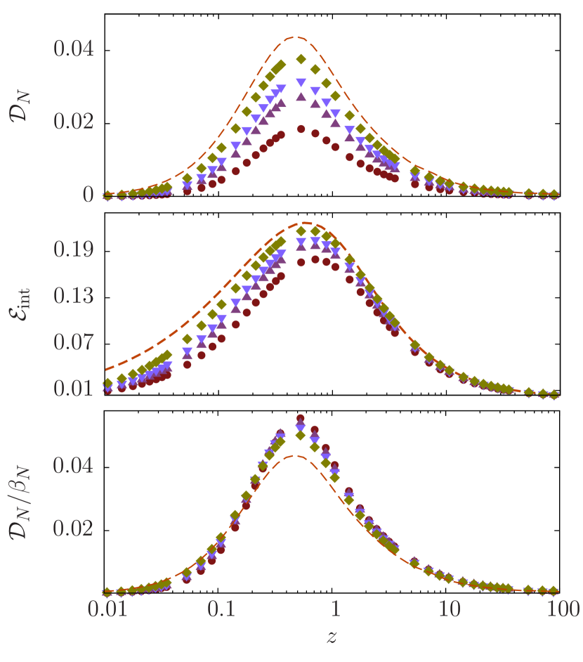
Figure 2: Top panel: (Color online) Difference $\mathcal{D}_{N}(z)\!=\!f_{N}(z)\!-\!f_{2}(z)$ for different values of $N$ as a funciton of the dimensionless scaling parameter $z$. Middle panel: Dimensionless interaction energy $\mathcal{E}_{\textrm{int}}(N,z)$ for different values of $N$, Eq.(7), as a function of $z$. All curves display a clear maximum at intermediate dimensionless interaction strengths $z\simeq 0.5$. Bottom panel: Scaled difference $\mathcal{D}_{N}(z)/\beta_{N}$ with $\beta_{N}=1-2/N$ for different values of $N$ as a function of $z$. All curves collapse quite well onto the LDA prediction $\mathcal{D}_{\textrm{\tiny LDA}}(z)$ (dashed orange curve) even if further corrections would be needed around the maximum. Symbols are the same as in Fig. 1.

We observe that $\mathcal{D}_{N}(z)$ reaches its largest value where the interaction energy $\mathcal{E}_{\textrm{int}}(N,z)$ is maximum. By comparing $\mathcal{D}_{N}(z)$ to the LDA prediction $\mathcal{D}_{\textrm{\tiny LDA}}(z)=f_{\textrm{\tiny LDA}}(z)-f_{2}(z)$ (orange dashed line), we infer the approximate, but quite accurate, proportionality relation $\mathcal{D}_{N}(z)\simeq\beta_{N}\,\mathcal{D}_{\textrm{\tiny LDA}}(z)$ with $\beta_{N}=1-2/N$, see bottom panel of Fig. 2. As a consequence, the simple interpolation

$$f_{N}(z)\simeq\left(1-\beta_{N}\right)\,f_{2}(z)+\beta_{N}\,f_{\textrm{\tiny LDA}}(z)$$ (15)

connects quite accurately the exact two-body solution for the contact parameter to the LDA one. We validate this interpolation in Fig. 3 by comparing Eq. (15) with DMRG data obtained for $N=3,4,5$ and $8$ bosons. We find a perfect agreement. This means that, within our approach, we can calculate with the same degree of precision all non-trivial experimentally relevant quantities that are directly connected to the contact parameter, such as the interaction energy Tan2008a ; Zwe11 , the two-body correlation function Olshanii03 ; Zwe11 , the magnetization Decamp2016b , the loss-rate in boson-fermion mixtures Sebastien2017 , or the heating rate due to measurement back-action of an atomic system in an optical cavity Uchino2018 .

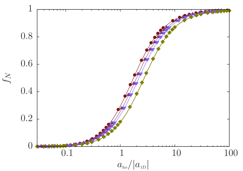
Figure 3: (Color online) Reduced contact parameter $f_{N}(\alpha/\sqrt{N})$, Eq.(10), for different $N$ and plotted as a function of $\alpha\!=\!a_{\textrm{ho}}/|a_{\textrm{1D}}|$ for better visibility. Solid lines: theoretical prediction Eq. (15); symbols: DMRG results. Symbols are the same as in Fig. 1.

IV From the contact to the energy

The most crucial test of the quality of our Ansatz for the contact parameter is the ground-state energy, since it is obtained by integration of the contact adding up the deviations:

$$\mathcal{E}(N,z)=1-\int_{z}^{\infty}dz^{\prime}\,\dfrac{\mathcal{C}(N,z^{\prime})}{z^{\prime 2}}.$$ (16)

Using Eq. (15), we arrive at

$$\begin{split}\mathcal{E}(N,z)&\simeq 1-\dfrac{2}{N}\,\dfrac{\mathcal{C}(N,\infty)}{\mathcal{C}(2,\infty)}\left[1-\mathcal{E}(2,z)\right]\\ &-\left(1-\dfrac{2}{N}\right)\,\dfrac{\mathcal{C}(N,\infty)}{\mathcal{C}_{\textrm{\tiny LDA}}(\infty)}\left[1-\mathcal{E}_{\textrm{\tiny LDA}}(z)\right].\end{split}$$ (17)

In Fig. 4, we plot the rescaled energy difference

$$\Delta_{N}(z)=\dfrac{E_{N}(g(z))-E_{N}(0)}{E_{N}^{\infty}-E_{N}(0)}=\dfrac{N\mathcal{E}(N,z)-1}{N-1},$$ (18)

whose limits $\Delta_{N}(\infty)\!=\!1$ and $\Delta_{N}(0)\!=\!0$ do not depend on $N$. We compare the exact numerical results with the prediction obtained by using Eq.(17) for different values of $N$ .

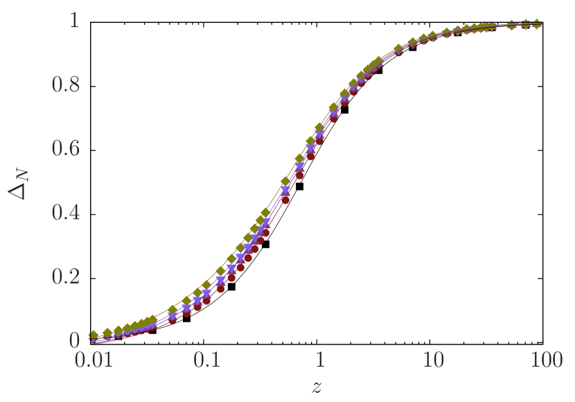
Figure 4: (Color online) Rescaled ground-state energy $\Delta_{N}(z)$ relative to its non-interacting value, Eq.(18), as a function of the dimensionless scaling parameter $z$ for different values of $N$. Solid lines: theoretical prediction Eq. (17); symbols: DMRG results, same $N$ values and symbols as in Fig. 1.

The agreement with the DMRG data is very good from moderately weak to strong interaction strengths ($z\geq 0.02$). Discrepancies only occur in the weak interaction regime ($z\leq 0.02$) where LDA is less accurate.

V Conclusion

We have shown that the contact parameter for $N$ harmonically-trapped interacting 1D bosons at zero temperature can be simply and accurately obtained from an appropriate rescaling of the two-body contact parameter followed by a smooth interpolation to the $N$-body LDA one. The key point is a change of paradigm: identifying the contact as the starting point for the scaling analysis instead of the energy. Indeed almost all the dependence of the contact on the number of particles can be embedded in the contact at infinite interactions for any number of particles. This result seems to be general and not to depend on the particle statistics. It shows the fundamental role of the contact, that is likely due to its local two-body correlation nature. We have further shown that our approach leads to a ground state energy for any number of bosons that matches very well the exact result down to moderately weak interaction strengths where no analytical solution is known. Our results improve on previous studies Brouzos2012 ; Wilson2014 ; Andersen2016 ; Pecak2017 with a simpler and more accurate Ansatz, that further confirm that the ground state properties of an interacting 1D Bose gas can be accurately described by an effective two-body contact interaction dressed by the other particles in the fluid Braaten2008 ; Zwe11 . Our work constitutes an important step forward in understanding the effects of correlations and interactions in harmonically-trapped one-dimensional interacting boson and fermion mixtures. It opens the way to further studies of similar scaling properties in higher-dimensional systems Levinsen2017 , confined in various trapping potentials, at zero and finite temperature Yao2018 .

Appendix A Scaling properties and Local Density Approximation for Tan’s contact parameter

We detail here the derivation of the scaling properties of $N$ one-dimensional bosons with contact interactions of strength $g$.

A.1 Scaling for the homogeneous system

For a homogeneous system of length $L$, the number density $\rho=L/N$ defines a length scale $\rho^{-1}$ and an energy scale $\hbar^{2}\rho^{2}/(2m)$. Scaling all spatial variables by $\rho^{-1}$ in the Hamiltonian Eq.(1) with $\omega=0$, it is easy to see that both the energy per particle and the energy density follow, in the thermodynamic limit, the scaling relations

$$\dfrac{E_{N}}{N}=\dfrac{\hbar^{2}\rho^{2}}{2m}\,e(\gamma),\qquad\dfrac{E_{N}}{L}=\dfrac{\hbar^{2}\rho^{3}}{2m}\,e(\gamma),$$ (19)

where $e(\gamma)$ is a monotonically increasing function of the dimensionless interaction strength

$$\gamma=\dfrac{mg}{2\hbar^{2}\rho}=\dfrac{1}{\rho|a_{\mathrm{1D}}|}=\dfrac{L}{N|a_{\mathrm{1D}}|}\equiv\dfrac{\alpha}{N}$$ (20)

where $\alpha=L/|a_{\mathrm{1D}}|$. The scaling relations Eq.(19) and the equation of state $e(\gamma)$ for the homogeneous system were exactly determined by Lieb and Liniger via the Bethe Ansatz LiebLin . In the thermodynamic limit $N,L\to\infty$ at constant density $\rho$, it takes values between $e(0)=0$ and $e(\infty)=\pi^{2}/3$. For $g\to\infty$, and for large $N$, we have $E^{\infty}_{N}\simeq N^{3}\epsilon_{0}/3$ where $\epsilon_{0}=\pi^{2}\hbar^{2}/(2mL^{2})$ is the ground-state energy of a particle in a box of size $L$. Then, from Tan’s relation for the contact parameter, see Eq.(2), it is easy to infer:

$$C_{N}(g)\simeq\dfrac{N\rho^{3}}{\pi}\,\gamma^{2}\dfrac{de}{d\gamma}=\dfrac{N^{4}}{\pi L^{3}}\,\gamma^{2}\dfrac{de}{d\gamma}$$ (21)

for the homogeneous system. Note that, following Eq.(3), we would have $\mathcal{E}(N,\gamma)\simeq 3e(\gamma)/\pi^{2}$ for the homogeneous system at large $N$.

A.2 Scaling for the harmonically-trapped system

In the presence of a harmonic potential, the appropriate thermodynamic limit is instead obtained by taking $N\to\infty$ and $\omega\to 0$ at constant $N\epsilon_{0}$ where $\epsilon_{0}=\hbar\omega/2$ is now the harmonic groundstate energy Decamp2016b . Stated equivalently, $N$ and $a_{\mathrm{ho}}\to\infty$ at constant ratio $\sqrt{N}/a_{\mathrm{ho}}$. Note that this ratio can be interpreted as an effective (constant) particle density $\rho=N/L_{N}$ in the thermodynamic limit for a system of size $L_{N}=\sqrt{N}a_{\mathrm{ho}}\to\infty$. Using this $\rho$ and $\hbar^{2}\rho^{2}/(2m)$ as the spatial and energy scales of the system, considerations analogous to the homogeneous case then lead to Eqs.(3-4) with $E^{\infty}_{N}=N^{2}\hbar\omega/2$, $\alpha=a_{\mathrm{ho}}/|a_{\mathrm{1D}}|$ and $\gamma=\alpha/\sqrt{N}$ $(\equiv g_{N})$. In particular, Eq.(21) immediately leads to Eq.(5-6) when replacing $\rho$ by $\sqrt{N}/a_{\mathrm{ho}}$.

Our approach is an alternative to the one developed in xu2015 where the scaling is expressed as a function of the parameter $\gamma(0)=mg/(\hbar^{2}\rho(0))$ where $\rho(0)$ is the density at the trap center.

A.3 Scaling for a general trapping potential

Let us considering the case of an arbitrary confining potential $V(x)$, in the case where the wavefunction vanishes at the boundaries. Denoting by $\epsilon_{n}=\eta_{n}\,\epsilon_{\xi}$ ($n\in\mathbbm{N}$) the consecutive energy levels of $V(x)$, where $\epsilon_{\xi}=\hbar^{2}/(2m\xi^{2})$ and $\xi$ are the characteristic energy and length scales of the trap, the thermodynamic limit is obtained in a similar way. Indeed, the ground state energy per particle in the infinitely-repulsive interacting limit then reads $E_{N}(g=\infty)/N=b(N)\,\epsilon_{\xi}$ where

$$b(N)=\dfrac{1}{N}\ \sum_{n=0}^{N-1}\eta_{n}\sim N^{2q}.$$ (22)

The thermodynamic limit is then obtained by taking $N\to\infty$ and $\xi\to\infty$ at constant ratio $N^{q}/\xi$. We would thus have $L_{N}=\xi\,N^{1-q}$ and $\gamma\equiv g_{N}=\alpha\,N^{-q}$. For the harmonic trap, one has $q=1/2$.

A.4 Local density approximation (LDA)

Such scaling forms for the harmonically-trapped system are recovered exactly in the LDA. We start from the chemical potential of the homogeneous system as obtained from the Lieb-Liniger equation of state:

$$\mu_{\mathrm{h}}=\dfrac{\partial E_{N}}{\partial N}=\frac{\hbar^{2}\rho^{2}}{2m}\,\left(3\,e(\gamma)-\gamma\frac{de}{d\gamma}\right).$$ (23)

By defining the interaction energy scale $\epsilon_{g}=\hbar^{2}/(2ma_{\mathrm{1D}}^{2})=4g/|a_{\mathrm{1D}}|$, we see that $\mu_{\mathrm{h}}=\epsilon_{g}\,F(\gamma)$ with:

$$F(\gamma)=3\dfrac{e(\gamma)}{\gamma^{2}}-\dfrac{1}{\gamma}\dfrac{de}{d\gamma}.$$ (24)

The above is a monotonous function of $\gamma$ for bosons in the Lieb-Liniger model LiebLin . Inverting this equation, we can obtain the particle density in terms of the chemical potential under the form $\rho|a_{\mathrm{1D}}|=n(\mu_{\mathrm{h}}/\epsilon_{g})$, where $n$ is a dimensionless function. In the presence of the harmonic potential $V_{\mathrm{ext}}(x)=m\omega^{2}x^{2}/2$, the inhomogeneous density profile within the LDA reads

$$\rho(x)=\frac{1}{|a_{\mathrm{1D}}|}\ n\left(\frac{\mu_{\mathrm{t}}-V_{\mathrm{ext}}(x)}{\epsilon_{g}}\right)\Theta(1-|x|/R),$$ (25)

where $\Theta$ is the Heaviside step function and $R=\sqrt{2\mu_{t}/(m\omega^{2})}$ the Thomas-Fermi radius.

The chemical potential of the trapped gas $\mu_{\mathrm{t}}$ is obtained by imposing the normalization condition $N=\int\rho(x)\mathrm{d}x$. After the change of variable $z=x/R$, and noting that $\epsilon_{g}=\hbar\omega\,\alpha^{2}/2$ and $R=a_{\mathrm{ho}}\,\sqrt{2\mu_{t}/(\hbar\omega)}$ it is easy to recast this normalization condition into

$$\sqrt{\dfrac{\mu_{t}}{\epsilon_{g}}}\,\int_{|z|\leq 1}n\left[\dfrac{\mu_{t}}{\epsilon_{g}}(1-z^{2})\right]\,\mathrm{d}z=\dfrac{1}{g^{2}_{N}}.$$ (26)

Just like for the homogeneous case, this equation can be inverted to give $\mu_{t}=\epsilon_{g}\,M(g_{N})$. By integrating backwards the chemical potential, $E_{N}(g)\equiv\int_{0}^{N}\mu_{\mathrm{t}}(N^{\prime})\,\mathrm{d}N^{\prime}$, the dimensionless LDA energy writes

$$\mathcal{E}_{\mathrm{LDA}}(g_{N})=\dfrac{2E_{N}(g)}{\hbar\omega N^{2}}=\dfrac{\alpha^{2}}{2}\,\int_{0}^{N}M\left(\alpha/\sqrt{N^{\prime}}\right)\,dN^{\prime}.$$ (27)

With the change of variables $y=\alpha/\sqrt{N^{\prime}}$, we finally arrive at

$$\mathcal{E}_{\mathrm{LDA}}(g_{N})=2g_{N}^{4}\,\int_{g_{N}}^{\infty}\dfrac{M(y)}{y^{3}}dy,$$ (28)

from which the LDA Tan’s contact parameter $\mathcal{C}_{\mathrm{LDA}}(z)=z^{2}\,\partial_{z}\mathcal{E}_{\mathrm{LDA}}(z)$ follows. For bosons in the Tonks-Girardeau regime, one has $\mathcal{C}_{\textrm{\tiny LDA}}(\infty)\!=\!128\sqrt{2}/(45\pi^{2})$ Olshanii03 . The corresponding expressions for multicomponent fermions in the limit of infinite repulsive interactions have been derived in Decamp2016b .

Appendix B Density Matrix Renormalization Group (DMRG)

The numerical results for the Tan’s contact of several particles at finite interactions have been obtained by a two-tensor DMRG optimisation of a Matrix Product States (MPS) Ansatz Schollwock2011 . Namely, we take a (tight-binding) lattice discretization of Eq.(1) in a sufficiently large box ($L$ up to 12 $a_{\mathrm{ho}}$), and we extract the continuum limit by considering lattice spacings $a$ down to $a_{\mathrm{ho}}/16$: the tunneling amplitude, external potential and on-site interaction strength scale like $t\propto a^{-2}$, $V\propto a^{2}$, and $U\propto a^{-1}$ respectively. We encompass the conservation laws of the particle number in the tensor network structure directly, in order to achieve both speed-up and increased accuracy. The discarded probability is kept below $10^{-12}$, and no truncation is performed on the local bosonic Hilbert space. For more details, we refer the reader, e.g., to a recent work of ours Decamp2016b .

Appendix C Reduced contact parameter for 2 bosons

In the case of $N=2$ bosons, Tan’s contact is given by

$$C_{2}(g)=\dfrac{m^{2}g^{2}}{\pi\hbar^{4}}|\psi_{\nu}(0)|^{2}$$ (29)

where

$$\psi_{\nu}(0)=\dfrac{(\pi/2)^{1/4}}{\sqrt{a_{\textrm{ho}}}\sqrt{\mathcal{N}(\nu)}}\dfrac{2^{\nu/2}}{\Gamma(-\nu/2+1/2)}\,\Phi\left(-\dfrac{\nu}{2},\dfrac{1}{2},0\right)$$ (30)

is the wavefunction solving the Schrödinger equation for the relative motion Busch98 evaluated at $x_{1}-x_{2}=0$. $\Gamma(u)$ is the gamma Euler function, $\Phi$ is the (Kummer) hypergeometric function, and

$$\mathcal{N}(\nu)=\Gamma(\nu+1)\left\{1+\tfrac{\sin(\pi\nu)}{2\pi}\left[\mathtt{\Psi}\left(\tfrac{\nu}{2}+1\right)-\mathtt{\Psi}\left(\tfrac{\nu}{2}+\tfrac{1}{2}\right)\right]\right\}$$ (31)

is a normalization factor involving the digamma function $\mathtt{\Psi}(u)=\Gamma^{\prime}(u)/\Gamma(u)$. It is straightforward to show that

$$\dfrac{\mathcal{C}(2,g_{2})}{\mathcal{C}(2,\infty)}=\dfrac{\pi\nu^{2}\,2^{\nu-1}}{\mathcal{N}(\nu)\,[\Gamma(1-\nu/2)]^{2}}\equiv f_{2}(g_{2})\,$$ (32)

where $\mathcal{C}(2,\infty)=1/(2\sqrt{\pi})$. The $\nu$’s are indeed a function of $\alpha/\sqrt{2}$ since they solve

$$\dfrac{\Gamma(-\nu/2)}{\Gamma(-\nu/2+1/2)}=\dfrac{\sqrt{2}}{\alpha}=\dfrac{1}{g_{2}}$$ (33)

and are the analog of the integers labeling the Hermite polynomials in the harmonic oscillator Busch98 . Noticeably, for $\nu\,\in\,[0,1]$, we have $\mathcal{N}(\nu)\simeq 1$, $[\Gamma(1-\nu/2)]^{-2}\simeq[1-(1-1/\pi)\nu]$ and

$$f_{2}(g_{2})\simeq\nu^{2}\,2^{\nu-1}\,[\pi-(\pi-1)\nu].$$ (34)

References

- (1) E. Lieb and W. Liniger, Phys. Rev. 130, 1605 (1963).
- (2) C. N. Yang, Phys. Rev. Lett. 19, 1312 (1967).
- (3) B. Sutherland, Phys. Rev. Lett. 20, 98 (1968).
- (4) P. Vignolo, A. Minguzzi, and M. Tosi, Phys. Rev. Lett. 85, 2850 (2000).
- (5) F. Deuretzbacher et al., Phys. Rev. Lett. 100, 160405 (2008).
- (6) B. Fang et al., Phys. Rev. A 84, 023626 (2011).
- (7) P. Vignolo and A. Minguzzi, Phys. Rev. Lett. 110, 020403 (2013).
- (8) A. Volosniev et al., Nature Communications 5, 5300 (2014).
- (9) F. Deuretzbacher et al., Phys. Rev. A 90, 013611 (2014).
- (10) J. Decamp et al., New Journal of Physics 18, 055011 (2016).
- (11) J. Decamp et al., Physical Review A 94, 053614 (2016).
- (12) J. Decamp et al., New Journal of Physics 19, 125001 (2017).
- (13) T. Busch, B.-G. Englert, K. Rza̧żewski, and M. Wilkens, Found. Phys. 28, 549 (1998).
- (14) M. Olshanii and V. Dunjko, Phys. Rev. Lett. 91, 090401 (2003).
- (15) I. Brouzos and P. Schmelcher, Phys. Rev. Lett. 108, 045301 (2012).
- (16) P. Kościk, M. Plodzień, and T. Sowiński, arXiv:1804.06342 (2018).
- (17) E. V. H. Doggen and J. J. Kinnunen, Phys. Rev. Lett. 111, 025302 (2013).
- (18) B. Wilson et al., Phys. Lett. A 378, 1065 (2014).
- (19) M. E. S. Andersen et al., Scientific Reports 6, 28362 (2016).
- (20) D. Pȩcak, A. S. Dehkharghani, N. T. Zinner, and T. Sowiński, Phys. Rev. A 95, 053632 (2017).
- (21) A. Minguzzi, P. Vignolo, and M. Tosi, Phys. Lett. A 294, 222 (2002).
- (22) S. Tan, Ann. Phys. (N.Y.) 323, 2971 (2008).
- (23) S. Tan, Ann. Phys. (N.Y.) 323, 2987 (2008).
- (24) S. Tan, Ann. Phys. (N.Y.) 323, 2952 (2008).
- (25) W. Xu and M. Rigol, Phys. Rev. A 92, 063623 (2015).
- (26) H. Yao et al., arXiv:1804.04902 (2018).
- (27) M. Olshanii, Phys. Rev. Lett. 81, 938 (1998).
- (28) P. Massignan, J. Levinsen, and M. M. Parish, Phys. Rev. Lett. 115, 247202 (2015).
- (29) N. Matveeva and G. Astrakharchik, New Journal of Physics 18, 065009 (2016).
- (30) T. Grining et al., Phys. Rev. A 92, 061601 (2015).
- (31) E. K. Laird, Z.-Y. Shi, M. M. Parish, and J. Levinsen, Phys. Rev. A 96, 032701 (2017).
- (32) U. Schollwöck, Ann. Phys. 326, 96 (2011).
- (33) M. Barth and W. Zwerger, Ann. Phys. 326, 2544 (2011).
- (34) S. Laurent et al., Phys. Rev. Lett. 118, 103403 (2017).
- (35) S. Uchino, M. Ueda, and J.-P. Brantut, arXiv:1802.04024 (2018).
- (36) E. Braaten and L. Platter, Phys. Rev. Lett. 100, 205301 (2008).
- (37) J. Levinsen, P. Massignan, S. Endo, and M. M. Parish, Jour. of Phys. B 50, 072001 (2017).