The Spatial—Kinematic Structure of the Region of Massive Star Formation S255N on Various Scales

ASTRONOMY REPORTS Vol. 62 No. 5 2018

Abstract

The results of a detailed analysis of SMA, VLA, and IRAM observations of the region of massive star formation S255N in CO(2—1), N₂H⁺ (3—2), NH₃ (1,1), C¹⁸O (2—1)and some other lines is presented. Combining interferometer and single-dish data has enabled a more detailed investigation of the gas kinematics in the moleclar core on various spatial scales. There are no signs of rotation or isotropic compression on the scale of the region as whole. The largest fragments of gas ($\approx$0.3 pc) are located near the boundary of the regions of ionized hydrogen S255 and S257. Some smaller-scale fragments are associated with protostellar clumps. The kinetic temperatures of these fragments lie in the range 10— 80 K. A circumstellar torus with inner radius R_in $\approx$ 8000 AU and outer radius R_out 12 000 AU has been detected around the clump SMA1. The rotation profile indicates the existence of a central object with mass $\approx$ 8.5/ sin 2 (i) M_⊙ . SMA1 is resolved into two clumps, SMA1—NE and SMA1—SE, whose temperatures are $\approx$150 K and $\approx$25 K, respectively. To all appearances, the torus is involved in the accretion of surrounding gas onto the two protostellar clumps.

1 Introduction

Studies of molecular clouds have attracted considerable attention. Much effort has gone into both simulations and observations of these objects (see, e.g., (Mapelli, 2017; Sokolov et al., 2017)). However, there remain relatively few well studied regions of high-mass star formation. They are encountered more rarely than the regions of low-mass star formation, and are located at large distances from the Sun, complicating observations of them. In relation to detailed studies of processes occurring in their cores, the resolution of single dishes is insufficient, while interferometers have limited sensitivity to extended structures.

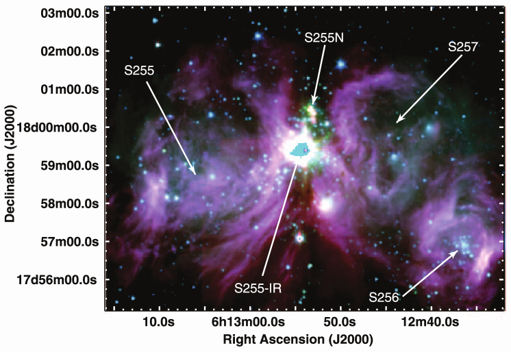
Figure 1: Spitzer IRAC three-color image of the region S255N and its surroundings, composed of images at 8.0 $\mu$m (red), 4.5 $\mu$m (green), and 3.6 $\mu$m (blue). S255N is located in a complex of regions of current and past star formation (Cyganowski et al., 2007). The color figures here and below are accessible in the electronic version of the journal.

The object considered in the current study is part of a molecular cloud (Richardson et al., 1985; Pirogov et al., 2003) located between the two zones of ionized hydrogen S255 and S257 (Fig. 1). It is supposed that the entire S254—S258 complex was formed by successive star formation(Bieging et al., 2007): expansion ofthe HII zones led to the compression of gas in the molecular cloud. This cloud contains three cores: S255IR, S255S, and S255N. The first is located in a later stage of evolution (Wang et al., 2011; Ojha et al., 2011): its radiation is appreciably brighter in the IR, and water-vapor and Class II methanol maser emission is detected in this region (Zinchenko et al., 2012; Kurtz et al., 2004). The core S255S is the youngest of the three, as is testified to by its lower brightness in the IR and in the 1.3 mm lines, as well as the compactness of the outflow in the core (Wang et al., 2011). A smaller number of 1.3 mm molecular lines is detected [6], and there are no signs of massive-star formation; we accordingly did not consider it in the current study.

The molecular cloud with which S255N (Sh2-255 FIR1, G192.60-MM1) is associated has been observed on several single-dish radio telescopes (OSO 20 m, IRAM 30 m, NRAO 12 m) (Zinchenko et al., 2009); the core of S255N has been observed with the SMA and VLA interferometers (Zinchenko et al., 2012). We present here combined data for the first time. The mass of the S255N core indicated by single-dish observations is $\sim$300 M_⊙, with n${}_{H_{2}}$ $\sim$2$\times$10⁵ cm^-3, T_k $\sim$40K, $\Delta$V $\sim$2km/s. The luminosity of the core is of order 10⁵ L_⊙ (Minier et al., 2007). An ultracompact HII region is observed in this region(Kurtz et al., 1994), as well as H₂O and Class I CH₃OH masers. These characteristics of the core provide evidence for the formation of massive stars in this region. A lack of coincidence in the positions of the emission peaks in the CO(2—1), HCN(1—0), HNC(1—0), HCO⁺(1—0), C¹⁸O (2—1), and C³⁴S(5—4) molecular lines has also been demonstrated (Zinchenko et al., 2009). The presence of hot, massive protostellar clumps in the core was shown in (Zinchenko et al., 2012; Cyganowski et al., 2007), with the velocity of half of the cores are different from the velocity of the ambient gas. The mass of the brightest of these clumps is $\approx$16 M_⊙ (Zinchenko et al., 2012) for a distance of 1.78 kpc(Burns et al., 2016). The presence of two spectral components in the (1, 1) ammonia lines in directions not coincident with a hot clump was detected in(Zinchenko et al., 2012). Several high-velocity outflows are present in the core, which also indicates rich gas kinematics. We attempted in the current study to estimate the motion of gas on scales fom the size of the core to the sizes of clumps, based on the collected data. We also used non-standard data-analysis methods that are robust to a noise to analyze emission that is weak against the background of the hot-clump emission. We used original methods to detect and identify kinematic fragments of the core, which were traced in position–velocity diagrams in a number of molecular lines.

2 Observational data and analysis

We considered data obtained on the SMA(Wang et al., 2011; Zinchenko et al., 2012) and VLA(Zinchenko et al., 2012) interferometric arrays and the 30-m IRAM telescope (Wang et al., 2011; Zinchenko et al., 2012). Table 1 presents a list of the observed molecules, the frequencies of their transitions, and the instruments used. All the data were reduced anew, and self-calibration was appied to the data of (Zinchenko et al., 2012). The CO(2—1), C¹⁸O (2—1), CH₃CN(12—11), and SO(6₅—5₄) lines were observed twice in the compact and once in the extended configuration of the SMA. These data were inverted into a single image at each line. The width of the synthesized antenna beam was $\approx$ 1.14^′′ at 217 GHz and $\approx$ 3.4^′′ for the remaining observations (the compact configuration of the SMA). The width of the VLA beam was $\approx$ 2.55^′′ (23.7 GHz), and the width of the IRAM beam was 12^′′ (217 GHz). The coordinates of the phase center for the SMA observations were $\alpha$(2000)=06^h12^m53.800^s, $\delta$(2000)=17^∘59^′22.097^′′.

2.1 Data reduction

Since one of the main aims of our study was to investigate the kinematics of the protostellar core on various spatial scales, we considered objects detected earlier in the 255N core with various extents from 2.5$\times$10^-3 pc to 0.48 pc [11]. The maximum angular sizes to which the instruments used at the various frequencies are sensitive are 66^′′ for the VLA and 25^′′ for the SMA, which corresponds to linear sizes of 0.52 and 0.2 pc at a distance of 1.78 kpc (Minier et al., 2007). These limits hinder the interpretation of observations over a wide range of spatial scales. An important role is also played by the loss of flux by the interferometer, which we compensated for by combining the interferometric and single-dish data. As an example, the profile of the CO(2—1) line indicated by the SMA observations differs strongly from the profile observed on the IRAM 30-m telescope in the same direction. Therefore, we consolidated the SMA data with the observations on the 30-m IRAM antenna. This was carried out for the N₂H⁺ (3—2), CO(2—1), and SiO(5—4) lines, as well as the 1.3-mm continuum observations. The spectral-line data were combined in the visibility domain based on the relative integrated-flux calibration in the region of overlapping spatial frequencies; the reconstructed continuum images were consolidated via a Fourier transform using standard procedures of the MIRIAD package (Sault et al., 1995). The “wings” of the CO(2—1) line at 3–7 km/s and 11–15 km/s from the single-dish data were used for the relative flux calibration of the synthesized visibilities at the frequency of this line.

CO(2—1), C¹⁸O(2—1), SO(6₅—5₄), DCO⁺(4—3), DCN(3—2) data were self-calibrated using the observations in the CH₃OH ($4_{2}$-$3_{1}$) line (Zinchenko et al., 2012). The self-calibration based on this line was fairly effective, since a single maser source was observed in the telescope field (Schwab, 1984).

2.2 Identification of kinematic fragments of the core

The presence of at last two spectral components with different Doppler velocities in the 255N region was noted earlier (Zinchenko et al., 2012), however their spatial distribution was not studied. In our current study, we carried out a careful analysis of the data considered, with the aim of conducting a detailed study of the spatial—kinematic structure of the core.

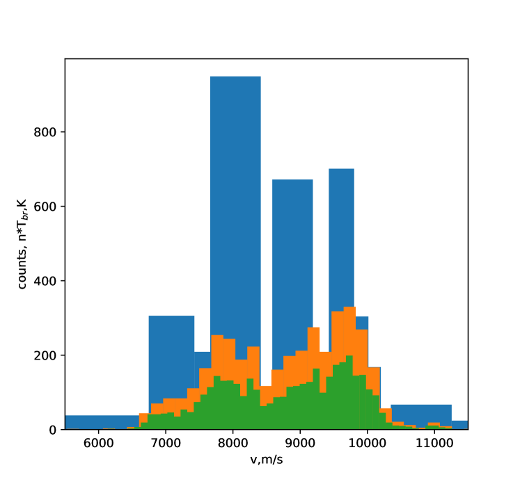
Figure 2: Example of the velocity distribution of the NH₃ (1,1)intensities derived using various algorithms for choosing the bin width. The blue columns show the results for the Bayesian block method, the orange bins the results of applying the Knuth rule, and the green columns results for a bin width of 0.2 km/s.

Application of the moment method for the identification of kinematic fragments does not always provide the best solution, especially for lines of molecules with hyperfine structure, such as NH₃ and N²H⁺, since such estimates can be shifted due to asymmetry of the line caused by its hyperfine structure. In addition, in the case of observations of two or more spectral components, the first moment yields an estimate of their mean velocity. Determining the spatial boundaries of components precisely is problematic, since they can interact, overlap, and be represented differently in different molecular lines, depending on whether or not the conditions in the components are the same. Therefore, we estimated the minimum number of boundaries from the number of peaks in a histogram of the line intensities as a function of their velocities (Fig. 2). Thus, instead of a spatial distribution, we obtained the distribution of the line intensities in various velocity ranges. This characterizes the distribution of the density, temperature, or some other physical parameter, depending on what quantity is traced by the studied line. We chose three molecular lines for this analysis: CO(2—1), N₂H⁺ (3—2), and NH₃ (1,1). We expected to observe signs of fragments in the outer, rarified layers of the core in the CO line. The emission in NH₃ and N²H⁺ is excited in quiescent and dense regions of the core. It is possible to obtain more accurate velocity estimates using these lines, since their transitions display hyperfine structure. Their spectra are fitted fairly well with the local thermodynamic equilibrium (LTE) model presented below. The shape of the histogram (Fig. 2) provides information about the internal structure of the core – whether it is homogeneous or is appreciably perturbed, and also whether the gas can be described as forming isolated or overlapping velocity components (that is, as kinematic fragments of the core), or whether the gas is involved in some process with a single spectral distribution.

We estimated the positions of the line centers by fitting model line profiles for the transition to the observed spectra, taking into account hyperfine structure in an LTE approximation with a Gaussian optical-depth profile:

$$T(\nu)=\sum_{n_{g}=1}^{m}(J(T_{ex}^{n_{g}})-J(T_{bg}))(1-e^{-\tau_{n_{g}}(v)}),$$ (1)

$$\tau_{n_{g}}(v)=\sum_{i=1}^{n_{hfs}}16\pi^{3}\nu_{ref}^{4}\mu^{2}\frac{Sg_{i}N_{u}^{n_{g}}}{3c^{3}J(T_{ex}^{n_{g}})}\phi_{n_{g}i}(v),$$ (2)

$$\phi_{n_{g}i}(v)=\frac{1}{\sqrt{2\pi}\sigma_{n_{g}}}e^{\frac{-(v-v_{i}-v_{n_{g}})^{2}}{2\sigma_{n_{g}}^{2}}},$$ (3)

where $T_{ex}^{n_{g}}$ is the excitation temperature of spectral component $n_{g}$, $N_{u}^{n_{g}}$ the column density of the molecules in the upper level for the transition considered, $\sigma_{n_{g}}$ the line width, $v_{n_{g}}$ the position of the line-component center (the subscript $n_{g}$ denotes the desired parameters of the model used in the fitting), $J(T)=\frac{h\nu/k}{exp(h\nu/kT)-1}$, $T_{bg}=2.73K$ is the cosmic microwave background temperature, $\nu_{ref}$ the transition frequency, $\mu$ the dipole moment, $S$ the line strength, $g_{i}$ the statistical weight of transition i of the hyperfine structure, $n_{hfs}$ the number of components of the hyperfine structure (18 for NH₃(1,1), 24 for NH₃(2,2), 38 for N₂H⁺(3—2)) $v_{i}$ the Doppler velocity of the transition $i$ in the line, and $m$ the number of spectral components in the line.

The values of $S$,$g_{i}$ and$v_{i}$ were taken from the CDMS database (Müller et al., 2005). The approximation was applicable for the NH₃ (1,1) and (2,2) and N₂H⁺(3—2) lines. At a number of positions on the map, two peaks were observed in the spectrum; accordingly, we allowed for the possibility of fitting lines containing $m$ independent spectral components. In our data sets, $m$ did not exceed two. The choice between one or two components was based on a comparison of the rms deviations in the spectrum after subtracting the model. If the ratio of the deviations for $m$=2 and $m$=1 was less than 1.4, we used the two-component model.

Thus, after fitting a line at each point in the map, we had estimates of the Doppler shifts of one or two spectral components. However, the number of kinematic components over the entire map can be appreciably greater than two. The number of such components can be estimated from a histogram of the velocity distribution of the line intensities. In the simplest case, the integrated intensities of the spectral components whose Doppler velocities lay within a given bin of the histogram were added. There also exist a large number of methods enabling choice of the bin width based on the data set considered, two of which we used in our analysis: the rule of Knuth (Knuth, 2006) and the Bayesian block method (Scargle et al., 2013), as realized in the astropy library (Astropy Collaboration et al., 2013). Figure 2 presents examples of applying these various methods.

Since a large fraction of a map contains lines with intensities at the detection threshold (3—5$\sigma$), and the channel width is of order the line width (5 in a group, 25 in a line, in the case of ammonia), we estimated the velocity using the k nearest neighbors (kNN) method (Altman, 1992), since least-squares fitting for these regions either diverged or converged to a local minimum, with the suppression of one component by the other. Based on the fitting at each point in the map, regions were chosen whose $\chi^{2}$ values for the LTE approximation were less than unity. The spectra at these points were used as a reference set of objects relative to which the remaining regions were considered. The velocities were estimated as

$$v_{k}=\frac{\sum_{i=1}^{n}v_{i},d(s_{k},s_{i})^{2}}{\sum_{i=1}^{n}d(s_{k},s_{i})^{2}}$$ (4)

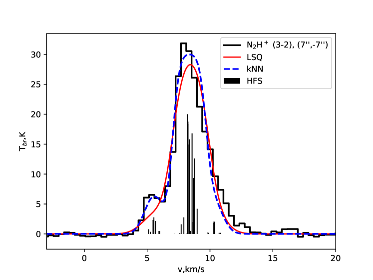
Figure 3: Observed N₂H⁺ (3—2)spectrum at the point (-7^′′ , 7^′′) relative to S225N–SMA1 (histogram), together with fits obtained using the least squares method (red solid curve) and the kNN method (blue dashed curve). The vertical lines with lengths proportional to their statistical weights denote hyperfine components of the (3—2) transition.

where $v_{k}$ is the velocity in a spectrum of interest, $v_{i}$ the velocity for the known (reference) spectrum, $s_{k}$, $s_{i}$ a spectrum of interest and a spectrum whose estimated velocity is known, $n=5$ the number of nearby spectra used to estimate the velocity, $d(s_{1},s_{2})=\sqrt{\sum_{j=1}^{m}(s_{1_{j}}-s_{2_{j}})^{2}}$ the distance in intensity space between the two spectra (analogous to the least-squares residual), $m$ the number of channels, and $s_{i_{j}}$ the intensity of the spectrum in channel $j$. In this form, the method resembles least squares fitting, but the algorithm for the descent of the parameters to those yielding the minimum residual is replaced by a search of n ”similar” spectra from the reference set. Examples of fitting a spectrum using the least-squares method and the first nearest neighbor method are presented in Fig. 3. The $\chi^{2}$ value for the LTE approximation is 266 (Jy/beam)² , and for the first nearest neighbor method is 72 (Jy/beam) ². A more detailed analysis of the k nearest neighbors method will be described in future publications.

2.3 Analysis of methanol observations

Estimates of the physical parameters (kinetic temperature and density of molecular hydrogen, specific column density (column density of molecules per unit velocity interval), and relative methanol abundance) were carried out using the database of methanol energy-level populations (Salii, 2006). This database contains methanol energy-level populations calculated at nodes of a parameter grid. The parameter values were varied from those corresponding to a dark molecular cloud to values that may be realized in regions heated by an embedded object or excited by the passage of a shock. The kinetic temperature was varied from 10 to 220 K, the density of molecular hydrogen from $10^{3}$ to $10^{9}$ cm^-3, the abundance of methanol relative to hydrogen from $10^{-9}$ to $10^{-6}$, and the specific methanol column density from $10^{8}$ to $10^{13}$ cm^-3s. The computations of the methanol level populations in the database were carried out in the LVG approximation. A model for the excitation of the methanol molecule developed for the conditions characteristic for star-forming regions, including regions of massive-star formation, was used in the computations (Cragg et al., 2005).

3 Results

3.1 Spatial–kinematic structure of the core

To investigate the kinematics of the gas inside the core, we considered first and foremost the emission in the N₂H⁺ (3—2)and NH₃ (1,1)lines, since these trace dense, quiescent gas. In addition, both lines contain hyperfine structure, making it possible to accurately measure Doppler shifts, and thereby the velocity of the gas. We compared the N₂H⁺ (3—2)data with the data for the CO(2—1), (6₅—5₄), and C¹⁸O (2—1)lines in a position–velocity diagram (see Fig. 9).

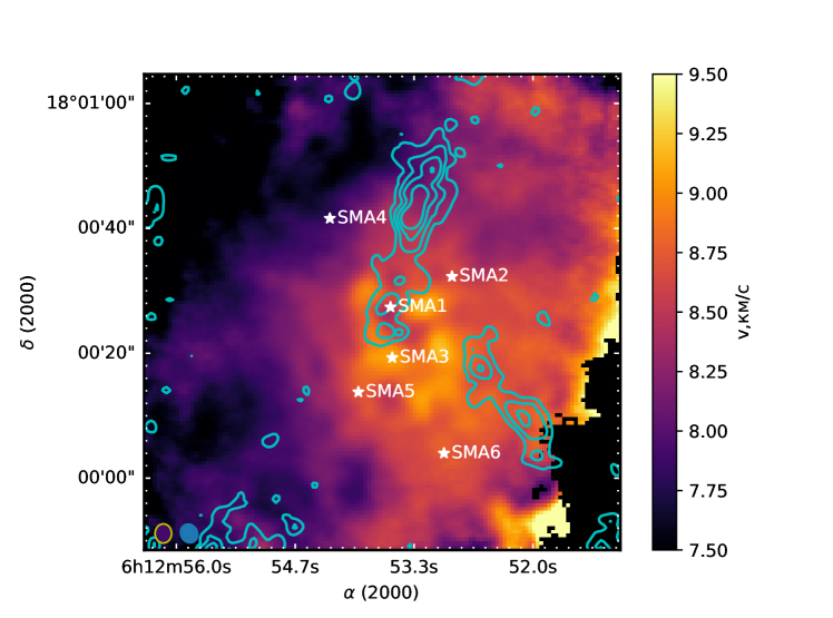
Figure 4: Map of the first moment of the CO(2—1) line (background). Contours of the (1, 1) ammonia intensity at levels of [4, 5.4, 6.8, 8, 9.5] K are superposed. The stars show the positions of clumps according to the data of (Zinchenko et al., 2012).

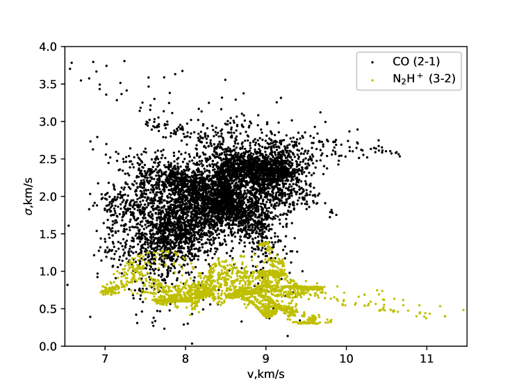
Figure 5: Dependence of the second moment (width) on the first moment (velocity) of the CO (2—1) and N₂H⁺ (3—2)lines.

The S255N core is part of a more extended structure (Richardson et al., 1985), which is also observed in our data. The CO(2—1) line emission has no boundary at the north and south of the map, as can be seen in Fig. 4 (combined data). The map of the first moment of this line on scales exceeding 20^′′ corresponds to the map presented in (Pirogov et al., 2003). However, a comparison of the first and second moments of the CO line (Fig. 5) indicates that the line width grows toward the center of the velocity range in a close to linear shape. The direction of the velocity variations is close to the direction toward the ionized regions S255 and S257 from the center of the map, with the mean gas velocity observed at the map center. There is no clearly distinguished symmetry axis, such as would be characteristic for the presence of rotation, as was shown in (Mapelli, 2017). Such a distribution would not be characteristic for an isotropic collapse. However, the broadening of lines toward the center of the velocity range may indicate mixing of two portions of gas driven by the expansion of envelopes.

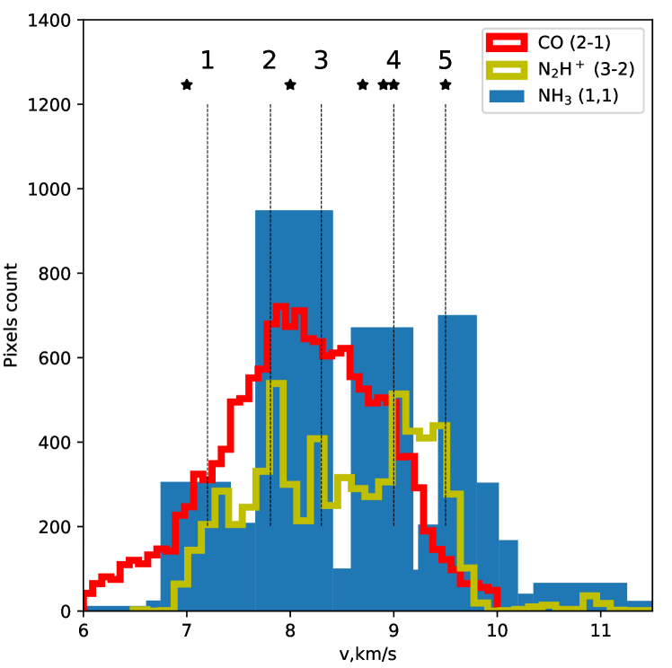
Figure 6: Histograms of the velocity distributions in various lines. The numbers and vertical dotted lines denote bands corresponding to the positions of kinematic fragments of the core. Maps of the first moment were used to construct the CO velocity histogram, and velocity estimates obtained with the kNN method were used for the remaining lines. The stars denote the velocities of clumps according to the data of (Zinchenko et al., 2012).

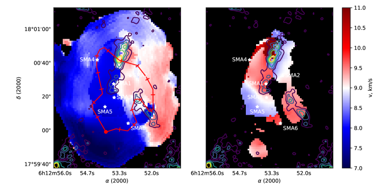
Figure 8: Maps of the Doppler velocity of the spectral components of the N₂H⁺ (3—2)line derived from the combined SMA and IRAM data. The left and right images show the velocities of the blue and red components in the spectra. The superposed contours show the NH₃ intensity at levels of [4., 5.3, 6.7, 8.1, 9.5] K. The white stars show the positions of clumps according to the data of (Zinchenko et al., 2012). The red curve shows the path of the spectrogram section in Fig. 9, beginning at the circle, marked every 10^′′

As can be seen in Fig. 8, the kinematics of the core are very complex. The presence of two spectral components of ammonia in gas that is not associated with protostellar clumps was indicated in (Zinchenko et al., 2012), as we also found in our data. Shifts in the component velocities from point to point are observed. The overall direction of the velocity gradient lies from the Southwest to the Northeast and East, from $\sim$6.7 km/s to $\sim$11 km/s. However, the velocity does not vary uniformly. There are regions where there is essentially no shift in the line. Figure 7 presents the velocity distribution of the pixels for maps of the CO(2—1), N₂H⁺(3—2) and NH₃(1,1) lines. The greatest coincidence of peaks in the distributions for the various lines occurs at a velocity of $\sim$7.8 km/s. The gas with such velocities is localized primarily in the southwestern part of the map. There is also a modest peak at $\sim$7.1 km/s located at the southern edge of the map, which can also be identified in the velocity slice marked 1 in Fig. 9. According to the data of (Pirogov et al., 2003; Zinchenko et al., 2012), the velocity of the S255N core is 8.9 km/s, which corresponds to peak 4 in Fig. 6. However, its position in CO is shifted by $\sim$0.3 km/s relative to its position in N₂H⁺ and NH₃ . Modest peaks are also present at 8.3 km/s and 9.6 km/s. We denote each kinematic fragment using numbers from 1 to 5, beginning with the fragment with the lowest velocity, according to the histogram in Fig. 6.

Thus, the gas in the core is distributed inhomogeneously. There exist some regions within which there are no significant velocity shifts, which we will refer to as kinematic fragments of the core. Figure 9 presents a frequency slice through the data cube in the CO(2—1), N₂H⁺(3—2), SO(6₅—5₄) and C¹⁸O(2—1) lines along a path passing along the periphery of the core and crossing through these fragments. This path is shown by the red line in Fig.7. The CO spectrum slice shape overall repeats the spatial–frequency structure of the N₂H⁺ and NH₃ lines, however, appreciably more compact structures are traced in the SO and C¹⁸O lines. Fragments 1, 3, and 4 are correlated with both of these lines, while fragment 2 is predominantly correlated with C¹⁸O. CO emission at $\sim$7.9 km/s is observed along the entire path of the slices. We suggest that this is associated with the diffuse gas surrounding the core observed in (Richardson et al., 1985). In contrast to CO, the N₂H⁺ and NH₃ emission at this velocity is localized only in the southeastern part of the core. This region is depicted in Fig. 9 at the beginning and end of the slice path. Two spectral components in both the N₂H⁺ and NH₃ lines are observed a distance 50^′′ from the beginning of the path, as was also noted earlier in (Zinchenko et al., 2012). The red component is not obviously represented in the CO line. There is likewise no boundary between the fragments in the CO and N₂H⁺ lines with angular and spectral resolutions of 1.2^′′ and 0.5 km/s, apart from the fifth fragment. It is also noteworthy that, in spite of the different spatial positions of the emission maxima in the N₂H⁺ and NH₃ lines, their spatial–frequency distributions are otherwise similar to each other. The large extent of the N₂H⁺ emission can be explained by the addition of the single-dish data to the interferometric data.

The velocities of the clumps SMA1, SMA2, and SMA3 presented in (Zinchenko et al., 2012) are close to the gas velocities observed in the N₂H⁺ (3—2)line, which is not the case for SMA4, SMA5, and SMA6. In addition, a continuous, elongated filament of gas in the C¹⁸O (2—1)line can be traced between clumps SMA1–3; the velocity gradient along this filament is reflected in the position–velocity diagram in Fig. 10. It is striking that the DCO⁺ (4—3) line is shifted relative to the of the C¹⁸O (2—1)emission peak observed in the clumps. The peak of the DCO⁺ emission, which is located at the edge of the map, has coordinates (7^′′, –34^′′) relative to the phase center, and a full width at half maximum of 0.7 km/s with its center at 8.8 km/s and an intensity of $\approx$3 K. The DCO⁺, CO, and N₂H⁺ spectra are presented in Fig. 11. The CO line has red wing, suggesting a high-velocity outflow. An IR source with similar coordinates is presented in (Miralles et al., 1997; Chavarria et al., 2008), which in all likelihood is identified with an outflow and the DCO peak. The spatial–velocity structure of the gas is more complex in the vicinity of the clump SMA1 than in the rest of the core.

3.2 Central region

The region of intersection of kinematic fragments 2, 3, and 5 in the vicinity of SMA1 is of the most interest. The peak of the 1.3-mm continuum emission also lies in this direction. According to the data presented in (Zinchenko et al., 2012), the Doppler velocity of the brightest clump, associated with a peak in the dust emission of S255N—SMA1, is 8 km/s; however, the presence of two spatially unresolved clumps inside SMA1 is proposed in (Cyganowski et al., 2007). The existence of a bipolar outflow in the CO(2—1) and SiO(5—4) lines is also known. Evidence for rotation of the clump SMA1 with a radius of $\sim$1.5^′′, corresponding to 2500 AU at a distance of 1.78 kpc, is presented in (Wang et al., 2011), but the hypothess that two clumps are present was not considered. We observed an appreciably more extended structure toward SMA1 in the ammonia data (Fig. 12) than the structure described in (Wang et al., 2011; Zinchenko et al., 2012), oriented perpendicular to the outflow, whose velocity varies from 9 to 10.4 km/s, primarily along the structure. Figure 12 presents a velocity map together with a position-velocity diagram for this clump in the C¹⁸O (2—1)and DCO⁺ (4—3) lines with the velocities estimated from the ammonia line indicated.

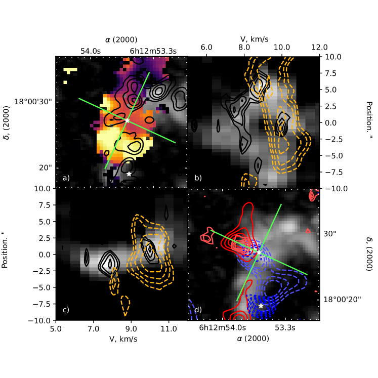
Figure 13: Spatial–kinematic structure of the clump SMA1 and its vicinity. (a) map of the C¹⁸O (2—1)intensity (background), with a map of the ammonia velocity shown in shades of yellow–violet. The black contours shows the DCO⁺ (4—3) intensity at levels of [0.4, 0.55, 0.7, 0.85, 1] Jy/beam, and the green lines show the direction of the slice of the position–velocity diagram along and perpendicular to the direction of variations in the torus velocity (panels (b) and (c), respectively). The stars show the positions of clumps. (b) and (c) Position–velocity diagram along and perpendicular to the torus. The background shows the C¹⁸O emission, the solid black contours the DCO⁺ emission, and the dashed orange contours the NH₃ (1,1)intensity. (d) Map of the C¹⁸O intensity; the solid red contours show the CO line in the red wing (pale contours are at levels of [35, 40], bold contours at levels of [16, 26] km/s), and the dashed blue contours the CO line in the blue wing (the large pale contours are at levels of [-32.5, -37.5] and the smaller contours at levels of [-5, 2] km/s

The position–velocity diagram in the (1, 1) ammonia line is presented in Fig. 7. Such a velocity profile is characteristic for a Keplerian torus (see, e.g., (Higuchi et al., 2015; Beltrán et al., 2014)) with its plane of rotation facing us, with inner and outer radii R${}_{in}\approx$ 8000 AU and R${}_{out}\approx$ 12000 AU, and a central mass of M${}_{c}~{}\approx$ 8.5 M${}_{\odot}/sin^{2}(i)$, where is the angle between the torus axis and the direction toward the observer. The shape of the ammonia emission contours and the linear radial dependence of the velocity in the inner part of the torus testify that the inclination of the torus is close to 90^∘. We constructed a position–velocity diagram similarly to the method proposed in the appendix of (Ohashi et al., 1997), but without taking into account the radial velocity. We compared the shape of the observed and model contours in the position–velocity diagram. The sizes of the outer and inner radii can also be traced in the observed position–velocity diagram, as a linear and Keplerian part of the diagram (Fig. 7). The inhomogeneous radial distribution of the ammonia intensity, and also the presence of emission at distances from the clump exceeding the outer radius of the torus, are noteworthy. Ammonia emission shifted by 0.8 km/s is observed to the north (the positive direction in Fig. 13).

Figure 13a shows that the C¹⁸O (2—1)emission between the clumps SMA1 and SMA3 is continuous spatially and also in frequency. In addition, we found that SMA1 consists of two individual clumps, which we will refer to as SMA1-NE and SMA1-SW. SMA1-NE is brighter in C¹⁸O (2—1)and has a Doppler velocity of 7 km/s, while SMA1-SW has a Doppler velocity of 9.8 km/s. According to the C¹⁸O (2—1)data, their coordinates are $\alpha$(2000)=06^h12^m53.715${}^{s}\pm$0.005^s $\delta$(2000)=18^∘00^′27.73${}^{\prime\prime}\pm$0.07^′′ abd $\alpha$(2000)=06^h12^m53.588${}^{s}\pm$0.007^s $\delta$(2000)=18^∘00^′26.2${}^{\prime\prime}\pm$0.1^′′, respectively.

3.3 Physical properties

3.3.1 Analysis of methanol observations

Emission in seven methanol lines was detected in S255N: three Class I maser lines, one Class II maser line, and three quasi-thermal lines (see Table 2). However, to all appearances, the emission of the Class II maser line is thermal.

We detected a bright source with the coordinates 06^h12^m53.70^s +18^∘00^′24.7^′ and with a velocity of 11.2 km/s in the $8_{-1}$–$7_{0}$ and $9_{-1}$–$8_{0}$ methanol transitions. The spectra of this source are shown in Fig. 14. The intensity of the lines is $\approx$7 Jy/beam, appreciably higher than the intensity in the direction of the outflow with coordinates 06^h12^m54.2^s +18^∘00^′14.9^′. This large difference in flux densities suggests that this is a maser source. Maser emission at the frequencies for these transitions has also been reported, for example, in (Val’tts, 1998; Hunter et al., 2014; Yanagida et al., 2014). The maser source is localized at the southeastern boundary of the clump SMA1 and a bipolar outflow, in both space and frequency, as can be seen in Fig. 9. We detected only one bright source, rather than the two reported in (Kurtz et al., 2004). Class I emission is also observed for the other maser sources reported in (Kurtz et al., 2004). However, the insufficient sensitivity hinders drawing unambiguous conclusions about the nature of the molecular excitation. The line is fairly narrow and shows signs of maser emission in the directions toward points 5, 6, and 7, but the shape of the spectrum in the direction of the blue part of the bipolar outflow resembles the observed profiles for the SO(6₅—5₄) and SiO(5—4) lines.

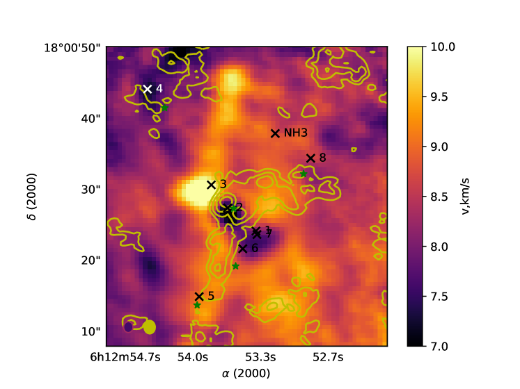
Figure 15: Map of the first moment of the CO(2—1) line. The contours show the C¹⁸O (2—1)intensity at levels of [0.4, 0.6, 0.8, 1, 1.2] K. The stars show the positions of clumps according to (Zinchenko et al., 2012), and the x’s with numbers the positions of the peak methanol emission presented in Table  3.

The positions of the points where our estimates were carried out are shown in Fig. 15. In most cases, the maximum methanol line emission is shifted relative to the center of the clumps presented in (Zinchenko et al., 2012). Methanol emission peak arranged along the line of the high-velocity outflow can also be distinguished (Wang et al., 2011). The coordinates of these maxima are presented in Table 3.

At all peaks line profiles differ from Gaussian. Two spectral peaks at $\sim$10 km/s and $\sim$6 km/s are clearly visible at positions (1) and (2), while there is no obvious division into spectral components at positions (3) and (4). The spectra at positions (1) and (2) were fitted with two Gaussians, and estimates were obtained separately for each of the components. Only one component was fitted at positions (3) and (4), at velocities of 7 and 8 km/s, respectively. Our estimates of the physical parameters of the gas are presented in Table 4.

3.3.2 Other lines

The angular separation of the two emission peaks in the CH₃CN (12₀—11₀) and C¹⁸O (2—1)lines within SMA1, identified with NE and SW, is 1.5^′′, which corresponds to a linear size in the plane of the sky of $\sim$2700 AU at a distance of 1.78 kpc(Burns et al., 2016).

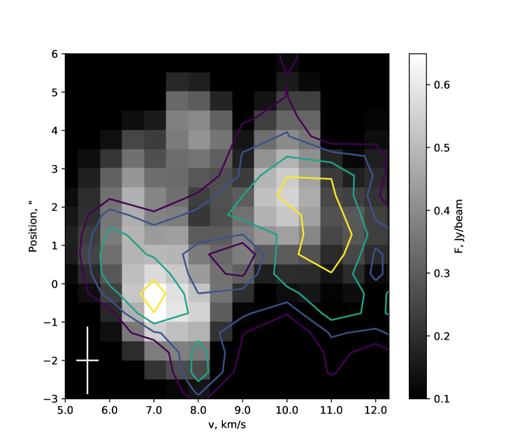
Figure 16: CH₃CN (12₀-11₀) position-velocity diagram along the direction SMA1–NE $\longrightarrow$ SMA1–SW (contours). The background shows the diagram for the C¹⁸O (2—1)line. The contours are drawn for levels of [0.07, 0.09, 0.12, 0.15, 0.2] Jy/beam. The synthesized beam of the SMA at 220.74 GHz and the width of the spectral channels are shown in the lower left corner.

Our re-reduction of the data for the (12—11) transitions (Wang et al., 2011; Zinchenko et al., 2012) leads to a separation of SMA1–NE and SMA1–SW in space and frequency, as can be seen in Fig. 16. Rotational diagrams (Martin Hernandez et al., 2008) were used to estimate the kinetic temperatures of the gas (T_k) for SMA1–NE and SMA1–SW, which were found to be 150$\pm$5K and 25${}^{+5K}_{-10K}$, respectively. We used the first five transitions of the K ladder for the estimate for SMA1–NE, and the first three transitions for SMA1–SW. The clump temperatures indicated by the analysis of the methanol data range from 20K to 100K and from 45K to 100K, respectively, close to the estimates based on the CH₃CN data. The coordinates of the IR source indicated in (Chavarria et al., 2008) are appreciably closer to SMA1–NE than to SMA1–SW.

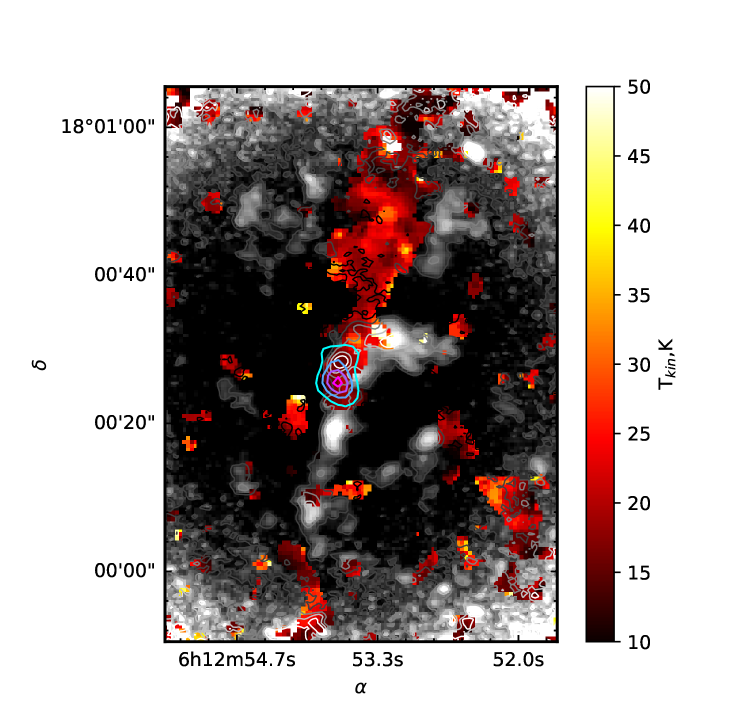
Figure 17: Map of the distribution of the kinetic temperature from the (1, 1) and (2, 2) transitions for ammonia. The shades of orange show the temperature estimates, the background and gray scale contours the C¹⁸O (2—1)intensity at levels of [0.2, 0.4, 0.6, 0.8, 1] Jy/beam, and the blue contours the integrated DCN intensity ([-3 : 19] km/s). The contours correspond to levels of [0.7, 1.5, 2.3, 3] Jy/beam m/s.

We constructed a map of the distribution of T_k based on the (2, 2) and (1, 1) ammonia lines (Fig. 17). Typical values lie in the range 10-60 K. Figure 13 shows that the ammonia emission is associated with the SW clump. Temperature estimates for SMA1–SW based on the NH₃ data are close to the estimates from the CH₃CN data, and there is no indication of hot gas associated with SMA1–NE from the ammonia data. The DCN(3—2) and DCO⁺ (4—3) emission to the south of the clumps also correlates with the region of low temperatures around SMA1—SW, but there is no DCN emission to the north. The DCO+ emission toward the north (Fig. 13) is associated with gas interacting with SMA1–NE, since it lies in space and frequency inside the part of the region of C¹⁸O (2—1)emission where there is no ammonia. The temperature of the gas in the direction of SMA2 indicated by the ammonia data grows to 54K. A cool region with a temperature of about 10K with its peak at the coordinates 6^h12^m53^s, 18^∘01^′01^′′ is also observed at the northern boundary of the map. It is striking that the temperature grows to the East and West of the ammonia emission peak in S255N–NH3, consistent with the ratio of the line intensities for these two transitions at these coordinates. We used the velocity distribution of the temperatures indicated by the ammonia data to estimate the temperature range characteristic for each fragment, presented in Table 5. The estimates of the kinetic temperatures based on the methanol and ammonia data are similar at points 5, 8, and NH₃ of Table 3.

The estimated mass of the filament joining the clumps SMA2, SMA1, and SMA3 is $\sim$8M_⊙. We used the data for the C¹⁸O (2—1)line to calculate this mass. The column density of C¹⁸O was obtained using equation (15.28) of (Rohlfs and Wilson, 2004), and the mass of gas was calculated from the abundance of this isotope of CO, 1.7$\times$10^-7 (Frerking et al., 1982).

4 Discussion

The core S255N has a fairly complex kinematic structure. To all appearances, it is being compressed by expanding HII regions(Bieging et al., 2007). The region of N₂H⁺ (3—2)emission, which traces dense gas, is located closely between the radiation-heated dust observed in the IR around the ionized regions S255 and S257. The large-scale kinematic fragments are oriented parallel to the boundary of the gas and dust envelopes, but there is no clear indication of the nature of these fragments. According to (Chavarria et al., 2008), 13 Class I and II protostellar IR sources were detected in the core. Seven large protostellar clumps with masses of 1–16 M_⊙ were also detected in the core, which are partially identified with IR sources. The presence of so many sources provides evidence of active formation of both low-mass and high-mass stars in the core. The absence of velocity profiles characteristic of compression suggests that the core has not yet made the transition to the periphery-collapse phase.

Note that the different spatial scales traced by different molecules have a mutal kinematic structure. However, several characteristic features are observed. The outer, dispersed regions of the core traced by the CO (2—1) line contain a component at a velocity of $\sim$8 km/s, which appears to be related to unperturbed gas surrounding the core. In addition, three directions for variations of the velocity can be distinguished from the center toward the northeast, the southwest, and the southeast. These last two correspond to the directions toward the ionized regions S255 and S257, suggesting that some kinematic fragments may come about as a consequence of an external interaction. Velocity slices for molecules tracing dense gas (NH₃ (1,1), N₂H⁺ (3—2), C¹⁸O (2—1)) resemble the section in the CO(2—1) line, apart from the component at $\sim$8 km/s, and also the region around the clumps. However, not all of the gas fragments can be formed by external factors. In particular, an extended structure connecting the clumps SMA1, SMA2 and SMA3 and kinematically related to these clumps can be seen in the C¹⁸O line. In addition, two fragments are observed along the line of sight in the direction of the blue wing of the bipolar outflow from SMA1 in the N₂H⁺ and NH₃ lines; one of these is not associated with dispersed gas of the core, since it is not represent in the CO(2—1) line.

The N₂H⁺ NH₃ C¹⁸O and SO data suggest that the matter in the core is distributed fairly inhomogeneously, with kinematically distinct interacting gas components being present. Clumps are not present in all of these, as can be seen in the velocity in Fig.6.

The dense, compact gas observed in C¹⁸O (2—1)has an elongated structure. This emission is appreciably correlated with the emission in the N₂H⁺ (3—2)line, but the portion that is not is located in the region of overlap of the kinematic fragments of the core. Figure 13 shows that SMA1 is surrounded by matter mainly to the north and south, as can be seen in the position–velocity diagram. The line spectrum at the currently available resolution varies smoothly, separating into two components toward SMA1 (NE and SW) – a sign of interaction of the elongated structure with the clumps. It is also important that the emission at 8-9 km/s is appreciably weaker at the center of SMA than in the filament. This may indicate that a large fraction of the filament gas in the vicinity of the clumps is interacting with this filament (Fig. 9).

The C¹⁸O, CH₃CN, CH₃OH and DCO⁺ data unambiguously indicate the presence of two clumps, which were not resolved earlier and have been interpreted as the object S255N SMA1. We have also continued to use the notation SMA1 when referring to the most evolved, kinematically rich central region of the core. It is noteworthy that the mean velocity of the detected giant torus coincides with the velocity of SMA1–SW, although its size is much larger than the distance between NE and SW (in the plane of the sky). Compact regions of DCO⁺ emission that are kinematically related to both clumps are observed. An appreciably fraction of the DCO⁺ emission is located outside the clumps, but inside the torus, correlating with C¹⁸O (Fig. 13). The NE clump is associated with a bipolar outflow (Fig. 18) observed in the wings of CO(2—1), SO(6₅—5₄) and SiO(5—4) lines, and also with a water maser (Cyganowski et al., 2007) and methanol masers from (Kurtz et al., 2004) and detected by us. Regions of DCO⁺ emission are present in the gas interacting with NE. This effect is not observed for SW. It is noteworthy that SW is located practically on the line of the bipolar outflow from NE. This feature could quite plausibly result due to the action of the outflow on the gas in the core. However, the relevance of the torus in this picture remains unclear. Signs of the torus are also observed in the C¹⁸O (2—1)data. Asymmetry of the CO velocity profiles relative to NE can be traced in Fig. 18.

Analysis of the position–velocity diagram in the C¹⁸O, SO, NH₃ and DCO⁺ lines suggests that the torus traced in the ammonia lines is related to the accretion of the more extended, dense material of the elongated, filament-like structure onto the two young protostellar clumps. The position–velocity diagram in the C¹⁸O line in the vicinity of SMA1 indicates an active transfer of matter between the clumps and the ambient gas in the rotational plane of the torus, with quasi-Keplerian radial profiles (Figs. 13 a,b,c).

The detected torus is one of several dozen known disk-like objects around massive protostars (Beuther et al., 2017; Zinchenko et al., 2015; Beltrán and de Wit, 2016; Quanz et al., 2010; Chini et al., 2006; Sako et al., 2005). However, a large fraction of known disks have smaller sizes or are located around less massive protostars. Tori that are larger than the disks and have appreciable thicknesses are also known (Beltrán et al., 2014; Boley et al., 2013; Sollins et al., 2005; Beltrán et al., 2011a, b; Higuchi et al., 2015). The object G28.20-0.05 is closest in terms of its size and physical parameters. The object we have discovered is large ($\sim$24 000 AU in diameter, as opposed to $\leq$12 000 AU for G28.20-0.05). The two regions both host an ultracompact HII region. The temperatures for the two objects estimated from ammonia lines are similar(Sollins et al., 2005). However, warmer, chemically rich torus-like rotating structures are also observed (Beltrán et al., 2011a, b). The presence of a dust component in a similar object is also known (Quanz et al., 2010). No signs of such a component have been detected in the case of S255N SMA1 (Miralles et al., 1997; Wang et al., 2011; Zinchenko et al., 2012).

Theoretical models predict the appearance of torus-like objects that are gravitationally unstable (Cesaroni et al., 2007), together with an important role for the late accretion of matter onto a protostar as a transitional structure (Kratter et al., 2010). The detection of a torus is consistent with the hypothesis of the formation of massive stars via disk accretion (Balbus and Hawley, 1998; Krumholz et al., 2009). Observations of the region with better angular resolution and simultaneously higher sensitivity are needed for estimates of the accretion rates and detailed studies of the interaction of the torus and the ambient gas.

5 Conclusion

We have considered the kinematic structure of the S255N core on various spatial scales, from the outer layers of the core to dense clumps in the core. Our analysis has led to the following discoveries.

1. The core does not show characteristic signs of either isotropic collapse or rotation. Overall, the large-scale motions are in agreement with those described in (Pirogov et al., 2003), however, the structure of the core is very inhomogeneous.

2. At least five extended parts of the core are observed, within which the gas velocities are similar.

3. Large fragments of the core ($\sim$1/3 the size of the core itself) are oriented parallel to the boundaries of the HII regions S255 and S257.

4. A large fraction of smaller fragments is associated with the SMA1 clump. One of these fragments is located to the southeast of SMA1 along the line of a bipolar outflow, and is elongated along this outflow. Another fragment connecting the clumps SMA3-2-1 is also elongated, and it is fairly massive ($\sim$ 8M_⊙).

5. We have detected a circumstellar torus rotating around SMA1, with inner radius R${}_{in}\approx$8000 AU and outer radius R${}_{out}\approx$ 12000 AU. The rotation profile is characteristic of Keplerian motion around a central mass of $\sim$ 8.5/$sin^{2}(i)$ M_⊙.

6. SMA1 is spatially resolved into two separated clumps, NE and SW. They actively interact with the torus and a filament. One of the clumps is fairly cool ($\sim$25 K), while the other is much hotter ($\sim$150 K). The bipolar outflow is associated with the hot source.

7. A Class I maser source was detected in the CH₃OH $4_{2}$–$3_{1}$, $8_{-1}$–$7_{0}$ and $9_{-1}$–$8_{0}$ lines, with coordinates $\alpha$(2000)=06^h12^m53.69^s $\delta$(2000)=+18^∘00^′25.0^′ and radial velocity $\approx$11.2 km/s. This source is located at the northeast boundary of the bipolar outflow from SMA1–NE.

8. The kinetic temperature and number density of the gas in the clumps and outflows vary in the ranges 15–220 K and 10⁴ – 10⁵ cm^-3 . The filling factor for the sources in the outflows is low, suggesting strong fragmentation of the gas.

9. The temperature of the gas in the core is distributed inhomogeneously both in terms of the parameters of different fragments and inside the fragments themselves. Fragments that do not contain clumps have lower temperatures and smaller temperature ranges.

10. We detected a clump with the coordinates (7^′′, -34^′′ ) relative to SMA1, together with a related high-velocity outflow.

6 Acknowledgments

We thank L.E. Pirogov and A.V. Lapinov for useful discussions of material and methods. We also thank the referee for thoughtful comments that have helped improve this paper.

This work was supported by the Russian Foundation for Basic Research (grants 16-32-00873, 16-02-00761, 15-02-06098), the Russian Science Foundation (grant 17-12-01256), decree No. 211 of the Government of the Russian Federation (contract 02.A03.21.0006), and the Ministry of Education and Science of the Russian Federation (grant RK AAAA-A17-117030310283-7).

petez@ipfran.ru

Table 1: List of analyzed lines. The symbol ^∗ denotes data obtained in the extended and compact configurations. SMA+IRAM and SMA^∗+IRAM denote the combined data

Molecule, transition	Frequency, GHz	Telescope
NH3 (1,1)	23.69	VLA
NH3 (2,2)	23.72	VLA
CH3OH-E ($5_{1}$—$4_{2}$)	216.94	SMA
SiO (5—4)	217.10	SMA+IRAM
CO (2—1)	217.23	SMA∗+IRAM
DCN (3—2)	217.23	SMA
CH3OH-E ($4_{2}$—$3_{1}$)	218.44	SMA
C18O (2—1)	219.65	SMA∗
CH3CN (12—11)	220.59	SMA*
CH3OH-E ($8_{0}$—$7_{1}$)	220.07	SMA
CH3OH-E ($8_{-1}$—$7_{0}$)	229.75	SMA
CH3OH-E ($3_{-2}$—$4_{-1}$)	230.02	SMA
CH3OH ($9_{-1}$—$8_{0}$)	278.30	SMA
N2H+ (3—2)	279.51	SMA+IRAM
DCO+ (4—3)	288.14	SMA
SO (65—54)	288.51	SMA∗
C34S (6—5)	289.20	SMA
CH3OH-E ($6_{0}$—$5_{0}$)	289.93	SMA

Table 2: Methanol lines detected at 216–290 GHz used to estimate physical conditions

Transition	Frequency, GHz	$E_{low}$,K	$E_{up}$,K	Comments
$5_{1}$—$4_{2}$	216.945	37	47	Class II maser
$4_{2}$—$3_{1}$	218.440	27	37	Class I maser
$8_{0}$—$7_{1}$	220.078	78	88
$8_{-1}$—$7_{0}$	229.758	70	81	Class I maser
$3_{-2}$—$4_{-1}$	230.027	20	31
$9_{-1}$—$8_{0}$	278.304	88	102	Class I maser
$6_{0}$—$5_{0}$	289.939	40	53

Table 3: Coordinates of methanol emission peaks

N	RA(2000)	DEC(2000)	Nearest object
1	6:12:53.42	18:00:23.65	Near SMA1
2	6:12:53.70	18:00:26.90	2 and 3
3	6:12:53.86	18:00:30.15	5 and 6
4	6:12:54.49	18:00:43.65	SMA4
5	6:12:53.98	18:00:14.40	SMA5, 7
6	6:12:53.55	18:00:21.15	SMA3
7	6:12:53.41	18:00:23.15	SMA1
8	6:12:52.88	18:00:33.90	SMA2
NH3	6:12:53.23	18:00:37.40	NH3 (1,1) peak

Table 4: Physical parameters of gas from the fitting. 1$\sigma$ parameter range shown in parantheses. At position (4), the density range of 3–9 corresponds to the entire range in the database (model gives no constraints). $ff$ is the beam filling factor. Ntr is the number of model parameters. The column ”!” gives the number of lines with non-zero intensities at the indicated positions

N	VLSR(km/s)	Tk,K	lg(Nm/$\Delta$V)	lg(n)[H2]	lg(N${}_{CH_{3}OH}$/N${}_{H_{2}}$)	ff	$\chi^{2}$/Ntr	!
1	9.8	45(40-100)	10.50(10.00-11.00)	6.0(¡7.5)	-6	12.45	0.90	7
1	5.6	50(¿25)	10.00( 9.50-10.50)	6.5(3.0-9.0)	-8	1.15	0.16	7
2	7.6	30(¿20)	11.25(10.00-12.00)	3.5(¡7.0)	-6	11	1.9	6
2	11.3	60(45-100)	9.75( 9.50-10.00)	6.0(5.75-6.75)	-6	77	4.4	5
3	7.1	40(30-160)	11.25(10.5-12.5)	6.0(¡7.5)	-6	4	0.9	7
4	7.8	120(¿45)	9.50(9.25-10.0)	6.5(3.0-9.0)	-6	69.7	4.4	4
6	9.2	85(50-200)	9.0(8.75-9.25)	6.0(¿5.5)	-6	67.2	1.32	4
7	9.7	60(40-120)	9.75(9.5-10.0)	6.0(5.5-7.0)	-6	65.02	5.09	6
5	7.5	165(¿50)	8.00(¡8.5)	6.0(5.5-7.5)	-6	99.0	2.24	2
6	4.9	50(10-220)	9.25(¡9.0)	6.0(3-9)	-6	55.8	0.50	5
7	5.4	55(40-120)	9.50(9.25-9.75)	6.0(5.5-7.0)	-6	65.41	2.22	6
8	4.7	20(¡30)	11.25(8-13)	3.5(3-9)	-7	9.35	1.05	3
NH3	9.5	15(¡25)	11.25(11-12)	5.0(3-9)	-8	54.8	1.06	3
NH3	7.6	15(¡25)	11.50(11.25-11.75)	6.5(¿5.5)	-8	77.9	2.60	4

Table 5: Parameters of kinematic fragment of the core. The range of kinetic temperatures in the fragments was obtained from the (1, 1) and (2, 2) transitions of ammonia

Fragment number	Velocity, km/s	Tk, K	Comments
1	$\sim$7.2	10-25	SMA5
2	$\sim$7.8	10-40	SMA1, SMA4
3	$\sim$8.3	6-30,80	SMA3
4	$\sim$9.1	10-53	SMA2, SMA6
5	$\sim$10.3	12-23	Oriented toward the outflow from SMA1 SMA1

Figure 7: Position–velocity diagram in the NH₃ line. A model of a Keplerian torus with R_out=0.06 pc, R_in=0.04 pc, M_c=8.5 M_⊙ is shown in the background. The contours show the main component of the hyperfine structure of the ammonia line at levels of [2.8, 3.2, 3.7, 4.3, 5.0] K, and the x’s the velocities derived using the kNN method in the same line, with the uncertainties indicated by the horizontal segments.

Figure 9: Spectral slice along the path shown in Fig. 8. The background shows the combined IRAM + SMA intensity for the CO(2—1) line, the red contours the N₂H⁺ (3—2)intensity at levels of [6, 9, 12, 16, 23, 31, 43, 58] Jy/beam, the blue dashed contours the emission in the SO (6₅—5₄)line at levels of [0.18, 0.2, 0.35, 0.5, 0.7, 1] Jy/beam, and the filled contours in shades of blue–violet the intensity in the C¹⁸O (2—1)line at levels of [0.17, 0.23, 0.3, 0.38, 0.49] Jy/beam. The vertical dot–dashed lines and numbers indicate the positions of kinematic components identified in Fig. 6.

Figure 10: Spectral slice along the clumps SMA3-1-2. The background shows the CO(2—1) intensity, the filled contours in shades of blue–violet the C 18 O(2–1) emission at levels of [0.2, 0.3, 0.4, 0.6, 0.8] Jy/beam, the dashed blue contours the SO (6₅—5₄)emission at levels of [0.1, 0.14, 0.18, 0.2, 0.28, 0.35, 0.44, 0.55] Jy/beam, and the red contours the DCO⁺ (4—3) emission at levels of [0.37, 0.41, 0.45, 0.49, 0.53, 0.57, 0.62, 0.68] Jy/beam.

Figure 11: N₂H⁺ (3—2)(IRAM + SMA), DCO⁺ (4—3), and CO(2—1) spectra in the direction of the peak DCO⁺ emission, (-7^′′, 34^′′) relative to the phase center.

Figure 12: Map of the Doppler velocity from the fit to the NH₃ (1,1)line (color scale). The contours show the integrated intensity in the CO(2—1) wings, associated with the bipolar outflow, at levels of [26.5, 35.5] (solid contours) and [-18.5, -8] (dashed contours). The sizes of the VLA (outer ellipse) and SMA (inner ellipse) antenna beams are shown in the lower left-hand corner. The star shows the position of the clump SMA1, and the $\times$ and + symbols the positions of maser sources according to (Kurtz et al., 2004) (Class I methanol) and (Cyganowski et al., 2007) (H₂O).

Figure 14: Methanol spectra for the transitions $8_{-1}$–$7_{0}$, $9_{-1}$–$8_{0}$ (lower, shifted by 8 Jy/beam), in the direction of the point with coordinates 06^h12^m53.69^s +18^∘00^′25.0^′ (J2000) (the maser spot, thin curves) and 06^h12^m54.2^s +18^∘00^′14.9^′ (J2000) (the bipolar outflow, bold curves).

Figure 18: Position–velocity diagram along the bipolar outflow, denoted by the blue line in Fig. 13(a). The background shows the combined data in the CO (2—1) line, the red contours the interferometric data in this same line, the dashed blue contours the combined data in the SiO (5—4) line, and the filled contours in shades of blue–violet the data for the C¹⁸O (2—1)line. The filled yellow circles show the positions of methanol masers according to (Kurtz et al., 2004) and Section 3.3.1, and the filled yellow square the position of the water maser presented in (Cyganowski et al., 2007).

References

- Mapelli (2017) M. Mapelli. Rotation in young massive star clusters. Mon. Not. R. Astron. Soc, 467:3255–3267, May 2017. doi: 10.1093/mnras/stx304.
- Sokolov et al. (2017) V. Sokolov, K. Wang, J. E. Pineda, P. Caselli, J. D. Henshaw, J. C. Tan, F. Fontani, I. Jiménez-Serra, and W. Lim. Temperature structure and kinematics of the IRDC G035.39-00.33. Astron. Astrophys, 606:A133, October 2017. doi: 10.1051/0004-6361/201630350.
- Richardson et al. (1985) K. J. Richardson, G. J. White, G. Gee, M. J. Griffin, C. T. Cunningham, P. A. R. Ade, and L. W. Avery. Submillimetre line and continuum observations of the S255 molecular cloud. Mon. Not. R. Astron. Soc, 216:713–733, October 1985. doi: 10.1093/mnras/216.3.713.
- Pirogov et al. (2003) L. Pirogov, I. Zinchenko, P. Caselli, L. E. B. Johansson, and P. C. Myers. N2H+(1-0) survey of massive molecular cloud cores. Astron. Astrophys, 405:639–654, July 2003. doi: 10.1051/0004-6361:20030659.
- Bieging et al. (2007) J. H. Bieging, W. L. Peters, B. V. Vilaro, K. Schlottman, and C. Kulesa. Sequential star formation in the Sh 254-258 molecular cloud: HHT maps of CO J=3-2 and 2-1 emission. In B. G. Elmegreen and J. Palous, editors, Triggered Star Formation in a Turbulent ISM, volume 237 of IAU Symposium, page 396, 2007. doi: 10.1017/S1743921307001846.
- Wang et al. (2011) Y. Wang, H. Beuther, A. Bik, T. Vasyunina, Z. Jiang, E. Puga, H. Linz, J. A. Rodón, T. Henning, and M. Tamura. Different evolutionary stages in the massive star-forming region S255 complex. Astron. Astrophys, 527:A32, March 2011. doi: 10.1051/0004-6361/201015543.
- Ojha et al. (2011) D. K. Ojha, M. R. Samal, A. K. Pandey, B. C. Bhatt, S. K. Ghosh, S. Sharma, M. Tamura, V. Mohan, and I. Zinchenko. Star Formation Activity in the Galactic H II Complex S255-S257. Astrophys. J, 738:156, September 2011. doi: 10.1088/0004-637X/738/2/156.
- Zinchenko et al. (2012) I. Zinchenko, S.-Y. Liu, Y.-N. Su, S. Kurtz, D. K. Ojha, M. R. Samal, and S. K. Ghosh. A Multi-wavelength High-resolution study of the S255 Star-forming Region: General Structure and Kinematics. Astrophys. J, 755:177, August 2012. doi: 10.1088/0004-637X/755/2/177.
- Kurtz et al. (2004) S. Kurtz, P. Hofner, and C. V. Álvarez. A Catalog of CH3OH 70-61 A+ Maser Sources in Massive Star-forming Regions. Astrophys. J. Suppl. Ser, 155:149–165, November 2004. doi: 10.1086/423956.
- Zinchenko et al. (2009) I. Zinchenko, P. Caselli, and L. Pirogov. Chemical differentiation in regions of high-mass star formation - II. Molecular multiline and dust continuum studies of selected objects. Mon. Not. R. Astron. Soc, 395:2234–2247, June 2009. doi: 10.1111/j.1365-2966.2009.14687.x.
- Minier et al. (2007) V. Minier, N. Peretto, S. N. Longmore, M. G. Burton, R. Cesaroni, C. Goddi, M. R. Pestalozzi, and P. André. Anatomy of the S255-S257 complex - triggered high-mass star formation. In B. G. Elmegreen and J. Palous, editors, Triggered Star Formation in a Turbulent ISM, volume 237 of IAU Symposium, pages 160–164, 2007. doi: 10.1017/S1743921307001391.
- Kurtz et al. (1994) S. Kurtz, E. Churchwell, and D. O. S. Wood. Ultracompact H II regions. 2: New high-resolution radio images. Astrophys. J. Suppl. Ser, 91:659–712, April 1994. doi: 10.1086/191952.
- Cyganowski et al. (2007) C. J. Cyganowski, C. L. Brogan, and T. R. Hunter. Evidence for a Massive Protocluster in S255N. Astron. J, 134:346–358, July 2007. doi: 10.1086/518740.
- Burns et al. (2016) R. A. Burns, T. Handa, T. Nagayama, K. Sunada, and T. Omodaka. H2O masers in a jet-driven bow shock: episodic ejection from a massive young stellar object. Mon. Not. R. Astron. Soc, 460:283–290, July 2016. doi: 10.1093/mnras/stw958.
- Sault et al. (1995) R. J. Sault, P. J. Teuben, and M. C. H. Wright. A Retrospective View of MIRIAD. In R. A. Shaw, H. E. Payne, and J. J. E. Hayes, editors, Astronomical Data Analysis Software and Systems IV, volume 77 of Astronomical Society of the Pacific Conference Series, page 433, 1995.
- Schwab (1984) F. R. Schwab. Relaxing the isoplanatism assumption in self-calibration; applications to low-frequency radio interferometry. Astron. J, 89:1076–1081, July 1984. doi: 10.1086/113605.
- Müller et al. (2005) H. S. P. Müller, F. Schlöder, J. Stutzki, and G. Winnewisser. The Cologne Database for Molecular Spectroscopy, CDMS: a useful tool for astronomers and spectroscopists. Journal of Molecular Structure, 742:215–227, May 2005. doi: 10.1016/j.molstruc.2005.01.027.
- Knuth (2006) K. H. Knuth. Optimal Data-Based Binning for Histograms. ArXiv Physics e-prints, May 2006.
- Scargle et al. (2013) J. D. Scargle, J. P. Norris, B. Jackson, and J. Chiang. Studies in Astronomical Time Series Analysis. VI. Bayesian Block Representations. Astrophys. J, 764:167, February 2013. doi: 10.1088/0004-637X/764/2/167.
- Astropy Collaboration et al. (2013) Astropy Collaboration, T. P. Robitaille, E. J. Tollerud, P. Greenfield, M. Droettboom, E. Bray, T. Aldcroft, M. Davis, A. Ginsburg, A. M. Price-Whelan, W. E. Kerzendorf, A. Conley, N. Crighton, K. Barbary, D. Muna, H. Ferguson, F. Grollier, M. M. Parikh, P. H. Nair, H. M. Unther, C. Deil, J. Woillez, S. Conseil, R. Kramer, J. E. H. Turner, L. Singer, R. Fox, B. A. Weaver, V. Zabalza, Z. I. Edwards, K. Azalee Bostroem, D. J. Burke, A. R. Casey, S. M. Crawford, N. Dencheva, J. Ely, T. Jenness, K. Labrie, P. Lian Lim, F. Pierfederici, A. Pontzen, A. Ptak, B. Refsdal, M. Servillat, and O. Streicher. Astropy: A community Python package for astronomy. Astron. Astrophys, 558:A33, October 2013. doi: 10.1051/0004-6361/201322068.
- Altman (1992) N. S. Altman. An introduction to kernel and nearest-neighbor nonparametric regression. The American Statistician, 46(3):175–185, 1992. doi: 10.1080/00031305.1992.10475879. URL http://www.tandfonline.com/doi/abs/10.1080/00031305.1992.10475879.
- Salii (2006) S. V. Salii. A database for estimating the physical parameters of molecular clouds by the intensities of the radio lines of methanol. Star Formation in the Galaxy and Beyond, pages 146–151, 2006. URL ttp://hdl.handle.net/10995/46181.
- Cragg et al. (2005) D. M. Cragg, A. M. Sobolev, and P. D. Godfrey. Models of class II methanol masers based on improved molecular data. Mon. Not. R. Astron. Soc, 360:533–545, June 2005. doi: 10.1111/j.1365-2966.2005.09077.x.
- Miralles et al. (1997) M. P. Miralles, L. Salas, I. Cruz-González, and S. Kurtz. Discovery of Jets and HH-like Objects near the S255 IR Complex. Astrophys. J, 488:749–759, October 1997. doi: 10.1086/304713.
- Chavarria et al. (2008) L. A. Chavarria, L. E. Allen, J. L. Hora, C. M. Brunt, and G. G. Fazio. Spitzer Observations of the Massive Star-forming Complex S254-S258: Structure and Evolution. Astrophys. J, 682:445-462, July 2008. doi: 10.1086/588810.
- Higuchi et al. (2015) A. E. Higuchi, T. Hasegawa, K. Saigo, P. Sanhueza, and J. O. Chibueze. Sgr B2(N): A Bipolar Outflow and Rotating Hot Core Revealed by ALMA. Astrophys. J, 815:106, December 2015. doi: 10.1088/0004-637X/815/2/106.
- Beltrán et al. (2014) M. T. Beltrán, Á. Sánchez-Monge, R. Cesaroni, M. S. N. Kumar, D. Galli, C. M. Walmsley, S. Etoka, R. S. Furuya, L. Moscadelli, T. Stanke, F. F. S. van der Tak, S. Vig, K.-S. Wang, H. Zinnecker, D. Elia, and E. Schisano. Filamentary structure and Keplerian rotation in the high-mass star-forming region G35.03+0.35 imaged with ALMA. Astron. Astrophys, 571:A52, November 2014. doi: 10.1051/0004-6361/201424031.
- Ohashi et al. (1997) N. Ohashi, M. Hayashi, P. T. P. Ho, and M. Momose. Interferometric Imaging of IRAS 04368+2557 in the L1527 Molecular Cloud Core: A Dynamically Infalling Envelope with Rotation. Astrophys. J, 475:211–223, January 1997. doi: 10.1086/303533.
- Val’tts (1998) I. E. Val’tts. The unusual methanol maser 345.01+1.79. Astronomy Letters, 24:788–794, November 1998.
- Hunter et al. (2014) T. R. Hunter, C. L. Brogan, C. J. Cyganowski, and K. H. Young. Subarcsecond Imaging of the NGC 6334 I(N) Protocluster: Two Dozen Compact Sources and a Massive Disk Candidate. Astrophys. J, 788:187, June 2014. doi: 10.1088/0004-637X/788/2/187.
- Yanagida et al. (2014) Takahiro Yanagida, Takeshi Sakai, Tomoya Hirota, Nami Sakai, Jonathan B. Foster, Patricio Sanhueza, James M. Jackson, Kenji Furuya, Yuri Aikawa, and Satoshi Yamamoto. Alma observations of the irdc clump g34.43+00.24 mm3: 278 ghz class i methanol masers. The Astrophysical Journal Letters, 794(1):L10, 2014. URL http://stacks.iop.org/2041-8205/794/i=1/a=L10.
- Martin Hernandez et al. (2008) N. L. Martin Hernandez, A. Bik, E. Puga, D. E. A. Nürnberger, and L. Bronfman. Spatially resolved near-infrared spectroscopy of the massive star-forming region IRAS 19410+2336. Astron. Astrophys, 489:229–243, October 2008. doi: 10.1051/0004-6361:200810336.
- Rohlfs and Wilson (2004) K. Rohlfs and T. L. Wilson. Tools of radio astronomy. Springer, 2004.
- Frerking et al. (1982) M. A. Frerking, W. D. Langer, and R. W. Wilson. The relationship between carbon monoxide abundance and visual extinction in interstellar clouds. Astrophys. J, 262:590–605, November 1982. doi: 10.1086/160451.
- Beuther et al. (2017) H. Beuther, A. J. Walsh, K. G. Johnston, T. Henning, R. Kuiper, S. N. Longmore, and C. M. Walmsley. Fragmentation and disk formation in high-mass star formation: The ALMA view of G351.77-0.54 at 0.06” resolution. Astron. Astrophys, 603:A10, June 2017. doi: 10.1051/0004-6361/201630126.
- Zinchenko et al. (2015) I. Zinchenko, S.-Y. Liu, Y.-N. Su, S. V. Salii, A. M. Sobolev, P. Zemlyanukha, H. Beuther, D. K. Ojha, M. R. Samal, and Y. Wang. The Disk-outflow System in the S255IR Area of High-mass Star Formation. Astrophys. J, 810:10, September 2015. doi: 10.1088/0004-637X/810/1/10.
- Beltrán and de Wit (2016) M. T. Beltrán and W. J. de Wit. Accretion disks in luminous young stellar objects. The Astronomy and Astrophysics Review, 24:6, January 2016. doi: 10.1007/s00159-015-0089-z.
- Quanz et al. (2010) S. P. Quanz, H. Beuther, J. Steinacker, H. Linz, S. M. Birkmann, O. Krause, T. Henning, and Q. Zhang. A Large, Massive, Rotating Disk Around an Isolated Young Stellar Object. Astrophys. J, 717:693–707, July 2010. doi: 10.1088/0004-637X/717/2/693.
- Chini et al. (2006) R. Chini, V. H. Hoffmeister, M. Nielbock, C. M. Scheyda, J. Steinacker, R. Siebenmorgen, and D. Nürnberger. A Remnant Disk around a Young Massive Star. Astrophys. J. Lett, 645:L61–L64, July 2006. doi: 10.1086/505862.
- Sako et al. (2005) S. Sako, T. Yamashita, H. Kataza, T. Miyata, Y. K. Okamoto, M. Honda, T. Fujiyoshi, H. Terada, T. Kamazaki, Z. Jiang, T. Hanawa, and T. Onaka. No high-mass protostars in the silhouette young stellar object M17-SO1. Nature, 434:995–998, April 2005. doi: 10.1038/nature03471.
- Boley et al. (2013) P. A. Boley, H. Linz, R. van Boekel, T. Henning, M. Feldt, L. Kaper, C. Leinert, A. Müller, I. Pascucci, M. Robberto, B. Stecklum, L. B. F. M. Waters, and H. Zinnecker. The VLTI/MIDI survey of massive young stellar objects . Sounding the inner regions around intermediate- and high-mass young stars using mid-infrared interferometry. Astron. Astrophys, 558:A24, October 2013. doi: 10.1051/0004-6361/201321539.
- Sollins et al. (2005) P. K. Sollins, Q. Zhang, E. Keto, and P. T. P. Ho. An Infalling Torus of Molecular Gas around the Ultracompact H II Region G28.20-0.05. Astrophys. J, 631:399–410, September 2005. doi: 10.1086/432503.
- Beltrán et al. (2011a) M. T. Beltrán, R. Cesaroni, R. Neri, and C. Codella. Rotating toroids in G10.62-0.38, G19.61-0.23, and G29.96-0.02. Astron. Astrophys, 525:A151, January 2011a. doi: 10.1051/0004-6361/201015049.
- Beltrán et al. (2011b) M. T. Beltrán, R. Cesaroni, Q. Zhang, R. Galván-Madrid, H. Beuther, C. Fallscheer, R. Neri, and C. Codella. Molecular outflows and hot molecular cores in G24.78+0.08 at sub-arcsecond angular resolution. Astron. Astrophys, 532:A91, August 2011b. doi: 10.1051/0004-6361/201117200.
- Cesaroni et al. (2007) R. Cesaroni, D. Galli, G. Lodato, C. M. Walmsley, and Q. Zhang. Disks Around Young O-B (Proto)Stars: Observations and Theory. Protostars and Planets V, pages 197–212, 2007.
- Kratter et al. (2010) K. M. Kratter, C. D. Matzner, M. R. Krumholz, and R. I. Klein. On the Role of Disks in the Formation of Stellar Systems: A Numerical Parameter Study of Rapid Accretion. Astrophys. J, 708:1585–1597, January 2010. doi: 10.1088/0004-637X/708/2/1585.
- Balbus and Hawley (1998) S. A. Balbus and J. F. Hawley. Instability, turbulence, and enhanced transport in accretion disks. Reviews of Modern Physics, 70:1–53, January 1998. doi: 10.1103/RevModPhys.70.1.
- Krumholz et al. (2009) M. R. Krumholz, R. I. Klein, C. F. McKee, S. S. R. Offner, and A. J. Cunningham. The Formation of Massive Star Systems by Accretion. Science, 323:754, February 2009. doi: 10.1126/science.1165857.