Zoom-SVD: Fast and Memory Efficient Method for
Extracting Key Patterns in an Arbitrary Time Range

Abstract.

Given multiple time series data, how can we efficiently find latent patterns in an arbitrary time range? Singular value decomposition (SVD) is a crucial tool to discover hidden factors in multiple time series data, and has been used in many data mining applications including dimensionality reduction, principal component analysis, recommender systems, etc. Along with its static version, incremental SVD has been used to deal with multiple semi-infinite time series data and to identify patterns of the data. However, existing SVD methods for the multiple time series data analysis do not provide functionality for detecting patterns of data in an arbitrary time range: standard SVD requires data for all intervals corresponding to a time range query, and incremental SVD does not consider an arbitrary time range.

In this paper, we propose Zoom-SVD, a fast and memory efficient method for finding latent factors of time series data in an arbitrary time range. Zoom-SVD incrementally compresses multiple time series data block by block to reduce the space cost in storage phase, and efficiently computes singular value decomposition (SVD) for a given time range query in query phase by carefully stitching stored SVD results. Through extensive experiments, we demonstrate that Zoom-SVD is up to $15\times$ faster, and requires $15\times$ less space than existing methods. Our case study shows that Zoom-SVD is useful for capturing past time ranges whose patterns are similar to a query time range.

1. Introduction

Given multiple time series data (e.g., measurements from multiple sensors) and a time range (e.g., 1:00 am - 3:00 am yesterday), how can we efficiently discover latent factors of the time series in the range? Revealing hidden factors in time series is important for analysis of patterns and tendencies encoded in the time series data. Singular value decomposition (SVD) effectively finds hidden factors in data, and has been extensively utilized in many data mining applications such as dimensionality reduction (Ravi Kanth et al., 1998), principal component analysis (PCA) (Jolliffe, 2002; Wall et al., 2003), data clustering (Simek et al., 2004; Osiński et al., 2004), tensor analysis (Sael et al., 2015; Jeon et al., 2015; Jeon et al., 2016b; Jeon et al., 2016a; Park et al., 2016; Oh et al., 2018), graph mining (Kang et al., 2012; Tong et al., 2006; Kang et al., 2011, 2014) and recommender systems (Koren et al., 2009; Park et al., 2017). SVD has been also successfully applied to stream mining tasks (Wall et al., 2003; Spiegel et al., 2011) in order to analyze time series data.

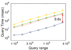
(a) Query time of the Activity dataset

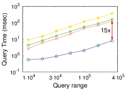
(b) Query time of the Gas dataset

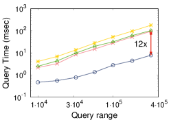
(c) Query time of the London dataset

Figure 1. Query time of Zoom-SVD compared to other SVD methods. The starting point $t_{s}$ and the ending point $t_{e}$ are arbitrarily chosen, and we increase time range $t_{e}-t_{s}$ from $10^{4}$ to $3.2\times 10^{5}$. (a) The query time of Zoom-SVD is up to $9.6\times$ faster than that of the second best method in Activity dataset. (b) Zoom-SVD is up to $15\times$ faster than the second best method in the query phase of Gas dataset. (c) Zoom-SVD is up to $12\times$ faster than the second best method in the query phase of London dataset.

However, methods based on standard SVD (Brand, 2003; Ross et al., 2008; Zadeh et al., 2016; Halko et al., 2011) are not suitable for finding latent factors in an arbitrary time range since the methods have an expensive computational cost, and they have to store all the raw data. This limitation makes it difficult to investigate patterns of a time range in stream environment even if it is important to analyze a specific past event or find recurring patterns in time series (Papadimitriou and Yu, 2006). A naive approach for a time range query on time series is to store all of the arrived data and apply SVD to the data, but this approach is inefficient since it requires huge storage space, and the computational cost of SVD for a long time range query is expensive.

In this paper, we propose Zoom-SVD (Zoomable SVD), an efficient method for revealing hidden factors of multiple time series in an arbitrary time range. With Zoom-SVD, users can zoom-in to find patterns in a specific time range of interest, or zoom-out to extract patterns in a wider time range. Zoom-SVD comprises two phases: storage phase and query phase. Zoom-SVD considers multiple time series as a set of blocks of a fixed length. In the storage phase, Zoom-SVD carefully compresses each block using SVD and low-rank approximation to reduce storage cost and incrementally updates the most recent block of a newly arrived data. In the query phase, Zoom-SVD efficiently computes the SVD results in a given time range based on the compressed blocks. Through extensive experiments with real-world multiple time series data, we demonstrate the effectiveness and the efficiency of Zoom-SVD compared to other methods as shown in Figure 1. The main contributions of this paper are summarized as follows:

• Algorithm. We propose Zoom-SVD, an efficient method for extracting key patterns from multiple time series data in an arbitrary time range.

• Analysis. We theoretically analyze the time and the space complexities of our proposed method Zoom-SVD.

• Experiment. We present experimental results showing that Zoom-SVD computes time range queries up to $15\times$ faster, and requires up to $15\times$ less space than other methods. We also confirm that our proposed method Zoom-SVD provides the best trade-off between efficiency and accuracy.

The codes and datasets for this paper are available at http://datalab.snu.ac.kr/zoomsvd. In the rest of this paper, we describe the preliminaries and formally define the problem in Section 2, propose our method Zoom-SVD in Section 3, present experimental results in Section 4, demonstrate the case study in Section 5, discuss related works in Section 6, and conclude in Section 7.

Table 1. Symbol description.

Symbol	Description
$b$	Initial block size
$\xi$	Threshold for low-rank approximation
$k$	Number of singular values
$k_{(i)}$	Number of singular values in $i$-th block
$\begin{bmatrix}\mathbf{X}~{};~{}\mathbf{Y}\end{bmatrix}$	Vertical concatenation of two matrices $\mathbf{X}$ and $\mathbf{Y}$
$\mathbf{A}$	Raw multiple time series data
$\mathbf{A}^{(i)}$	i-th block of $\mathbf{A}$
$\mathbf{U}_{(i)}$	Left singular vector matrix of $\mathbf{A}^{(i)}$
$\mathbf{\Sigma}_{(i)}$	Singular value matrix of $\mathbf{A}^{(i)}$
$\mathbf{V}_{(i)}$	Right singular vector matrix of $\mathbf{A}^{(i)}$
$\mathbf{U}_{(S:E)}$	Left singular vector matrix computed in query phase
$\mathbf{\Sigma}_{(S:E)}$	Singular value matrix computed in query phase
$\mathbf{V}_{(S:E)}$	Right singular vector matrix computed in query phase
$\mathcal{U}$	Set of left singular vector matrix $\mathbf{U}_{(i)}$
$\mathcal{S}$	Set of singular value matrix $\mathbf{\Sigma}_{(i)}$
$\mathcal{V}$	Set of right singular vector matrix $\mathbf{V}_{(i)}$
$[t_{s},t_{e}]$	Time range query
$t_{s}$	Starting point of time range query
$t_{e}$	Ending point of time range query
$S$	Index of block matrix corresponding to $t_{s}$
$E$	Index of block matrix corresponding to $t_{e}$

2. Preliminaries

We describe preliminaries on singular value decomposition (SVD) and incremental SVD (Sections 2.1 and 2.2). We then define the problem handled in this paper (Section 2.3). Table 1 lists the symbols used in this paper.

2.1. Singular Value Decomposition (SVD)

SVD is a decomposition method for finding latent factors in a matrix $\mathbf{A}\in\mathbb{R}^{t\times c}$. Suppose the rank of the matrix $\mathbf{A}$ is $r$. Then, SVD of $\mathbf{A}$ is represented as $\mathbf{A=U{\Sigma}V^{T}}$ where $\mathbf{\Sigma}$ is an $r\times r$ diagonal matrix whose diagonal entries are singular values. The $i$-th singular value $\sigma_{i}$ is located in $\Sigma_{i,i}$ where $\sigma_{1}$ $\geq$ $\sigma_{2}$ $\geq$ $\cdots$ $\geq$ $\sigma_{r}$ $\geq$ $0$. $\mathbf{U}\in\mathbb{R}^{t\times r}$ is called the left singular vector matrix (or a set of left singular vectors) of $\mathbf{A}$; $\mathbf{U}=\begin{bmatrix}\mathbf{u}_{1}\cdots\mathbf{u}_{r}\end{bmatrix}$ is a column orthogonal matrix where $\mathbf{u}_{1}$, $\cdots$, $\mathbf{u}_{r}$ are the eigenvectors of $\mathbf{A}\mathbf{A}^{T}$. $\mathbf{V}\in\mathbb{R}^{c\times r}$ is the right singular vector matrix of $\mathbf{A}$; $\mathbf{V}=\begin{bmatrix}\mathbf{v}_{1}\cdots\mathbf{v}_{r}\end{bmatrix}$ is a column orthogonal matrix where $\mathbf{v}_{1}$, $\cdots$, $\mathbf{v}_{r}$ are the eigenvectors of $\mathbf{A}^{T}\mathbf{A}$. Note that the singular vectors in $\mathbf{U}$ and $\mathbf{V}$ are used as hidden factors to analyze the data matrix $\mathbf{A}$.

Low-rank approximation. Low-rank approximation effectively approximates the original data matrix based on SVD. The key idea of the low-rank approximation is to keep top-$k$ highest singular values and corresponding singular vectors where $k$ is a number smaller than the rank $r$ of the original matrix. The low-rank approximation of $\mathbf{A}$ is represented as follows:

$$\mathbf{A}\simeq\mathbf{U}_{k}\mathbf{\Sigma}_{k}\mathbf{V}_{k}^{\mathbf{T}}\triangleq\hat{\mathbf{A}}\text{ s.t. }k<r$$

where the reconstruction data $\hat{\mathbf{A}}$ is the low-rank approximation of $\mathbf{A}$, $\mathbf{U}_{k}=\begin{bmatrix}\mathbf{u}_{1},\cdots,\mathbf{u}_{k}\end{bmatrix}$, $\mathbf{V}_{k}=\begin{bmatrix}\mathbf{v}_{1},\cdots,\mathbf{v}_{k}\end{bmatrix}$, and $\Sigma_{k}=diag(\sigma_{1},\cdots,\sigma_{k})$. The error of the low-rank approximation is represented as follows:

$$\lVert\mathbf{A}-\hat{\mathbf{A}}\rVert^{2}_{F}=\lVert\sum_{i=k+1}^{r}\mathbf{\sigma}_{i}\mathbf{u}_{i}\mathbf{v}^{T}_{i}\rVert^{2}_{F}=\sum_{i=k+1}^{r}\mathbf{\sigma}^{2}_{i}$$

where $\lVert\cdot\rVert_{F}$ is the Frobenius norm of a matrix, and $r$ is the rank of the original matrix. The parameter $k$ for low-rank approximation is determined by the following equation:

(1) $$k^{*}=\underset{1\leq k\leq r}{\arg\min}f(k)=\frac{\sum_{i=1}^{k}\sigma^{2}_{i}}{\sum_{i=1}^{r}\sigma^{2}_{i}}\text{, s.t. }f(k)\geq\xi$$

where $\xi$ is a threshold between $0$ and $1$.

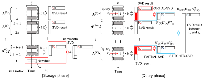
Figure 2. Overview of Zoom-SVD. In the storage phase, Zoom-SVD stores the SVD results for length-$b$ blocks of multiple time series data, updates the SVD result of the most recent block of a newly arrived data, and discards previously arrived data. In the query phase, Zoom-SVD computes the SVD result in a given time range $[t_{s},t_{e}]$ based on the small SVD results. The query phase exploits Partial-SVD (Section 3.3.1) and Stitched-SVD (Section 3.3.2) modules to process the time range query.

2.2. Incremental SVD

Incremental SVD dynamically calculates the SVD result of a matrix with newly arrived data rows. Suppose that we have the SVD result $\mathbf{U}_{t}$, $\mathbf{\Sigma}_{t}$, and $\mathbf{V}^{T}_{t}$ of a data matrix $\mathbf{A}_{t}\in\mathbb{R}^{n\times c}$ at time $t$. When an $m\times c$ matrix $\mathbf{A}_{t+1}$ arrives at time $t+1$, the purpose of incremental SVD is to efficiently obtain the SVD result of $\begin{bmatrix}\mathbf{A}_{t}~{};~{}\mathbf{A}_{t+1}\end{bmatrix}$ based on the previous result $\mathbf{U}_{t}$, $\mathbf{\Sigma}_{t}$, and $\mathbf{V}^{T}_{t}$. Note that $\begin{bmatrix}\mathbf{X}~{};~{}\mathbf{Y}\end{bmatrix}$ denotes the vertical concatenation of two matrices $\mathbf{X}$ and $\mathbf{Y}$. Incremental SVD is used to analyze patterns in time series data (Sarwar et al., 2002), and several efficient methods for incremental SVD were proposed (Brand, 2003; Ross et al., 2008). This incremental SVD technique is exploited in our method to incrementally compress and store the data (see Algorithm 1 in Section 3.2).

2.3. Problem Definition

We formally define the time range query problem as follows:

Problem 1.

(Time Range Query on Multiple Time Series)

• Given: a time range $[t_{s},t_{e}]$, and multiple time series data represented by a matrix $\mathbf{A}\in\mathbb{R}^{t\times c}$ where $t$ is the length of the time dimension, and $c$ is the number of the time series,

• Find: the SVD result of the sub-matrix of $\mathbf{A}$ in the time range quickly, without storing all of $\mathbf{A}$. The SVD result includes $\mathbf{U}\in\mathbb{R}^{(t_{e}-t_{s}+1)\times k}$, $\mathbf{\Sigma}\in\mathbb{R}^{k\times k}$, and $\mathbf{V}\in\mathbb{R}^{c\times k}$ where $k$ is the rank of the sub-matrix.

Applying the standard SVD or incremental SVD for the time range query is impractical for the following reasons. Standard SVD needs to extract the sub-matrix corresponding to the time range before performing decomposition. Iwen et al. (Iwen and Ong, 2016) proposed a hierarchical and distributed approach for computing $\mathbf{\Sigma}$ and $\mathbf{V}$ except for $\mathbf{U}$ of a whole matrix $\mathbf{A}$. Zadeh et al. (Zadeh et al., 2016) introduce Tall and Skinny SVD which obtains $\mathbf{\Sigma}$ and $\mathbf{V}$ by computing eigen-decomposition of $\mathbf{{A}^{T}A}$, and then computes $\mathbf{U}$ using $\mathbf{\Sigma}$, $\mathbf{V}$, and $\mathbf{A}$. Halko et al. (Halko et al., 2011) propose Randomized SVD which computes SVD of $\mathbf{A}$ using randomized approximation techniques. However, such methods are inefficient because they need to compute SVDs from scratch for multiple overlapping queries. Furthermore, those methods need to keep the entire time series data $\mathbf{A}$, which is practically infeasible in many streaming applications. Incremental SVD considers updates only on newly added data, and thus cannot perform SVD on a specific time range.

To address these limitations, we propose an efficient method for the time range query in Section 3.

3. Proposed Method

We propose Zoom-SVD, a fast and space-efficient method for extracting key patterns from multiple time series data in an arbitrary time range. We first give an overview of Zoom-SVD in Section 3.1. We describe details of Zoom-SVD in Sections 3.2 and 3.3. Finally, we analyze Zoom-SVD’s time and space complexities in Section 3.4.

3.1. Overview

Zoom-SVD efficiently extracts key patterns from multiple time series data in an arbitrary time range using SVD. The main challenges for the time range query problem (Problem 1) are as follows:

1. Minimize the space cost. The amount of multiple time series data increases over time. How can we reduce the space while supporting time range queries?

2. Minimize the time cost. How can we quickly compute SVD of multiple time series data in an arbitrary time range?

We address the above challenges with the following ideas:

1. Compress multiple time series data (Section 3.2). Zoom-SVD compresses the raw data using incremental SVD, and discards the raw data in the storage phase.

2. Avoid reconstructing the original data from the SVD results computed in the storage phase (Sections 3.3.1 and 3.3.2). We propose Partial-SVD and Stitched-SVD to compute SVD without reconstructing the original data corresponding to the query time range.

3. Optimize the computational time of Stitched-SVD (Section 3.3.2). We optimize the performance of Stitched-SVD by reducing numerical computations using a block matrix structure.

Zoom-SVD comprises two phases: storage phase and query phase. In the storage phase (Algorithm 1), Zoom-SVD stores the SVD results corresponding to length-$b$ blocks in the time series data in order to support time range queries as shown in Figure 2. When a new data arrives, Zoom-SVD incrementally updates the SVD result with the newly arrived data, block by block. In the query phase (Algorithms 2), Zoom-SVD returns the SVD result for a given time range $[t_{s},t_{e}]$. The query phase utilizes our proposed Partial-SVD and Stitched-SVD modules to process the time range query. Partial SVD (Algorithm 3) manipulates the SVD result containing $t_{s}$ (or $t_{e}$) to match the query time range as shown in Figure 2. Stitched-SVD (Algorithms 2) efficiently computes the SVD result between $t_{s}$ and $t_{e}$ by stitching the SVD results for blocks in the time range.

3.2. Storage Phase of Zoom-SVD

Given multiple time series stream $\mathbf{A}$, the objective of the storage phase is to incrementally compress the input data and discard the original input data $\mathbf{A}$ to achieve space efficiency. A naive incremental SVD would update one large SVD result when the data are newly added. However, this approach is impractical because the processing cost for the newly added data increases over time. Also, the naive incremental SVD does not support a time range query quickly in the query phase because it manipulates the large SVD result stored for the total time regardless of the query time range.

The storage phase of Zoom-SVD (Algorithm 1) is designed to efficiently process newly added data and quickly support time range queries. Given multiple time series data $\mathbf{A}$, the storage phase of Zoom-SVD (Algorithm 1) incrementally compresses the input data block by block using incremental SVD, and discards the original input data $\mathbf{A}$ to reduce space cost. Assume the multiple time series data are represented by a matrix $\mathbf{A}\in\mathbb{R}^{t\times c}$ where $t$ is time length, and $c$ is the number of time series (e.g., sensors). We conceptually divide the matrix $\mathbf{A}$ into length-$b$ blocks represented by $\mathbf{A}^{(i)}\in\mathbb{R}^{b\times c}$ as shown in Figure 2. We then store the low-rank approximation result of each block matrix $\mathbf{A}^{(i)}$, where we exploit an incremental SVD method in the process. We formally define the block matrix $\mathbf{A}^{(i)}$ in Definition 1.

Definition 0 (Block matrix $\mathbf{A}^{(i)}$).

Suppose a multivariate time series is $\mathbf{A}={\begin{bmatrix}\mathbf{a}_{1};\mathbf{a}_{2};\cdots;\mathbf{a}_{t}\end{bmatrix}}$ where $\mathbf{a}_{j}\in\mathbb{R}^{1\times c}$ is the $j$-th row vector of $\mathbf{A}$, and $[;]$ denotes the vertical concatenation of vectors. The $i$-th block matrix $\mathbf{A}^{(i)}$ is then represented as follows:

$$\mathbf{A}^{(i)}\equiv{\begin{bmatrix}\mathbf{a}_{b\times i+1};\mathbf{a}_{b\times i+2};\cdots;\mathbf{a}_{b\times i+b}\end{bmatrix}}$$

where $b$ is a block size. In addition, $\mathbf{A}^{(i)}_{t-1}$ denotes the $i$-th block matrix at time $t-1$ where $i$ indicates the index of the most recent block as shown in Figure 2. Note that the number of rows in $\mathbf{A}^{(i)}_{t-1}$ is less than or equal to $b$. $\Box$

The computed SVD result $\mathbf{U}_{(i)}$, $\mathbf{\Sigma}_{(i)}$, and $\mathbf{V}_{(i)}$ of each block matrix $\mathbf{A}^{(i)}$ are stored as follows.

Definition 0 (Sets of SVD results $\mathcal{U}$, $\mathcal{S}$, and $\mathcal{V}$).

The sets $\mathcal{U}$, $\mathcal{S}$, and $\mathcal{V}$ store the SVD results $\mathbf{U}_{(i)}$, $\mathbf{\Sigma}_{(i)}$, and $\mathbf{V}_{(i)}$ for all $i$, respectively. $\Box$

Note that the original time series data are discarded, and we store only the SVD results which occupy less space than the original data. The SVD results for block matrices are used in the query phase (Algorithm 2). Now we are ready to describe the details of the storage phase.

Algorithm 1 Storage phase of Zoom-SVD

0:  multiple time series data $\mathbf{A}$

0:  set $\mathcal{U}$ of left singular vector matrix $\mathbf{U}_{(i)}$, set $\mathcal{S}$ of singular value matrix $\mathbf{\Sigma}_{(i)}$, and set $\mathcal{V}$ of right singular vector matrix $\mathbf{V}_{(i)}$

0:  block size $b$

1:  Initialize: $\mathbf{U}_{(0,1)}$, $\mathbf{\Sigma}_{(0,1)}$, and $\mathbf{V}_{(0,1)}$ $\leftarrow$ SVD result of $\mathbf{a}_{1}$, block index $i\leftarrow 0$, and time index $t\leftarrow 2$

2:  while $\mathbf{a}_{t}$ is newly arriving do

3:     if $\mathbf{U}_{(i,t-1)}$, $\mathbf{\Sigma}_{(i,t-1)}$, $\mathbf{V}_{(i,t-1)}$ do not exist then

4:        $\mathbf{U}_{(i,t)}$, $\mathbf{\Sigma}_{(i,t)}$, $\mathbf{V}_{(i,t)}$ $\leftarrow$ SVD result of $\mathbf{a}_{t}$

5:     else

6:        $\mathbf{U}_{(i,t)}$, $\mathbf{\Sigma}_{(i,t)}$, $\mathbf{V}_{(i,t)}$ $\leftarrow$ Incremental-SVD ($\mathbf{U}_{(i,t-1)}$, $\mathbf{\Sigma}_{(i,t-1)}$, $\mathbf{V}_{(i,t-1)}$, $\mathbf{a}_{t}$)

7:     end if

8:     if the number of rows of $\mathbf{U}_{(i,t)}$ is equal to $b$ then

9:        $\mathcal{U}\leftarrow\mathcal{U}\cup\{\mathbf{U}_{(i,t)}\}$, $\mathcal{S}\leftarrow\mathcal{S}\cup\{\mathbf{\Sigma}_{(i,t)}\}$, $\mathcal{V}\leftarrow\mathcal{V}\cup\{\mathbf{V}_{(i,t)}\}$

10:        $i\leftarrow i+1$

11:     end if

12:     $t\leftarrow t+1$

13:  end while

The storage phase (Algorithm 1) compresses the multiple time series data block by block using incremental SVD to support time range queries. When new multiple time series data $\mathbf{a}_{t}\in\mathbb{R}^{1\times c}$ are given at time $t$ (line 2), we generate the new SVD result of $\mathbf{a}_{t}$ for the next block matrix $\mathbf{A}^{(i)}_{t}$ if the SVD result are stored in $\mathcal{U}$, $\mathcal{S}$, and $\mathcal{V}$ at time $t-1$ (lines 3 and  4). If not, we have the SVD result $\mathbf{U}_{(i,t-1)}$, $\mathbf{\Sigma}_{(i,t-1)}$, and $\mathbf{V}_{(i,t-1)}$ of the most recent block matrix $\mathbf{A}^{(i)}_{t-1}$ which is the $i$-th block matrix at time $t-1$. Assume that we have the SVD result $\mathbf{U}_{(i,t-1)}$, $\mathbf{\Sigma}_{(i,t-1)}$, and $\mathbf{V}_{(i,t-1)}$ of $\mathbf{A}^{(i)}_{t-1}$ (i.e., the block matrix from time $t-b+1$ to $t-1$ as seen in Figure 2). We then update the SVD result into $\mathbf{U}_{(i,t)}$, $\mathbf{\Sigma}_{(i,t)}$, and $\mathbf{V}_{(i,t)}$ for the new data $\mathbf{a}_{t}$ using an incremental SVD method (line 6). If the number of rows of $\mathbf{U}_{(i,t)}$ is $b$, we put the SVD result $\mathbf{U}_{(i,t)}$, $\mathbf{\Sigma}_{(i,t)}$, and $\mathbf{V}_{(i,t)}$ into $\mathcal{U}$, $\mathcal{S}$, and $\mathcal{V}$, respectively (lines 8$\sim$11). Equations (2) and (3) represent the details of how to update the SVD result of $\mathbf{A}^{(i)}_{t-1}$ for the new incoming data $\mathbf{a}_{t}$, when $\mathbf{A}^{(i)}_{t-1}$ contains $b-1$ rows. $\mathbf{A}^{(i)}_{t}$ is represented by $\mathbf{a}_{t}$ and the SVD result of $\mathbf{A}^{(i)}_{t-1}$ in Equation (2):

(2) $$\footnotesize\begin{split}\mathbf{A}^{(i)}_{t}=\begin{bmatrix}\mathbf{A}^{(i)}_{t-1}\\ \mathbf{a}_{t}\end{bmatrix}&\simeq\begin{bmatrix}\mathbf{U}_{(i,t-1)}\mathbf{\Sigma}_{(i,t-1)}\mathbf{V}^{\text{T}}_{(i,t-1)}\\ \mathbf{a}_{t}\end{bmatrix}\\ &=\begin{bmatrix}\mathbf{U}_{(i,t-1)}&\mathbf{O}_{(b-1)\times 1}\\ \mathbf{O}_{1\times k_{t-1}}&\mathbf{I}_{1\times 1}\end{bmatrix}\begin{bmatrix}\mathbf{\Sigma}_{(i,t-1)}\mathbf{V}^{\text{T}}_{(i,t-1)}\\ \mathbf{a}_{t}\end{bmatrix}\end{split}$$

where $\mathbf{O}_{x\times y}$ is an $x\times y$ zero matrix, and $\mathbf{I}_{x\times x}$ is an $x\times x$ identity matrix. We then perform SVD to decompose $\begin{bmatrix}\mathbf{\Sigma}_{(i,t-1)}\mathbf{V}^{\text{T}}_{(i,t-1)}\\ \mathbf{a}_{t}\end{bmatrix}$ $\in\mathbb{R}^{(k_{t-1}+1)\times c}$ into $\mathbf{\tilde{U}}\mathbf{\tilde{\Sigma}}\mathbf{\tilde{V}}^{\text{T}}$:

(3) $$\footnotesize\begin{split}&\begin{bmatrix}\mathbf{U}_{(i,t-1)}&\mathbf{O}_{(b-1)\times 1}\\ \mathbf{O}_{1\times k_{t-1}}&\mathbf{I}_{1\times 1}\end{bmatrix}\begin{bmatrix}\mathbf{\Sigma}_{(i,t-1)}\mathbf{V}^{\text{T}}_{(i,t-1)}\\ \mathbf{a}_{t}\end{bmatrix}\\ &=\begin{bmatrix}\mathbf{U}_{(i,t-1)}&\mathbf{O}_{(b-1)\times 1}\\ \mathbf{O}_{1\times k_{t-1}}&\mathbf{I}_{1\times 1}\end{bmatrix}\mathbf{\tilde{U}}\mathbf{\tilde{\Sigma}}\mathbf{\tilde{V}}^{\text{T}}\triangleq\mathbf{U}_{(i,t)}\mathbf{\Sigma}_{(i,t)}\mathbf{V}^{\text{T}}_{(i,t)}\end{split}$$

where $\mathbf{U}_{(i,t)}=$ $\begin{bmatrix}\mathbf{U}_{(i,t-1)}&\mathbf{O}_{(b-1)\times 1}\\ \mathbf{O}_{1\times k_{t-1}}&\mathbf{I}_{1\times 1}\end{bmatrix}$ $\mathbf{\tilde{U}}$, $\mathbf{\Sigma}_{(i,t)}=\mathbf{\tilde{\Sigma}}$, and $\mathbf{V}^{\text{T}}_{(i,t)}=\mathbf{\tilde{V}}^{\text{T}}$. Note that $\mathbf{U}_{(i,t)}$ is a column orthogonal matrix since it is the product of two orthogonal matrices. $\mathbf{V}_{(i,t)}$ is also column orthogonal, and $\mathbf{\Sigma}_{(i,t)}$ is a diagonal matrix whose diagonal entries are sorted in the descending order. Hence, $\mathbf{U}_{(i,t)}$, $\mathbf{\Sigma}_{(i,t)}$, and $\mathbf{V}_{(i,t)}$ are considered as the SVD result of $\mathbf{A}^{(i)}_{t}$ by the definition of SVD (Trefethen and Bau III, 1997). The time index $t$ can be omitted as in $\mathbf{U}_{(i)}$, $\mathbf{\Sigma}_{(i)}$, $\mathbf{V}_{(i)}$, and $\mathbf{A}^{(i)}$, as described in Definitions 1 and 2, if the number of rows of $\mathbf{U}_{(i,t)}$ is $b$.

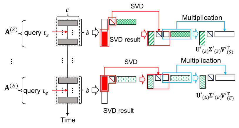
Figure 3. Example of Partial-SVD. Given a time range query $[t_{s},t_{e}]$, we remove rows of $\mathbf{U}_{(S)}$ and $\mathbf{U}_{(E)}$ which are out of the query time range. Partial-SVD exploits SVD on the filtered matrices for left singular vector matrices and singular value matrices within the query time range (red-colored boxes). Then Partial-SVD computes right singular vector matrices of the output SVD results by multiplying relevant matrices (blue-colored boxes).

3.3. Query Phase of Zoom-SVD

Given the starting point $t_{s}$ and the ending point $t_{e}$ of a time range query, the goal of the query phase of Zoom-SVD is to obtain the SVD result from $t_{s}$ to $t_{e}$. A naive approach would reconstruct the time series data from the SVD results of the block matrices ranged between $t_{s}$ and $t_{e}$, and perform SVD on the reconstructed data in the range. However, this approach requires heavy computations especially for a long time range query, and thus is not appropriate for serving time range queries quickly.

We propose two sub-modules, Partial-SVD and Stitched-SVD, which are used in the query phase of our proposed method (Algorithm 2) to efficiently process time range queries by avoiding reconstruction of the raw data. Let $S$ be the index of the block matrix including $t_{s}$, and $E$ be the index of the block matrix including $t_{e}$. Partial-SVD (Algorithm 3) adjusts the time range of the SVD results for $\mathbf{A}^{(S)}$ and $\mathbf{A}^{(E)}$ as seen in the red-colored boxes of Figure 3 (line 1 of Algorithm 2). Stitched-SVD combines the SVD results of Partial-SVD and those of block matrices from $\mathbf{A}^{(S+1)}$ to $\mathbf{A}^{(E-1)}$ (lines  2 to  5 in Algorithm 2). We describe the details of Partial-SVD and Stitched-SVD in Sections 3.3.1 and 3.3.2, respectively.

Algorithm 2 Query phase of Zoom-SVD

0:  sets $\mathcal{U}$, $\mathcal{S}$, and $\mathcal{V}$ of block SVD results, starting point $t_{s}$, and ending point $t_{e}$

0:  SVD result $\mathbf{U}_{(S:E)}$, $\mathbf{\Sigma}_{(S:E)}$, and $\mathbf{V}_{(S:E)}$ in $[t_{s},t_{e}]$

1:  $\mathbf{U}_{(S)}^{\prime}$, $\mathbf{\Sigma}_{(S)}^{\prime}$, $\mathbf{V}_{(S)}^{\prime}$, $\mathbf{U}_{(E)}^{\prime}$, $\mathbf{\Sigma}_{(E)}^{\prime}$, and $\mathbf{V}_{(E)}^{\prime}$ $\leftarrow$ Partial-SVD ($t_{s}$, $t_{e}$, $\mathcal{U},\mathcal{S},\mathcal{V}$)

2:  $\mathbf{\Sigma}\mathbf{V}^{\text{T}}\leftarrow[\mathbf{\Sigma^{\prime}}_{(S)}\mathbf{V^{\prime}}^{\text{T}}_{(S)};\mathbf{\Sigma}_{(S+1)}\mathbf{V}^{\text{T}}_{(S+1)};\cdots;\mathbf{\Sigma^{\prime}}_{(E)}\mathbf{V^{\prime}}^{\text{T}}_{(E)}]$

3:  $\mathbf{U}_{r},\mathbf{\Sigma}_{r},\mathbf{V}^{\text{T}}_{r}\leftarrow$ low-rank approximation of $\mathbf{\Sigma}\mathbf{V}^{\text{T}}$ using SVD

4:  $\mathbf{V}_{(S:E)}\leftarrow\mathbf{V}_{r}$ and $\mathbf{\Sigma}_{(S:E)}\leftarrow\mathbf{\Sigma}_{r}$

5:  $\mathbf{U}_{(S:E)}$ $\leftarrow$ $[\mathbf{U}_{(S)}^{\prime}\mathbf{U}^{\prime}_{r(S)}~{};~{}\mathbf{U}_{(S+1)}\mathbf{U}_{r(S+1)}~{};~{}\cdots~{};~{}\mathbf{U}_{(E)}^{\prime}\mathbf{U}^{\prime}_{r(E)}]$

6:  return  $\mathbf{U}_{(S:E)}$, $\mathbf{\Sigma}_{(S:E)}$, and $\mathbf{V}_{(S:E)}$

3.3.1. Partial-SVD

This module manipulates the SVD results of block matrices $\mathbf{A}^{(S)}$ and $\mathbf{A}^{(E)}$ to return the SVD results in a given time range $[t_{s},t_{e}]$. As seen in Figure 2, $\mathbf{A}^{(S)}$ may contain the time range before $t_{s}$, and $\mathbf{A}^{(E)}$ may include the time range after $t_{e}$. Note that those time ranges are out of the time range of the given query; thus, our goal for this module is to extract SVD results from $\mathbf{A}^{(S)}$ and $\mathbf{A}^{(E)}$ according to the time range query without reconstructing raw data. Figure 3 depicts the operation of Partial-SVD. For the block matrix $\mathbf{A}^{(S)}$ and its SVD $\mathbf{U}_{(S)}\mathbf{\Sigma}_{(S)}\mathbf{V}_{(S)}$, Partial-SVD first eliminates rows of left singular vector matrix $\mathbf{U}_{(S)}$ which are out of the query time range. After that, Partial-SVD multiplies the remaining left singular vector matrix $\mathbf{X}_{s}\mathbf{U}_{(S)}$ with the singular value matrix $\mathbf{\Sigma}_{(S)}$, and performs SVD $\mathbf{\tilde{U}}_{(S)}\mathbf{\tilde{\Sigma}}_{(S)}\mathbf{\tilde{V}}^{\text{T}}_{(S)}\leftarrow\mathbf{X}_{s}\mathbf{U}_{(S)}\mathbf{\Sigma}_{(S)}$ of the resulting matrix. The resulting singular vector matrix $\mathbf{\tilde{U}}_{(S)}$ and the singular value matrix $\mathbf{\tilde{\Sigma}}_{(S)}$ constitute the output of Partial-SVD. The remaining right singular vector matrix output of Partial-SVD is computed by multiplying the right singular vector matrix $\mathbf{\tilde{V}}^{\text{T}}_{(S)}$ with $\mathbf{V}^{\text{T}}_{(S)}$. Similar operations are performed for the block matrix $\mathbf{A}^{(E)}$ and its SVD $\mathbf{U}_{(E)}\mathbf{\Sigma}_{(E)}\mathbf{V}_{(E)}$.

Now, we describe the details of this module (Algorithm 3). We first introduce elimination matrices which are used in Partial-SVD to adjust the time range.

Definition 0 (Elimination matrices).

Suppose $r_{S}$ is the number of rows to be eliminated in $\mathbf{A}^{(S)}$ according to $t_{s}$. Then $b_{S}=b-r_{S}$ is the number of remaining rows in $\mathbf{A}^{(S)}$. Similarly, let $r_{E}$ be the number of rows to be eliminated in $\mathbf{A}^{(E)}$ according to $t_{e}$; then $b_{E}=b-r_{E}$ is the number of remaining rows in $\mathbf{A}^{(E)}$. The elimination matrices $\mathbf{X}_{s}$ and $\mathbf{X}_{e}$ for $\mathbf{A}^{(S)}$ and $\mathbf{A}^{(E)}$ are defined as follows:

(4) $$\mathbf{X}_{s}=\begin{bmatrix}\mathbf{O}_{b_{S}\times r_{S}}&\mathbf{I}_{b_{S}\times b_{S}}\end{bmatrix}\mathbf{X}_{e}=\begin{bmatrix}\mathbf{I}_{b_{E}\times b_{E}}&\mathbf{O}_{b_{E}\times r_{E}}\end{bmatrix}$$

$\Box$

Algorithm 3 Partial-SVD

0:  starting point $t_{s}$, ending point $t_{e}$, and sets $\mathcal{U}$, $\mathcal{S}$, and $\mathcal{V}$ of SVD results

0:  SVD results $\mathbf{U}_{(S)}^{\prime}$, $\mathbf{\Sigma}_{(S)}^{\prime}$, $\mathbf{V}_{(S)}^{\prime}$, $\mathbf{U}_{(E)}^{\prime}$, $\mathbf{\Sigma}_{(E)}^{\prime}$, and $\mathbf{V}_{(E)}^{\prime}$ of $\mathbf{A}^{(S)}$ and $\mathbf{A}^{(E)}$ within the time range

1:  $S\leftarrow t_{s}/b$ and $E\leftarrow t_{e}/b$

2:  $b_{S}\leftarrow b-t_{s}\%b$ and $b_{E}\leftarrow t_{e}\%b$ (%: the modulus operator)

3:  construct $\mathbf{X}_{s}$ and $\mathbf{X}_{e}$ based on $b_{S}$ and $b_{E}$ as in Equation (4)

4:  $\mathbf{\tilde{U}}_{(S)}$, $\mathbf{\tilde{\Sigma}}_{(S)}$, $\mathbf{\tilde{V}}^{\text{T}}_{(S)}$ $\leftarrow$ low-rank approximation of $\mathbf{X}_{s}\mathbf{U}_{(S)}\mathbf{\Sigma}_{(S)}$ using SVD

5:  $\mathbf{U}_{(S)}^{\prime}\leftarrow\mathbf{\tilde{U}}_{(S)}$, $\mathbf{\Sigma}_{(S)}^{\prime}\leftarrow\mathbf{\tilde{\Sigma}}_{(S)}$, and $\mathbf{V^{\prime}}^{\text{T}}_{(S)}\leftarrow\mathbf{\tilde{V}}^{\text{T}}_{(S)}\mathbf{V}^{\text{T}}_{(S)}$

6:  $\mathbf{\tilde{U}}_{(E)}$, $\mathbf{\tilde{\Sigma}}_{(E)}$, $\mathbf{\tilde{V}}^{\text{T}}_{(E)}$ $\leftarrow$ low-rank approximation of $\mathbf{X}_{e}\mathbf{U}_{(E)}\mathbf{\Sigma}_{(E)}$ using SVD

7:  $\mathbf{U}_{(E)}^{\prime}\leftarrow\mathbf{\tilde{U}}_{(E)}$, $\mathbf{\Sigma}_{(E)}^{\prime}\leftarrow\mathbf{\tilde{\Sigma}}_{(E)}$, and $\mathbf{V^{\prime}}^{\text{T}}_{(E)}\leftarrow\mathbf{\tilde{V}}^{\text{T}}_{(E)}\mathbf{V}^{\text{T}}_{(E)}$

8:  return  $\mathbf{U}_{(S)}^{\prime}$, $\mathbf{\Sigma}_{(S)}^{\prime}$, $\mathbf{V}_{(S)}^{\prime}$, $\mathbf{U}_{(E)}^{\prime}$, $\mathbf{\Sigma}_{(E)}^{\prime}$, and $\mathbf{V}_{(E)}^{\prime}$

The matrices $\mathbf{A}^{(S)}$ and $\mathbf{A}^{(E)}$ are multiplied to the elimination matrices, and the time ranges of the resulting matrices $\mathbf{X}_{s}\mathbf{A}^{(S)}$ and $\mathbf{X}_{e}\mathbf{A}^{(E)}$ are within the query time range $[t_{s},t_{e}]$. Partial-SVD constructs those elimination matrices based on $b_{S}$ and $b_{E}$ (line 3 of Algorithm 3). The filtered block matrix $\mathbf{X}_{s}\mathbf{A}^{(S)}$ is given by

(5) $$\mathbf{X}_{s}\mathbf{A}^{(S)}\simeq\mathbf{X}_{s}(\mathbf{U}_{(S)}\mathbf{\Sigma}_{(S)}\mathbf{V}^{\text{T}}_{(S)})=(\mathbf{X}_{s}\mathbf{U}_{(S)}\mathbf{\Sigma}_{(S)})\mathbf{V}^{\text{T}}_{(S)}$$

where $\mathbf{A}^{(S)}\simeq\mathbf{U}_{(S)}\mathbf{\Sigma}_{(S)}\mathbf{V}^{\text{T}}_{(S)}$ was computed at the storage phase.

Partial-SVD decomposes $\mathbf{X}_{s}\mathbf{U}_{(S)}\mathbf{\Sigma}_{(S)}$ into $\mathbf{\tilde{U}}_{(S)}\mathbf{\tilde{\Sigma}}_{(S)}\mathbf{\tilde{V}}^{\text{T}}_{(S)}$ via SVD and low-rank approximation with threshold $\xi$ since $\mathbf{X}_{s}\mathbf{U}_{(S)}$ is not a column orthogonal matrix, and $\mathbf{X}_{s}\mathbf{U}_{(S)}\mathbf{\Sigma}_{(S)}\mathbf{V}^{\text{T}}_{(S)}$ is not a form of the SVD result; then, Equation (5) is written as follows:

(6) $$\small(\mathbf{X}_{s}\mathbf{U}_{(S)}\mathbf{\Sigma}_{(S)})\mathbf{V}^{\text{T}}_{(S)}\!\simeq\!\mathbf{\tilde{U}}_{(S)}\mathbf{\tilde{\Sigma}}_{(S)}(\mathbf{\tilde{V}}_{(S)}\mathbf{V}_{(S)})^{\text{T}}\!=\!\mathbf{U}_{(S)}^{\prime}\mathbf{\Sigma}_{(S)}^{\prime}\mathbf{V^{\prime}}^{\text{T}}_{(S)}$$

where $\mathbf{U}_{(S)}^{\prime}=\mathbf{\tilde{U}}_{(S)}$, $\mathbf{\Sigma}_{(S)}^{\prime}=\mathbf{\tilde{\Sigma}}_{(S)}$, and $\mathbf{V^{\prime}}^{\text{T}}_{(S)}=\mathbf{\tilde{V}}^{\text{T}}_{(S)}\mathbf{V}^{\text{T}}_{(S)}$. In line 4, Partial-SVD performs SVD on $\mathbf{X}_{s}\mathbf{U}_{(S)}\mathbf{\Sigma}_{(S)}$, and in line 5 it computes $\mathbf{V^{\prime}}^{\text{T}}_{(S)}=\mathbf{\tilde{V}}^{\text{T}}_{(S)}\mathbf{V}^{\text{T}}_{(S)}$. Partial-SVD similarly computes the SVD result of $\mathbf{X}_{e}\mathbf{A}^{(E)}$ in lines 6$\sim$7 of Algorithm 3.

3.3.2. Stitched-SVD

This module combines the Partial-SVD of $\mathbf{A}^{(S)}$ and $\mathbf{A}^{(E)}$, and the stored SVD results of blocks matrices $\mathbf{A}^{(S+1)},\mathbf{A}^{(S+1)},\cdots,\mathbf{A}^{(E-1)}$ in the query time range $[t_{s},t_{e}]$ to return the final SVD result corresponding to the query range as shown in Figure 2. A naive approach is to reconstruct the data blocks using the stored SVD results and perform SVD on the reconstructed data of the given query time range. However, this approach cannot provide fast query speed for a long time range due to heavy computations induced by the reconstruction and the following SVD. The goal of Stitched-SVD is to efficiently stitch the SVD results in the query time range by avoiding reconstruction and minimizing the numerical computation of matrix multiplication.

Specifically, Stitched-SVD stitches several consecutive block SVD results together to compute the SVD corresponding to the query time range: is.e., it combines the SVD result $\mathbf{U}_{(i)}$, $\mathbf{\Sigma}_{(i)}$, and $\mathbf{V}_{(i)}$ of the $i$th block matrix $\mathbf{A}^{(i)}$, for $i=S..E$, to compute the SVD $\mathbf{U}_{(S:E)}$, $\mathbf{\Sigma}_{(S:E)}$, and $\mathbf{V}_{(S:E)}$. The main idea is 1) to carefully decouple the matrices $\mathbf{U}_{(i)}$ from $\mathbf{\Sigma}_{(i)}$$\mathbf{V}_{(i)}$, 2) construct a stacked matrix containing $\mathbf{\Sigma}_{(i)}$$\mathbf{V}_{(i)}$ for $i=S..E$, 3) perform SVD on the stacked matrix to get the singular value matrix and the right singular vector matrix of the final SVD result, and 4) carefully combine $\mathbf{U}_{(i)}$ with the left singular matrix of SVD of the stacked matrix to get the left singular vector matrix of the final SVD result.

Lines 2 to 5 of Algorithm 2 present how stitched SVD matrices are computed. First, we construct $\footnotesize\mathbf{\Sigma}\mathbf{V}^{\text{T}}$ based on the block matrix structure where $\footnotesize\mathbf{\Sigma}\mathbf{V}^{\text{T}}$ is equal to $\footnotesize{\begin{bmatrix}\mathbf{\Sigma^{\prime}}_{(S)}\mathbf{V^{\prime}}^{\text{T}}_{(S)}~{};~{}\mathbf{\Sigma}_{(S+1)}\mathbf{V}^{\text{T}}_{(S+1)}~{};~{}\cdots~{};~{}\mathbf{\Sigma^{\prime}}_{(E)}\mathbf{V^{\prime}}^{\text{T}}_{(E)}\end{bmatrix}}^{T}$. After organizing the block matrix structure of $\footnotesize\mathbf{\Sigma}\mathbf{V}^{\text{T}}$, we define block diagonal matrix $diag(S:E)$ as follows.

Definition 0 (Block diagonal matrix).

Suppose $\mathbf{U}_{(S)}^{\prime}$ and $\mathbf{U}_{(E)}^{\prime}$ are the left singular vector matrices produced by Partial-SVD. Let $\mathbf{U}_{(S+1)}$, $\mathbf{U}_{(S+2)}$, $\cdots$, $\mathbf{U}_{(E-1)}$ be the left singular vector matrices in $\mathcal{U}$. The block diagonal matrix $diag(S:E)$ is defined as follows:

$$\footnotesize diag(S:E)=\begin{bmatrix}\mathbf{U}_{(S)}^{\prime}&\mathbf{O}&\cdots&\mathbf{O}\\ \mathbf{O}&\mathbf{U}_{(S+1)}&&\vdots\\ \vdots&&\ddots&\vdots\\ \mathbf{O}&\cdots&\cdots&\mathbf{U}_{(E)}^{\prime}\\ \end{bmatrix}$$

$\Box$

Then, the matrix corresponding to the time range query $[t_{s},t_{e}]$ is represented as follows:

(7) $$\footnotesize\begin{split}\mathbf{A}^{(S:E)}&=\begin{bmatrix}\mathbf{X}_{s}\mathbf{A}^{(S)}\\ \mathbf{A}^{(S+1)}\\ \cdots\\ \mathbf{X}_{e}\mathbf{A}^{(E)}\end{bmatrix}\simeq\begin{bmatrix}\mathbf{U}_{(S)}^{\prime}\mathbf{\Sigma}_{(S)}^{\prime}\mathbf{V^{\prime}}^{\text{T}}_{(S)}\\ \mathbf{U}_{(S+1)}\mathbf{\Sigma}_{(S+1)}\mathbf{V}^{\text{T}}_{(S+1)}\\ \cdots\\ \mathbf{U}_{(E)}^{\prime}\mathbf{\Sigma}_{(E)}^{\prime}\mathbf{V^{\prime}}^{\text{T}}_{(E)}\\ \end{bmatrix}=diag(S:E)\mathbf{\Sigma}\mathbf{V}^{\text{T}}\end{split}$$

where $\mathbf{X}_{s}$ and $\mathbf{X}_{e}$ are elimination matrices of Partial-SVD, and $\mathbf{\Sigma}\mathbf{V}^{\text{T}}$ is equal to $\footnotesize{\begin{bmatrix}\mathbf{\Sigma^{\prime}}_{(S)}\mathbf{V^{\prime}}^{\text{T}}_{(S)}~{};~{}\mathbf{\Sigma}_{(S+1)}\mathbf{V}^{\text{T}}_{(S+1)}~{};~{}\cdots~{};~{}\mathbf{\Sigma^{\prime}}_{(E)}\mathbf{V^{\prime}}^{\text{T}}_{(E)}\end{bmatrix}}^{T}$. As we apply SVD and low-rank approximation to $\mathbf{\Sigma}\mathbf{V}^{\text{T}}$, Equation (7) becomes as follows:

(8) $$\begin{split}diag(S:E)\mathbf{\Sigma}\mathbf{V}^{\text{T}}&\simeq diag(S:E)\mathbf{U}_{r}\mathbf{\Sigma}_{r}\mathbf{V}^{\text{T}}_{r}\\ &=\mathbf{U}_{(S:E)}\mathbf{\Sigma}_{(S:E)}\mathbf{V}^{\text{T}}_{(S:E)}\end{split}$$

where $\mathbf{\Sigma}\mathbf{V}^{\text{T}}\simeq\mathbf{U}_{r}\mathbf{\Sigma}_{r}\mathbf{V}^{\text{T}}_{r}$ is computed by low-rank approximation and SVD, $\mathbf{U}_{(S:E)}=diag(S:E)\mathbf{U}_{r}$, $\mathbf{\Sigma}_{(S:E)}=\mathbf{\Sigma}_{r}$, and $\mathbf{V}_{(S:E)}=\mathbf{V}_{r}$. To avoid matrix multiplication between $\mathbf{U}_{r}$ and zero sub-matrices of $diag(S:E)$, we split $\mathbf{U}_{r}$ block by block as follows:

$$\footnotesize\mathbf{U}_{r}={\begin{bmatrix}\mathbf{U}^{\prime}_{r(S)}~{};~{}\mathbf{U}_{r(S+1)}~{};~{}\cdots~{};~{}\mathbf{U}^{\prime}_{r(E)}\end{bmatrix}}^{T}$$

where $\mathbf{U}^{\prime}_{r(S)}$ and $\mathbf{U}^{\prime}_{r(E)}$ correspond to $\mathbf{U}_{(S)}^{\prime}$ and $\mathbf{U}_{(E)}^{\prime}$, respectively, and $\mathbf{U}_{r(i)}$ correspond to $\mathbf{U}_{(i)}$ for $S+1\leq i\leq E-1$. Then $\mathbf{U}_{(S:E)}=diag(S:E)\mathbf{U}_{r}$ of Equation (8) is computed as follows:

(9) $$\begin{split}&\mathbf{U}_{(S:E)}=diag(S:E)\mathbf{U}_{r}\\ &={\begin{bmatrix}\mathbf{U}_{(S)}^{\prime}\mathbf{U}^{\prime}_{r(S)}~{};~{}\mathbf{U}_{(S+1)}\mathbf{U}_{r(S+1)}~{};~{}\cdots~{};~{}\mathbf{U}_{(E)}^{\prime}\mathbf{U}^{\prime}_{r(E)}\end{bmatrix}}^{T}\end{split}$$

The column orthogonality of $\mathbf{U}_{(S:E)}=diag(S:E)\mathbf{U}_{r}$ is established as it is the product of two column orthogonal matrices; also, $\mathbf{V}_{(S:E)}=\mathbf{V}_{r}$ is column orthogonal. Note that we perform Partial-SVD to satisfy column orthogonal condition before performing Stitched-SVD.

3.4. Theoretical Analysis

We theoretically analyze our proposed method Zoom-SVD in terms of time and memory cost. Note that a collection of multiple time series data $\mathbf{A}$ is a dense matrix, and the time complexity to compute SVD of $\mathbf{A}\in\mathbb{R}^{t\times c}$ is $O(min(t^{2}c,tc^{2}))$.

Time Complexity. We analyze the time complexities of the storage and the query phases in Theorems 5 and 6, respectively.

Theorem 5.

When a vector $\mathbf{a}_{t}\in\mathbb{R}^{1\times c}$ is given at time $t$, the computation cost of storage phase in Zoom-SVD is $O(k^{2}(b+c))$, where $k$ is the number of singular values.

Proof.

Performing SVD of ${\begin{bmatrix}\mathbf{\Sigma}_{(i,t-1)}\mathbf{V}^{\text{T}}_{(i,t-1)}~{};~{}\mathbf{a}_{t}\end{bmatrix}}$ takes $O(min(c^{2}$ $(1+k_{t-1}),c(1+k_{t-1})^{2})$, and multiplication of $\begin{bmatrix}\mathbf{U}_{(i,t-1)}&\mathbf{O}\\ \mathbf{O}&\mathbf{I}\end{bmatrix}$ and $\mathbf{\tilde{U}}$ takes $O(b(k_{t-1}+1)k_{t})$ since the row length of $\begin{bmatrix}\mathbf{U}_{(i,t-1)}&\mathbf{O}\\ \mathbf{O}&\mathbf{I}\end{bmatrix}$ is always smaller than or equal to the block size $b$. Assume $k_{t-1}$ and $k_{t}$ are equal to $k$. The total computational cost of storage phase in Zoom-SVD is O($min(c^{2}k,ck^{2})$+ $bk^{2}$). We simply express the computational cost of storing the incoming data at each time tick as $O(k^{2}(b+c))$ since the number $c$ of columns is generally greater than $k$. ∎

In Theorem 5, the computation of storing the incoming data at each time tick takes constant time since $b$ and $c$ are constants and $k$ is smaller than $c$.

Theorem 6.

Given a time range query $[t_{s},t_{e}]$, the time cost of query phase (Algorithm 2) is $O((t_{e}-t_{s})k(k+\frac{c^{2}}{b})+{k^{2}}(b+c))$.

Proof.

It takes $O((b-r_{S}+c)k^{\prime 2}_{(S)}+(b-r_{E}+c)k^{\prime 2}_{(E)})$ to compute Partial-SVD where $k^{\prime}_{(S)}$ and $k^{\prime}_{(E)}$ are the number of singular values computed by Partial-SVD (line 1 in Algorithm 2). The computational time to perform SVD of $\footnotesize{\begin{bmatrix}\mathbf{\Sigma^{\prime}}_{(S)}\mathbf{V^{\prime}}^{\text{T}}_{(S)}~{};~{}\mathbf{\Sigma}_{(S+1)}\mathbf{V}^{\text{T}}_{(S+1)}~{};~{}\cdots~{};~{}\mathbf{\Sigma^{\prime}}_{(E)}\mathbf{V^{\prime}}^{\text{T}}_{(E)}\end{bmatrix}}$ depends on $O(min(c^{2}(k^{\prime}_{(S)}+k^{\prime}_{(E)}+{\sum_{i=S+1}^{E-1}k_{(i)}})$, $c(k^{\prime}_{(S)}+k^{\prime}_{(E)}+{\sum_{i=S+1}^{E-1}k_{(i)}})^{2})$ in Stitched-SVD since horizontal and vertical length of the matrix are $c$ and $(k^{\prime}_{(S)}+k^{\prime}_{(E)}+{\sum_{i=S+1}^{E-1}k_{(i)}})$, respectively (lines 2$\sim$ 4 in Algorithm 2). Also, the computational time of block matrix multiplication for $\mathbf{U}_{(S:E)}$ (line 5 in Algorithm 2) takes O($k_{(S:E)}$
($(b-r_{S})k^{\prime}_{(S)}$$+(b-r_{E})k^{\prime}_{(E)}+b{\sum_{i=S+1}^{E-1}k_{(i)}}$)) where $k_{(S:E)}$ is the number of singular values with respect to the SVD result of a given time range $[t_{s},t_{e}]$. Let all $k_{(i)}$’s be $k$ in query phase, $k^{\prime}_{(S)}+k^{\prime}_{(E)}+{\sum_{i=S+1}^{E-1}k_{(i)}}$ be larger than $c$; also, replace $b-r_{i}$ with block size $b$ since $b$ is always greater than $b-r_{i}$. Then, the computational time of Partial-SVD and Stitched-SVD takes $O(k^{2}(b+c))$ and $O((t_{e}-t_{s})k(k+\frac{c^{2}}{b}))$, respectively. We can simply express the computational cost of Zoom-SVD as $O((t_{e}-t_{s})k(k+\frac{c^{2}}{b})+{k^{2}}(b+c))$. ∎

Theorem 6 implies that the computational time of Zoom-SVD in query phase linearly depends on the time range $(t_{e}-t_{s})$.

Space Complexity. We analyze the space complexity of the storage phase in Theorem 7.

Theorem 7.

Space complexity of Zoom-SVD for storing data is $O(tk(1+\frac{k}{b}+\frac{c}{b}))$ where $t$ is the total time length, and $k$ is the number of singular values.

Proof.

At time $t$, we have $\lfloor\frac{t}{b}\rfloor$ SVD results where $\mathbf{U}_{(i)}\in\mathbb{R}^{b_{i}\times k_{(i)}}$, $\mathbf{\Sigma}_{(i)}\in\mathbb{R}^{k_{(i)}\times k_{(i)}}$, and $\mathbf{V}_{(i)}\in\mathbb{R}^{k_{(i)}\times c}$. Therefore, the number of elements in every matrix we have is $O(\sum_{i=1}^{\lfloor\frac{t}{b}\rfloor}k_{(i)}(b+k_{(i)}+c))$. Assuming $k_{(i)}$ is equal to $k$, we briefly express the space cost of Zoom-SVD as $O(tk(1+\frac{k}{b}+\frac{c}{b}))$. ∎

The space cost linearly depends on $t$ and $k$, but $k$ is much smaller than the number $c$ of time series. Therefore, Zoom-SVD efficiently compresses incoming data using space linear to time length with low coefficient.

4. Experiment

Table 2. Description of real-world multiple time series datasets. Each dataset is a matrix in $\mathbb{R}^{t\times c}$ where $t$ corresponds to total length (time), and $c$ corresponds to the number of time series.

Dataset	Total length ($t$)	Attribute ($c$)
Activity	382,000	41
Gas	4,107,000	16
London	350,000	10

We aim to answer the following questions to evaluate the performance of our method Zoom-SVD from experiments.

• Q1. Time cost (Section 4.2). How quickly does Zoom-SVD process time range queries compared to other methods?

• Q2. Space cost (Section 4.3). How much memory space does Zoom-SVD require for compressed blocks?

• Q3. Time-Space-Accuracy Trade-off (Section 4.4). What are the tradeoffs between query time, space, and accuracy by Zoom-SVD compared to other baselines?

• Q4. Parameter (Section 4.5). How does the block size $b$ in Algorithm 1 affect the performance of Zoom-SVD in terms of time and space?

4.1. Experiment Settings

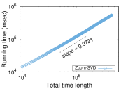
(a) Running time of Zoom-SVD’s storage phase in Activity dataset

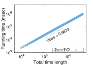
(b) Running time of Zoom-SVD’s storage phase in Gas dataset

Figure 4. Running time of Zoom-SVD’s storage phase on Activity and Gas datasets. The results show that the time to update all data is linear to the total time length $t$. The reason is that Zoom-SVD incrementally reads a new input vector, and computes the SVD of the block matrix in a constant time. The pattern on London dataset is similar to the above results.

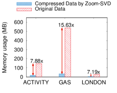
Figure 5. Space savings by Zoom-SVD. Zoom-SVD requires $7.88\times$, $15.63\times$, and $7.19\times$ less space than the original data require for Activity, Gas sensor, and London, respectively.

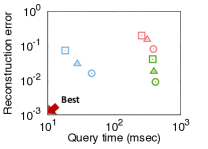
(a) Query time vs Error in Activity

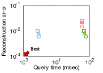
(b) Query time vs Error in Gas

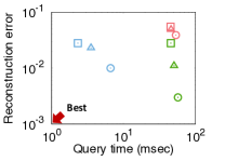
(c) Query time vs Error in London

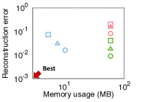
(d) Memory usage vs Error in Activity

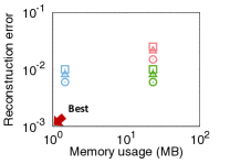
(e) Memory usage vs Error in Gas

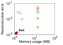
(f) Memory usage vs Error in London

Figure 6. The trade-off between query time, space, and MSE rate on three real-world datasets. The first column shows the results on the Activity dataset. The second and third columns show the results on the Gas and the London datasets. The colors represent the methods, and the shapes distinguish the threshold $\xi$. The bottom-left region indicates the better performance. On all the real-world datasets, Zoom-SVD has the best performance.

Methods. We compare Zoom-SVD with Randomized SVD (Halko et al., 2011), Tall and Skinny SVD (Zadeh et al., 2016), and basic SVD of JBLAS library. All these methods are implemented using JAVA, and we use JBLAS, an open source JAVA basic linear algebra package, to support matrix operations.

Dataset. We use multiple time series datasets (Reiss and Stricker, 2012; Fonollosa et al., 2015) described in Table 2. Activity dataset contains data with timestamps, and 41 measured values such as heartbeat, and inertial measurement units (IMU) data installed in the hands, chest, and ankle. Gas dataset consists of timestamps, and measurement of 16 chemical sensors having 4 different types. Activity and Gas datasets are obtained from UCI repository (Dheeru and Karra Taniskidou, 2017). London dataset consists of timestamps, and attributes related to London air quality such as nitric oxide, temperature, and so on.

Parameters. For all experiments except the ones in Section 4.5, we set the block size $b$ to $1000$ in the storage phase. We evaluate the effects of the block size $b$ in Section 4.5. We set the rank $k$ using Equation (1) with $\xi=0.98$ in the storage phase.

4.2. Time Cost

We examine the time costs of the storage and the query phases of our proposed method Zoom-SVD.

Storage phase (Algorithm 1). We measure the running time of the storage phase for multiple time series data varying the time length. As shown in Figure 4, the running time of Zoom-SVD’s storage phase is linearly proportional to the time length over all datasets. The reason is that the storage phase processes the time series data row by row, and the time cost of processing a row is constant as discussed in Theorem 5; thus, the total time cost mainly depends on the time length.

Query phase (Algorithm 2). We evaluate the performance of the query phase in terms of running time. We compare Zoom-SVD to other SVD based methods discussed in Section 2, and measure the query time varying the length of the query range. The starting and the ending points of the query are arbitrarily chosen, and we increase the length of the query range from $10^{4}$ to $3.2\times 10^{5}$. As shown in Figure 1, Zoom-SVD is up to $9.6\times$ faster than the second best competitor Randomized SVD on Activity dataset. Also, Zoom-SVD shows up to $15\times$ and $12\times$ faster query speed than Randomized SVD on Gas sensor and London datasets, respectively.

4.3. Space Cost

We evaluate the compression performance of Zoom-SVD. In the storage phase, we store the SVD results of multiple time series data with block size $b=10^{3}$ using low-rank approximation with threshold $\xi=0.98$ in Equation (1). We measure the compression ratio for storing the original data and the block compressed data (i.e., the SVD results) by our method. Figure 5 shows the compression performance for storing time series data. Zoom-SVD requires up to $7.88\times$, $15.63\times$, and $7.19\times$ less space than the original data require for Activity, Gas, and London, respectively.

4.4. Trade-off between Accuracy and Efficiency

We evaluate the trade-off of Zoom-SVD between accuracy, time, and space compared to other methods. We measure the time and the space usage by setting the length of time range query to $1.8\times 10^{5}$. The accuracy of each method is measured by the reconstruction error $\frac{\lVert\mathbf{X}_{(t_{s}:t_{e})}-\hat{\mathbf{X}}_{(t_{s}:t_{e})}\rVert^{2}_{F}}{\lVert\mathbf{X}_{(t_{s}:t_{e})}\rVert^{2}_{F}}$ where $\hat{\mathbf{X}}_{(t_{s}:t_{e})}$ is the reconstructed data (i.e., $\hat{\mathbf{X}}_{(t_{s}:t_{e})}=\mathbf{U}_{(S,E)}\mathbf{\Sigma}_{(S,E)}\mathbf{V}_{(S,E)}^{T}$), and $\mathbf{X}_{(t_{s}:t_{e})}$ is the original input data in a query time range $[t_{s},t_{e}]$. We use the values $0.95$, $0.98$, and $0.99$ for the threshold $\xi$ in the low-rank approximation of each method to investigate the effect of $\xi$ on the trade-off performance. Figure 6 demonstrates the experimental results on the trade-off of SVD based methods including Zoom-SVD. Figures 6(a), 6(b), and 6(c) present the trade-off of Zoom-SVD between query time and reconstruction error is better than those of other methods over all the datasets. Also, Zoom-SVD shows a better trade-off between space and reconstruction error than its competitors as shown in Figures 6(d), 6(e), and 6(f). These results indicate that Zoom-SVD handles time range queries more efficiently with smaller error and space than other SVD based methods.

4.5. Parameter Sensitivity

We examine the effects of the block size $b$ in terms of query time, and space cost. When the block size $b$ grows from $10$ to $10^{5}$, we measure the query time and the memory usage in query phase by setting the query time range $t_{e}-t_{s}+1$ to $10^{3}$, $10^{4}$, and $10^{5}$ in Algorithm 2. In Figure 7, the query time and memory usage show trade-off characteristics. The query time and the space usage for Activity dataset decrease until the block size reaches $10^{2}\sim 10^{3}$, and then increase afterwards when the block size $b$ exceeds $10^{3}$. Note that Zoom-SVD consists of Partial-SVD and Stitched-SVD modules in the query phase. In Figure 7(a), the query time is dominated by the computation time of the Stitched-SVD when the block size $b$ is relatively small. The reason is that the computation time of Partial-SVD decreases as the block size $b$ decreases, while that of Stitched-SVD increases linearly with the number of blocks which is inversely proportional to the block size. On the other hand, the query time highly depends on the computation time of Partial-SVD when the block size is relatively large. In Figure 7(b), space cost is high when $b$ is small because the number of stored singular vector matrices for blocks increases. On the other hand, space cost is also high when $b$ is large because the number $k$ of singular values increases as the block size $b$ increases, and then the size of left singular vector matrices $\mathbf{U}_{(i)}$ increases. Therefore, we set the block size $b$ to $10^{3}$ which is a near-optimum value according to the experimental results. The sensitivities of Zoom-SVD on the block size $b$ in other datasets show similar patterns.

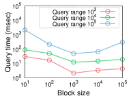
(a) Query time vs. block size

(b) Space cost vs. block size

Figure 7. The effect of the block size $b$ in terms of the query time and the memory usage in Activity dataset. When the block size $b$ grows from $10$ to $10^{5}$, the query time and the memory usage decrease until the block size is $10^{3}$, and then increase continuously after block size exceeds $10^{3}$.

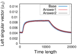
(a) First left singular vector

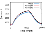
(b) Sensor 1

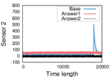
(c) Sensor 2

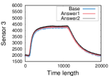
(d) Sensor 3

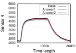
(e) Sensor 4

Figure 8. First left singular vectors of the base and two time ranges having the similar patterns to that of the base. Answer1 and Answer2 are the past time ranges we found using Zoom-SVD by sliding a window. The time range of Answer1 is $[1589294,1609293]$, and that of Answer2 is $[2736794,2756793]$. In (a), the three left singular vectors have the same pattern. In (b, c, d, e), each sensor shows similar measurements for the three ranges in general. Note that Zoom-SVD discovers a potential anomaly: (c) shows an abnormal spike of Base around $17,960$, which deviates vastly from the measurements of the past ranges.

5. Case Study

In this section, we present the analysis result of Gas sensor dataset using Zoom-SVD. For a given time range, Zoom-SVD searches past time ranges for similar patterns to that of the given time range.

Data description. Gas sensor dataset consists of 16 chemical sensors exposed to gas mixtures which contain ethylene and carbon monoxide (CO) with air. There are four different types of sensors: TGS2600, TGS2602, TGS2610, and TGS2620 (four sensors per one type). The sensors are placed in a 60ml measurement chamber. The electrical conductivities of the sensors are measured at every 0.01 seconds, and the total time length is 12 hours.

Finding similar time ranges. Our goal is to find past time ranges whose patterns are similar to that of a given time range query which we call as the ‘base’. Suppose a time range $[t_{s},t_{e}]$ is given. First, we compute SVD of data in the range using Zoom-SVD. Next, we continuously compute SVDs of previous time ranges using Zoom-SVD by sliding a window of size $t_{e}-t_{s}+1$. Note that we use the fixed window size for efficiency. We then compare $\mathbf{u_{1}}$ of the base with $\mathbf{\overline{u}_{1}}$ of previous time ranges, where $\mathbf{u_{1}}$ is the first column of left singular vector matrix $\mathbf{U}$ of the base, and $\mathbf{\overline{u}_{1}}$ is the first column of $\mathbf{\overline{U}}$ of a previous time range. Experimental setting is as follows:

• The base time range is $[4033294,4053293]$ which is randomly chosen, and thus the size of sliding window (time length) is $20,000$. The sliding period is $500$.

• We compute the cosine similarity $\frac{\mathbf{u_{1}}\cdot\mathbf{\overline{u}_{1}}}{\lVert\mathbf{u_{1}}\rVert\lVert\mathbf{\overline{u}_{1}}\rVert}$ to compare the patterns, and then find the two most similar time ranges.

Figure 8 shows the first singular vectors of the given time range (denoted by ’Base’) and two previous time ranges (denoted by ’Answer1’ and ’Answer2’) with similar patterns we found, and sensor data corresponding to each time range. In Figure 8(a), Zoom-SVD successfully finds the similar patterns, and each sensor has the same tendency w.r.t. the three time ranges. We also discover a potential anomaly. In Figure 8(c), note an abnormal spike of Base at the time around $17,960$, which deviates significantly from the measurements of the two previous time ranges.

6. Related Work

In this section, we discuss related works on incremental time series analysis and incremental SVD.

It is important to analyze on-line time series data efficiently. There are several ideas based on linear modeling, including Kalman Filters (KF), linear dynamical systems (LDS) and the variants (Jain et al., 2004; Li et al., 2010, 2009), time warping (Toyoda et al., 2013), and correlation-based methods (Mueen et al., 2010; Sakurai et al., 2005; Zhu and Shasha, 2002; Keogh et al., 2001). Among them, incremental SVD efficiently tracks the SVD of dynamic time series data where new data rows are incrementally attached to the current data. Incremental SVD has been used for updating SVD results when new terms or documents are added to a document-term matrix (Deerwester et al., 1990), and has been adopted to build an incremental movie recommender system (Sarwar et al., 2002; Brand, 2003). Brand (Brand, 2002) developed an incremental SVD method for incomplete data which contain missing values. Papadimitriou et al. (Papadimitriou et al., 2005) proposed SPIRIT which incrementally updates hidden factors in multiple time series, and exploited SPIRIT to predict future signals and interpolate missing values in sensor streams. Ross et al. (Ross et al., 2008) proposed an incremental PCA for visual tracking applications. Papadimitriou et al. (Papadimitriou and Yu, 2006) introduced an incremental method to capture optimal recurring patterns indicating the main trends in time series data.

The methods above have limitations in applying to time range query problem. Conventional methods such as Discrete Fourier Transformation (Mueen et al., 2010), data compression (Reeves et al., 2009; Gandhi et al., 2009), and time series clustering (Paparrizos and Gravano, 2015) require the whole time series data, or additional data to seek hidden patterns for a specific time range, thereby incurring high memory and time complexity. On the other hand, our proposed Zoom-SVD efficiently serves time range queries with small memory and low time complexity.

7. Conclusions

We propose Zoom-SVD, a novel algorithm for finding key patterns in an arbitrary time range from multiple time series data. Zoom-SVD efficiently serves time range queries by compressing multiple time series data, and reducing computation costs by carefully stitching compressed SVD results. Consequently, Zoom-SVD provides fast query time and small memory usage. We provide theoretical analysis on the time and space complexities of Zoom-SVD. Experiments show that Zoom-SVD requires up to $15.66\times$ less space, and runs up to $15\times$ faster than existing methods. Also, we show a real-world case study of Zoom-SVD in searching past time ranges for similar patterns as that of a query time range. Future research includes extending the method for multiple distributed streams.

- (1)
- Brand (2002) Matthew Brand. 2002. Incremental singular value decomposition of uncertain data with missing values. ECCV (2002), 707–720.
- Brand (2003) Matthew Brand. 2003. Fast online svd revisions for lightweight recommender systems. In SDM. 37–46.
- Deerwester et al. (1990) Scott Deerwester, Susan T Dumais, George W Furnas, Thomas K Landauer, and Richard Harshman. 1990. Indexing by latent semantic analysis. Journal of the American society for information science 41, 6 (1990), 391.
- Dheeru and Karra Taniskidou (2017) Dua Dheeru and Efi Karra Taniskidou. 2017. UCI Machine Learning Repository. (2017). http://archive.ics.uci.edu/ml
- Fonollosa et al. (2015) Jordi Fonollosa, Sadique Sheik, Ramón Huerta, and Santiago Marco. 2015. Reservoir computing compensates slow response of chemosensor arrays exposed to fast varying gas concentrations in continuous monitoring. Sensors and Actuators B: Chemical 215 (2015), 618–629.
- Gandhi et al. (2009) Sorabh Gandhi, Suman Nath, Subhash Suri, and Jie Liu. 2009. Gamps: Compressing multi sensor data by grouping and amplitude scaling. In SIGMOD. ACM, 771–784.
- Halko et al. (2011) Nathan Halko, Per-Gunnar Martinsson, and Joel A. Tropp. 2011. Finding Structure with Randomness: Probabilistic Algorithms for Constructing Approximate Matrix Decompositions. SIAM Rev. 53, 2 (2011), 217–288.
- Iwen and Ong (2016) M. A. Iwen and B. W. Ong. 2016. A Distributed and Incremental SVD Algorithm for Agglomerative Data Analysis on Large Networks. SIAM J. Matrix Analysis Applications 37, 4 (2016), 1699–1718.
- Jain et al. (2004) Ankur Jain, Edward Y Chang, and Yuan-Fang Wang. 2004. Adaptive stream resource management using kalman filters. In SIGMOD. ACM, 11–22.
- Jeon et al. (2016a) ByungSoo Jeon, Inah Jeon, Lee Sael, and U. Kang. 2016a. SCouT: Scalable coupled matrix-tensor factorization - algorithm and discoveries. In ICDE. 811–822.
- Jeon et al. (2016b) Inah Jeon, Evangelos E. Papalexakis, Christos Faloutsos, Lee Sael, and U. Kang. 2016b. Mining billion-scale tensors: algorithms and discoveries. VLDB J. 25, 4 (2016), 519–544.
- Jeon et al. (2015) Inah Jeon, Evangelos E. Papalexakis, U. Kang, and Christos Faloutsos. 2015. HaTen2: Billion-scale Tensor Decompositions. In ICDE. 1047–1058.
- Jolliffe (2002) Ian Jolliffe. 2002. Principal component analysis. Wiley Online Library.
- Kang et al. (2011) U. Kang, Brendan Meeder, and Christos Faloutsos. 2011. Spectral Analysis for Billion-Scale Graphs: Discoveries and Implementation. In PAKDD. 13–25.
- Kang et al. (2014) U Kang, B. Meeder, E. Papalexakis, and C. Faloutsos. 2014. HEigen: Spectral Analysis for Billion-Scale Graphs. Knowledge and Data Engineering, IEEE Transactions on 26, 2 (February 2014), 350–362. https://doi.org/10.1109/TKDE.2012.244
- Kang et al. (2012) U. Kang, Hanghang Tong, and Jimeng Sun. 2012. Fast Random Walk Graph Kernel. In SDM. 828–838.
- Keogh et al. (2001) Eamonn J. Keogh, Kaushik Chakrabarti, Sharad Mehrotra, and Michael J. Pazzani. 2001. Locally Adaptive Dimensionality Reduction for Indexing Large Time Series Databases. In SIGMOD. 151–162.
- Koren et al. (2009) Yehuda Koren, Robert Bell, and Chris Volinsky. 2009. Matrix factorization techniques for recommender systems. Computer 42, 8 (2009), 30–37.
- Li et al. (2009) Lei Li, James McCann, Nancy S Pollard, and Christos Faloutsos. 2009. Dynammo: Mining and summarization of coevolving sequences with missing values. In KDD. ACM, 507–516.
- Li et al. (2010) Lei Li, B Aditya Prakash, and Christos Faloutsos. 2010. Parsimonious linear fingerprinting for time series. PVLDB 3, 1-2 (2010), 385–396.
- Mueen et al. (2010) Abdullah Mueen, Suman Nath, and Jie Liu. 2010. Fast approximate correlation for massive time-series data. In SIGMOD. ACM, 171–182.
- Oh et al. (2018) Sejoon Oh, Namyong Park, Lee Sael, and U. Kang. 2018. Scalable Tucker Factorization for Sparse Tensors - Algorithms and Discoveries. In ICDE. 1120–1131.
- Osiński et al. (2004) Stanisław Osiński, Jerzy Stefanowski, and Dawid Weiss. 2004. Lingo: Search results clustering algorithm based on singular value decomposition. In Intelligent information processing and web mining. Springer, 359–368.
- Papadimitriou et al. (2005) Spiros Papadimitriou, Jimeng Sun, and Christos Faloutsos. 2005. Streaming Pattern Discovery in Multiple Time-Series. In VLDB. 697–708.
- Papadimitriou and Yu (2006) Spiros Papadimitriou and Philip S. Yu. 2006. Optimal multi-scale patterns in time series streams. In SIGMOD. 647–658.
- Paparrizos and Gravano (2015) John Paparrizos and Luis Gravano. 2015. k-shape: Efficient and accurate clustering of time series. In SIGMOD. ACM, 1855–1870.
- Park et al. (2017) Haekyu Park, Jinhong Jung, and U. Kang. 2017. A comparative study of matrix factorization and random walk with restart in recommender systems. In BigData. 756–765.
- Park et al. (2016) Namyong Park, ByungSoo Jeon, Jungwoo Lee, and U. Kang. 2016. BIGtensor: Mining Billion-Scale Tensor Made Easy. In CIKM. 2457–2460.
- Ravi Kanth et al. (1998) KV Ravi Kanth, Divyakant Agrawal, and Ambuj Singh. 1998. Dimensionality reduction for similarity searching in dynamic databases. In SIGMOD, Vol. 27. ACM, 166–176.
- Reeves et al. (2009) Galen Reeves, Jie Liu, Suman Nath, and Feng Zhao. 2009. Managing massive time series streams with multi-scale compressed trickles. PVLDB 2, 1 (2009), 97–108.
- Reiss and Stricker (2012) Attila Reiss and Didier Stricker. 2012. Introducing a New Benchmarked Dataset for Activity Monitoring. In ISWC. 108–109.
- Ross et al. (2008) David A Ross, Jongwoo Lim, Ruei-Sung Lin, and Ming-Hsuan Yang. 2008. Incremental learning for robust visual tracking. International journal of computer vision 77, 1 (2008), 125–141.
- Sael et al. (2015) Lee Sael, Inah Jeon, and U Kang. 2015. Scalable Tensor Mining. Big Data Research 2, 2 (2015), 82 – 86. https://doi.org/10.1016/j.bdr.2015.01.004 Visions on Big Data.
- Sakurai et al. (2005) Yasushi Sakurai, Spiros Papadimitriou, and Christos Faloutsos. 2005. Braid: Stream mining through group lag correlations. In SIGMOD. ACM, 599–610.
- Sarwar et al. (2002) Badrul Sarwar, George Karypis, Joseph Konstan, and John Riedl. 2002. Incremental singular value decomposition algorithms for highly scalable recommender systems. In ICIS. 27–28.
- Simek et al. (2004) Krzysztof Simek, Krzysztof Fujarewicz, Andrzej Świerniak, Marek Kimmel, Barbara Jarzab, Małgorzata Wiench, and Joanna Rzeszowska. 2004. Using SVD and SVM methods for selection, classification, clustering and modeling of DNA microarray data. Engineering Applications of Artificial Intelligence 17, 4 (2004), 417–427.
- Spiegel et al. (2011) Stephan Spiegel, Julia Gaebler, Andreas Lommatzsch, Ernesto De Luca, and Sahin Albayrak. 2011. Pattern recognition and classification for multivariate time series. In Sensor-KDD. ACM, 34–42.
- Tong et al. (2006) Hanghang Tong, Christos Faloutsos, and Jia-yu Pan. 2006. Fast Random Walk with Restart and Its Applications. In ICDM. 613–622.
- Toyoda et al. (2013) Machiko Toyoda, Yasushi Sakurai, and Yoshiharu Ishikawa. 2013. Pattern discovery in data streams under the time warping distance. VLDBJ 22, 3 (2013), 295–318.
- Trefethen and Bau III (1997) Lloyd N Trefethen and David Bau III. 1997. Numerical linear algebra. Vol. 50. Siam.
- Wall et al. (2003) Michael E Wall, Andreas Rechtsteiner, and Luis M Rocha. 2003. Singular value decomposition and principal component analysis. In A practical approach to microarray data analysis. Springer, 91–109.
- Zadeh et al. (2016) Reza Bosagh Zadeh, Xiangrui Meng, Alexander Ulanov, Burak Yavuz, Li Pu, Shivaram Venkataraman, Evan R. Sparks, Aaron Staple, and Matei Zaharia. 2016. Matrix Computations and Optimization in Apache Spark. In KDD. 31–38.
- Zhu and Shasha (2002) Yunyue Zhu and Dennis Shasha. 2002. Statstream: Statistical monitoring of thousands of data streams in real time. In VLDB. VLDB Endowment, 358–369.