Gaussian processes with multidimensional distribution inputs via optimal transport and Hilbertian embedding

Abstract

In this work, we investigate Gaussian Processes indexed by multidimensional distributions. While directly constructing radial positive definite kernels based on the Wasserstein distance has been proven to be possible in the unidimensional case, such constructions do not extend well to the multidimensional case as we illustrate here. To tackle the problem of defining positive definite kernels between multivariate distributions based on optimal transport, we appeal instead to Hilbert space embeddings relying on optimal transport maps to a reference distribution, that we suggest to take as a Wasserstein barycenter. We characterize in turn radial positive definite kernels on Hilbert spaces, and show that the covariance parameters of virtually all parametric families of covariance functions are microergodic in the case of (infinite- dimensional) Hilbert spaces. We also investigate statistical properties of our suggested positive definite kernels on multidimensional distributions, with a focus on consistency when a population Wasserstein barycenter is replaced by an empirical barycenter and additional explicit results in the special case of Gaussian distributions. Finally, we study the Gaussian process methodology based on our suggested positive definite kernels in regression problems with multidimensional distribution inputs, on simulation data stemming both from synthetic examples and from a mechanical engineering test case.

1 Introduction

Gaussian process models are widely used in fields such as geostatistics, computer experiments and machine learning Rasmussen and Williams (2006), Santner et al. (2003). In a nutshell, Gaussian process modelling consists in assuming for an unknown function of interest to be one realisation of a Gaussian process, or equivalently of a Gaussian random field indexed by the source space of the objective function, and is often cast as part of the Bayesian arsenal for non-parametric estimation in function spaces. For instance, in computer experiments, the input points of the function are simulation input parameters and the output values are quantities of interest obtained from simulation responses. Furthermore, there has been a huge amount of literature dealing with the use of Gaussian Processes in Machine Learning over the last decade. We refer for instance to Rasmussen (2004), Schölkopf and Smola (2002) or Cristianini and Shawe-Taylor (2000) and references therein.

Gaussian process models heavily rely on the specification of a covariance function, or “kernel”, that characterises linear dependencies between values of the process at different observation points. In fact, the kernel, which can be seen as a similarity measure between locations in index space, also induces a (pseudo-)metric on the index space often referred to as the “canonical metric associated with the kernel” via the variogram function of geostatisticians. A natural question for a given kernel is how those inherently associated notions of similarity/dissimilarity interplay with prescribed metrics on the index space. In Euclidean space, one often speaks of radial kernel for those covariance functions that are explicitly depending on the Euclidean distance between points. Radial kernels with respect to other metrics have also be investigated, see e.g. kernels writing as functions of the $\ell^{1}$ distance in multivariate Euclidean spaces Wendland (2004).

In this paper we consider Gaussian processes indexed by distributions supported on $\mathbb{R}^{p}$, and we investigate ways to build positive definite kernels based on the Wasserstein distance. Distributional inputs can occur in a number of practical situations and exploring admissible kernels for using Gaussian Process and related methods in this context is a pressing issue. Situations of that kind include the case of uncertain vector inputs to a vector-to-scalar deterministic function, but also a variety of other settings such as histogram inputs standing for instance for ratings from a panel of experts, compositional data in geosciences, or randomized strategies in a Bayesian game-theoretic framework.

In some situations, distribution-valued inputs may arise as a convenient way to describe complex objects and media, e.g. a number of physical simulations require maps or parameter fields as inputs, and in some cases it can be beneficial to reparametrize them so as to work with probabiliy distributions. For instance in Ginsbourger et al. (2016), the computer model http://www cast3m.cea.fr is studied, where the input simulation parameter consists of a set of disks located on a unit square $[0,1]^{2}$, modelling a material, for which a stress measure is associated. A Gaussian process model on distributions enables to treat the input sets of disks as measures, and to model the stress values as stemming from a random field indexed by the input distributions.

In this framework, a natural aim is to construct covariance functions for Gaussian processes indexed by such inputs, that is constructing positive definite kernels on sets of probability measures.

The simplest method is perhaps to compare a set of parametric features built from the probability distributions, such as the mean or the higher moments. This approach is limited, as the effect of such parameters does not take the whole distribution into account. Specific positive definite kernels should be designed in order to map distributions into a reproducing kernel Hilbert space in which the whole arsenal of kernel methods can be extended to probability measures. This issue has recently been considered in Muandet et al. (2016) or Kolouri et al. (2015). We aim at basing these kernels on the Wasserstein, or transport-based, distance which was shown to be relevant and insightful for comparing or studying distributions Villani (2009); Chernozhukov et al. (2017); Peyré et al. (2019).

This issue has been studied for the one dimensional case in Bachoc et al. (2018a) or in Trang Bui et al. (2018), using the special expression of the Wasserstein distance in dimension 1. Yet this case uses the property of the optimal coupling with the uniform random variable which is very specific to the one dimensional case. The positive definite kernels provided in the one dimensional case are not positive definite any longer, when they are extended to higher dimensions, as we illustrate numerically in Section 5.

In the general dimension case, in order to build a positive definite kernel from the Wasserstein distance, we associate to each input distribution its optimal transport map to a reference distribution. We then provide positive definite kernels on the Hilbert space corresponding to these optimal transport maps. This results in a positive definite kernel for multidimensional distributions. As a reference distribution, we recommend to take the empirical Fréchet mean (or barycenter) of the distributions. We remark that the notion of Wasserstein barycenters and their use in machine learning and in statistics has been tackled recently in, for instance, Agueh and Carlier (2011), Bigot and Klein (2012), Boissard et al. (2015). Although computational aspects of optimal transports are a difficult issue, substantial work has been conducted to provide feasible algorithms to compute barycenters and optimal transport maps, see for instance Kroshnin et al. (2019),  Uribe et al. (2018), or Peyré et al. (2019) and references therein. Thus our suggested procedure is feasible in practice, as is confirmed by our simulation results on simulated data and on the data from the CASTEM computer model http://www cast3m.cea.fr ; Ginsbourger et al. (2016).

We also characterize all the continuous radial positive definite kernels on Hilbert spaces. This is carried out by showing that they coincide with continuous radial positive definite kernels on Euclidean spaces of arbitrary dimension, and by revisiting existing results for the Euclidean case Wendland (2004). In addition, we show that when considering parametric families of covariance functions for Gaussian processes on infinite dimensional Hilbert spaces, all the covariance parameters are microergodic in general. Microergodicity is an important concept for the asymptotic analysis of Gaussian processes Stein (1999); Zhang (2004); Anderes (2010).

We provide furthermore statistical results related to our positive definite kernel construction. We study the asymptotic closeness of the two kernels obtained by taking the empirical barycenter and the population barycenter as reference distributions. We obtain additional more quantitative results in the special case of Gaussian input distributions. We also discuss stationarity and universality.

In the aforementioned simulations, we compare the Gaussian process regression model obtained from our suggested positive definite kernels with the distribution regression procedure of Poczos et al. (2013). The results show the benefit of our method.

The paper falls into the following parts. In Section 2 we recall some definitions on kernels and on the notion of optimal transport, Wasserstein distance and Wasserstein barycenter of distributions . We also provide our positive definite kernel construction. The analysis of positive definite kernels and Gaussian processes on Hilbert spaces is provided in Section 3. Section 4 is devoted to the statistical results related to our kernel construction. The simulation results are provided in Section 5. Conclusions are discussed in Section 6. The proofs are postponed to the appendix.

2 Construction of positive definite kernels for distributions with Hilbert space embedding and optimal transport

2.1 Background

Gaussian process models are now widely used in fields such as geostatistics, computer experiments or machine learning Rasmussen and Williams (2006), Santner et al. (2003). A Gaussian process model consists in modelling an unknown function as a realisation of a Gaussian process, and hence corresponds to a functional Bayesian framework. For instance, in computer experiments, the input points of the function are simulation parameters and the output values are quantities of interest obtained from the simulations. In this paper we focus on Gaussian processes for which the input parameters are in $\mathcal{P}(\mathbb{R}^{p})$ the set of distributions supported on $\mathbb{R}^{p}$. To study such models, Gaussian Processes must be defined over the set of distributions.

Let us recall that a Gaussian process $(Y_{x})_{x\in E}$ indexed by a set $E$ is entirely characterised by its mean and covariance functions. A covariance function is defined by $(x,y)\in E\times E\to\mathrm{Cov}(Y_{x},Y_{y})$. In general, a function $K:E\times E\mapsto\mathbb{R}$ is actually the covariance of a random process if and only if it is a positive definite kernel, that is for every $x_{1},\cdots,x_{n}\in E$ and $\lambda_{1},\cdots,\lambda_{n}\in\mathbb{R},$

$$\sum_{i,j=1}^{n}\lambda_{i}\lambda_{j}K(x_{i},x_{j})\geq 0.$$ (2.1)

In this case we say that $K$ is a covariance kernel. If the quadratic form (2.1) is always strictly positive when $x_{1},\ldots,x_{n}$ are two-by-two distinct, then we say that $K$ is a strictly positive definite kernel.

We also say that $K$ is a conditionally negative definite kernel if the quadratic form in (2.1) is non-positive when $\sum_{i=1}^{n}\lambda_{i}=0$.

The notions of Wasserstein distance and optimal transport will be central to our construction of positive definite kernels on $\mathcal{P}(\mathbb{R}^{p})$. Let us introduce them now (see also Villani (2009)). Let us consider the set $\mathcal{W}_{2}({\mathbb{R}^{p}})$ of probability measures on $\mathbb{R}^{p}$ with finite moments of order two. For two $\mu,\nu$ in $\mathcal{W}_{2}\left(\mathbb{R}^{p}\right)$ , we denote by $\varPi(\mu,\nu)$ the set of all probability measures $\pi$ over the product set $\mathbb{R}^{p}\times\mathbb{R}^{p}$ with first (resp. second) marginal $\mu$ (resp. $\nu$).

The transportation cost with quadratic cost function, or quadratic transportation cost, between these two measures $\mu$ and $\nu$ is defined as

$$\mathcal{T}_{2}(\mu,\nu)=\inf_{\pi\in\varPi(\mu,\nu)}\int\left\|x-y\right\|^{2}d\pi(x,y).$$ (2.2)

In the above display and throughout this paper, we let $\|\cdot\|$ be the Euclidean norm on any Euclidean space. This transportation cost allows to endow the set $\mathcal{W}_{2}\left(\mathbb{R}^{p}\right)$ with a metric by defining the quadratic Monge-Kantorovich, or quadratic Wasserstein distance between $\mu$ and $\nu$ as

$$W_{2}(\mu,\nu)=\mathcal{T}_{2}(\mu,\nu)^{1/2}.$$ (2.3)

A probability measure $\pi$ in $\varPi(\mu,\nu)$ realizing the infimum in (2.2) is called an optimal coupling. A random vector $(X_{1},X_{2})$ with distribution $\pi$ in $\varPi(\mu,\nu)$ realizing this infimum is also called an optimal coupling.

Our aim is to base our suggested covariance functions on the notion of optimal transport. Indeed, the Wasserstein distance has been shown to be a very useful tool in statistics and machine learning Peyré et al. (2019); Chernozhukov et al. (2017).

In the one dimensional case, it is actually possible to create covariance functions which values at $\mu,\nu\in\mathcal{W}_{2}(\mathbb{R}^{p})$ are functions of $W_{2}(\mu,\nu)$ Bachoc et al. (2018a). Indeed, in this case, using a covariance based on the Wasserstein distance amounts to using the following well-known optimal coupling (see Villani (2009)). For all $\mu\in\mathcal{P}(\mathbb{R})$ with finite second order moments, let

$$Z_{\mu}:=F^{-1}_{\mu}(U),$$ (2.4)

where $F^{-1}_{\mu}$ is defined as

$$F^{-1}_{\mu}(t)=\inf\{u,F_{\mu}(u)\geq t\},$$

and denotes the quantile function of the distribution $\mu$ and where $U$ is a uniform random variable on $[0,1]$. This coupling, given by $\{Z_{\mu}\}$, can be seen as a non-Gaussian random field indexed by the set of distributions on the real line with finite second order moments. As such, its variogram

$$(\mu,\nu)\mapsto\mathbb{E}(Z_{\mu}-Z_{\nu})^{2}$$ (2.5)

defines a conditionally negative definite kernel, equal to $W_{2}^{2}(\mu,\nu)$ since the coupling $(Z_{\mu})$ is optimal. This kernel can be used to construct families of covariance functions based on the one-dimensional Wasserstein distance, see Bachoc et al. (2018a).

In general dimension, however, there is no indication that functions of the form $(\mu,\nu)\to F\left(W_{2}(\mu,\nu)\right)$, where $F(|\cdot|)$ is a standard covariance function on $\mathbb{R}$, are positive definite kernels. For instance, in Section 5 we provide simulations where the function $(\mu,\nu)\to\exp(-W_{2}(\mu,\nu)^{2})$ fails to be a positive definite kernel in the case $p=2$ (while it is indeed a valid kernel when $p=1$, see Bachoc et al. (2018a)).

To tackle this issue, we will use the notion of Wasserstein barycenters, that we now introduce. When dealing with a collection of distributions $\mu_{1},\dots,\mu_{n}$, we can define a notion of variation of these distributions. For any $\nu\in\mathcal{W}_{2}({\mathbb{R}^{p}})$, set

$${\rm Var}(\nu)=\sum_{i=1}^{n}W_{2}^{2}(\nu,\mu_{i}).$$

Finding the distribution minimizing the variance of the distributions has been tackled when defining the notion of barycenter of distributions with respect to Wasserstein’s distance in the seminal work of Agueh and Carlier (2011). More precisely, given $p\geq 1$, they provide conditions to ensure existence and uniqueness of the barycenter of the probability measures $(\mu_{i})_{1\leq i\leq n}$ with weights $(\lambda_{i})_{1\leq i\leq n}$, i.e. a minimizer of the following criterion

$$\nu\mapsto\sum_{i=1}^{n}\lambda_{i}W_{2}^{2}(\nu,\mu_{i}).$$ (2.6)

In the last years several works have studied the empirical properties of the barycenters and their applications to several fields. We refer for instance to Bigot and Klein (2012); Boissard et al. (2015) and references therein. Hence the Wasserstein barycenter or Fréchet mean of distribution appears to be a meaningful feature to represent the mean variations of a set of distributions.

This notion of Wasserstein barycenter has been recently extended to distributions defined on $\mathcal{W}_{2}(\mathcal{W}_{2}(\mathbb{R}^{p}))$, that is the set of measures on $\mathcal{W}_{2}(\mathbb{R}^{p})$ with finite expected variances. Let $\mathbb{P}$ be a distribution in $\mathcal{W}_{2}(\mathcal{W}_{2}(\mathbb{R}^{p}))$ and consider $\mu_{1},\dots,\mu_{n}$ i.i.d probabilities drawn according to the distribution $\mathbb{P}$. In this framework, the Wasserstein distance between distributions on $\mathcal{W}_{2}(\mathbb{R}^{p})$ is defined, for any $\nu\in\mathcal{W}_{2}(\mathbb{R}^{p})$, as

$$W_{2}^{2}(\mathbb{P},\delta_{\nu})=\int W^{2}_{2}(\nu,\mu)d\mathbb{P}(\mu).$$ (2.7)

If $\widetilde{\mu}$ is a random distribution obeying law $\mathbb{P}$, this corresponds to

$$W^{2}_{2}(\mathbb{P},\delta_{\nu})=\mathbb{E}_{\{\widetilde{\mu}\sim\mathbb{P}\}}W^{2}_{2}(\widetilde{\mu},\nu).$$

Note that we use the same notations for the Wasserstein distances over distributions in $\mathcal{W}_{2}(\mathbb{R}^{p})$ and over distributions on distributions in $\mathcal{W}_{2}(\mathcal{W}_{2}(\mathbb{R}^{p}))$. The space $\mathcal{W}_{2}(\mathcal{W}_{2}(\mathbb{R}^{p}))$ inherits the properties of the space $\mathcal{W}_{2}(\mathbb{R}^{p})$ and is a good choice for considering asymptotic properties of Wasserstein barycenteric sequences.

We define (if it exists) the Wasserstein barycenter of $\mathbb{P}$ as a probability measure $\overline{\mu}$ in $\mathcal{W}_{2}(\mathbb{R}^{p})$ such that

$$\int W^{2}_{2}(\overline{\mu},\mu)d\mathbb{P}(\mu)=\inf\left\{\int W^{2}_{2}(\nu,\mu)d\mathbb{P}(\mu),\>\nu\in\mathcal{W}_{2}(\mathbb{R}^{p})\right\}.$$

First, we point out that the notion of barycenter developed in (2.6) also corresponds to the barycenter of the atomic probability $\mathbb{P}$ on the Wasserstein space, defined by

$$\mathbb{P}=\sum_{i=1}^{n}\lambda_{i}\delta_{\mu_{i}}.$$

We also recall some facts on the Wasserstein barycenter that are used in the rest of the paper. The following theorem from Alvarez-Esteban et al. (2015) guarantees the existence and uniqueness of this barycenter under some assumptions.

Theorem 1 (Existence of a Wasserstein Barycenter).

Let $\mathbb{P}\in\mathcal{W}_{2}(\mathcal{W}_{2}(\mathbb{R}^{p}))$. Assume that every distribution in the support of $\mathbb{P}$ is absolutely continuous with respect to Lebesgue measure on $\mathbb{R}^{p}$. Then there exists a unique distribution $\overline{\mu}\in\mathcal{P}$ defined as

$$\overline{\mu}={\rm arg}\min_{\nu\in\mathcal{W}_{2}(\mathbb{R}^{p})}\left\{\int W^{2}_{2}(\nu,\mu)d\mathbb{P}(\mu)\right\}.$$ (2.8)

Using the expression (2.7), we can see that Theorem 1 can be reformulated as stating the existence of the metric projection of $\mathbb{P}$ onto the subset of $\mathcal{W}_{2}(\mathcal{W}_{2}(\mathbb{R}^{p}))$ composed of Dirac measures.

Consider a sample of i.i.d random distributions $\mu_{i},\>i=1,\dots,n$, drawn from the distribution $\mathbb{P}$ and set ${\overline{\mu}}$ to be its barycenter. Let for fixed $n$, $\overline{\mu}_{n}$ be the empirical barycenter of the $\mu_{1},\dots,\mu_{n}$, defined as

$$\sum_{i=1}^{n}\lambda_{i}W_{2}^{2}(\overline{\mu}_{n},\mu_{i})=\inf\left\{\sum_{i=1}^{n}\lambda_{i}W_{2}^{2}(\nu,\mu_{i}),\>\nu\in\mathcal{W}_{2}(\mathbb{R}^{p})\right\},$$

with $\lambda_{1}=...=\lambda_{n}=1$. This empirical barycenter exists and is unique as soon as one of the $\mu_{i}$ is absolutely continuous w.r.t Lebesgue measure in $\mathbb{R}^{p}$.

The following theorem, from Le Gouic and Loubes (2017), states that under uniqueness assumption the empirical Wasserstein barycenter $\overline{\mu}_{n}$ converges to the population Wasserstein barycenter $\overline{\mu}$.

Theorem 2.

Assume that $\mathbb{P}$ belongs to $\mathcal{W}_{2}(\mathcal{W}_{2}(\mathbb{R}^{p}))$ and that its barycenter is unique. Let $\mu_{1},...,\mu_{n}$ be independently drawn from $\mathbb{P}$ and let $\overline{\mu}_{n}$ be defined as above. Then the empirical barycenter $\overline{\mu}_{n}$ is consistent in the sense that when $n$ goes to infinity we have

$$W_{2}(\overline{\mu},\overline{\mu}_{n})\longrightarrow 0,\>(a.s).$$

The above consistency theorem for the empirical barycenter will be useful in Section 4, where we will compare asymptotically two versions of our positive definite kernel construction: one based on the empirical barycenter and one based on the population barycenter. We now turn to this positive definite kernel construction.

2.2 Construction of positive definite kernels by Hilbert space embedding of optimal transport maps

The positive definite kernel that we suggest here is based on the notion of optimal transport map, that we now introduce. Consider a reference distribution $\overline{\mu}\in\mathcal{W}_{2}(\mathbb{R}^{p})$, which choice will be discussed below. For $\mu\in\mathcal{W}_{2}(\mathbb{R}^{p})$, let $T_{\mu}:\mathbb{R}^{p}\to\mathbb{R}^{p}$ be the optimal transportation maps defined by

$${T_{\mu}}_{\sharp}{\mu}=\overline{\mu}$$

where $f_{\sharp}\pi=\pi\circ f^{-1}$ is the push-forward measure of a function $f$ from a measure $\pi$, and

$$||\mathrm{id}-T_{\mu}||_{L^{2}(\mu)}=W_{2}(\mu,\overline{\mu}).$$

Note that the map $T_{\mu}$ is uniquely defined when $\mu$ is absolutely continuous w.r.t. Lebesgue measure. Furthermore, $T_{\mu}$ is invertible from the support of $\mu$ to the support of $\overline{\mu}$ if also $\overline{\mu}$ is absolutely continuous.

Remark 1.

We point out that the existence of transportation maps that can be considered as gradients of convex functions is commonly referred to as Brenier’s theorem and originated from Y. Brenier’s work in the analysis and mechanics literature in Brenier (1991). Much of the current interest in transportation problems emanates from this area of mathematics. We conform to the common use of the name. However, it is worthwile pointing out that a similar statement was established earlier independently in a probabilistic framework in Cuesta and Matrán (1989) : they show existence of an optimal transport map for quadratic cost over Euclidean and Hilbert spaces, and prove monotonicity of the optimal map in some sense (Zarantarello monotonicity).

We are now in position to construct a positive definite kernel, by associating the transport map $T_{\mu}^{-1}$ to each distribution $\mu$, and by using positive definite kernel on the Hilbert space $L^{2}(\overline{\mu})$, containing these transport maps. The following proposition provides the explicit kernel construction, and proves the positive definiteness.

Proposition 1.

Consider a function $F:\mathbb{R}^{+}\to\mathbb{R}$ such that, for any Hilbert space $H$ with norm $\|\cdot\|_{H}$, the function $h_{1},h_{2}\to F(\|h_{1}-h_{2}\|_{H})$ is positive definite on $H$. Let $\overline{\mu}$ be a continuous distribution in $\mathcal{W}_{2}(\mathbb{R}^{p})$. Consider the function $K$ on the set of continuous distributions in $\mathcal{W}_{2}(\mathbb{R}^{p})$ defined by

$$K(\mu,\nu)=F(\|T_{\mu}^{-1}-T_{\nu}^{-1}\|_{L^{2}(\overline{\mu})}).$$

Then $K$ is positive definite.

Proof.

We use the following classical mapping argument. For any $\lambda_{1},\ldots,\lambda_{n}\in\mathbb{R}$ and continuous distributions $\mu_{1},\ldots\mu_{n}$,

$$\sum_{i,j=1}^{n}\lambda_{i}\lambda_{j}K(\mu_{i},\mu_{j})=\sum_{i,j=1}^{n}\lambda_{i}\lambda_{j}F(\|T_{\mu_{i}}^{-1}-T_{\mu_{j}}^{-1}\|_{L^{2}(\overline{\mu}})\geq 0$$

because $F(\|\cdot\|_{L^{2}(\overline{\mu}})$ is positive definite on the Hilbert space $L^{2}(\overline{\mu})$. ∎

In Section 3, we characterise all the continuous functions $F$ that satisfy the condition in Proposition 1. Specific examples that can readily be used in practice are provided in (3.2) to (3.4).

Remark 2.

Proposition 1 will still hold, even if $T_{\mu}^{-1}$ is not exactly the inverse of an optimal transport map. The only constraint for Proposition 1 to hold is that $T_{\mu}^{-1}$ is uniquely defined as a function of $\mu$. Hence, in practice, we can use approximated optimal transport maps, and retain the positive definiteness guarantee (see also Section 5).

When the distributions $\mu_{1},\ldots,\mu_{n}$ are observed, we recommend to select their empirical barcycenter as the reference distribution $\overline{\mu}$. If these distributions are realizations from a distribution $\mathbb{P}\in\mathcal{W}_{2}(\mathcal{W}_{2}(\mathbb{R}^{p}))$, the barycenter of $\mathbb{P}$ is also a good choice of a reference distribution, from a theoretical point of view.

3 Gaussian processes indexed on Hilbert spaces

We consider a real Hilbert space $H$ with inner product $(\cdot,\cdot)_{H}$ and norm $\|\cdot\|_{H}$. In this section, we first characterize positive definite and strictly positive definite kernels, that are radial functions on $H$, that is functions of the form $F(\|\cdot-\cdot\|_{H})$. In Propositions 1 and 2, we show that $F(\|\cdot-\cdot\|_{H})$ is a (strictly) positive definite kernel on any Hilbert space $H$, if and only if it is a (strictly) positive definite kernel when $H=\mathbb{R}^{d}$ for any $d\in\mathbb{N}$. Thanks to these results, in Proposition 3, we revisit classical results on radial positive definite functions on $\mathbb{R}^{d}$ Wendland (2004), by showing that when $F$ is continuous, $F(\|\cdot-\cdot\|_{H})$ is strictly positive definite if and only if $F(\sqrt{\cdot})$ is completely monotone if and only if $F$ is an integral of negative square exponential functions with respect to a finite measure.

Second, we show in Theorem 3 that when $H$ is of infinite dimension, virtually all covariance parameters are microergodic when considering Gaussian processes on bounded sets.

3.1 Characterization of radial positive definite kernels

We consider kernels $K:H\times H\to\mathbb{R}$ of the form

$$K(u,v)=F(\|u-v\|_{H}),$$ (3.1)

for $u,v\in H$. We call them radial kernels. The next proposition shows that $F$ provides a positive definite kernel on any Hilbert space $H$ if and only if it does so on finite dimensional Euclidean spaces.

Proposition 1.

Let $F:\mathbb{R}^{+}\rightarrow\mathbb{R}$. Then the two following statements are equivalent.

1. For any $d\in\mathbb{N}$, the function $K_{d}:\mathbb{R}^{d}\times\mathbb{R}^{d}\to\mathbb{R}$ defined by $K_{d}(x,y)=F(\|x-y\|)$ for $x,y\in\mathbb{R}^{d}$ is positive definite.

2. For any Hilbert space $H$, the function $K$ of the form (3.1) is positive definite.

Next, we provide a similar characterization of the strict positive definitness property.

Proposition 2.

Let $F:\mathbb{R}^{+}\rightarrow\mathbb{R}$. Then the two following statements are equivalent.

1. For any $d\in\mathbb{N}$, the function $K_{d}:\mathbb{R}^{d}\times\mathbb{R}^{d}\to\mathbb{R}$ defined by $K_{d}(x,y)=F(\|x-y\|)$ for $x,y\in\mathbb{R}^{d}$ is strictly positive definite.

2. For any Hilbert space $H$, the function $K$ of the form (3.1) is strictly positive definite.

In the case where $F$ is continuous, we can use the existing work on radial kernels on $\mathbb{R}^{d}$ (see e.g. Wendland (2004)) to further characterize the functions $F$ providing strictly positive definite kernels in (3.1). In this view, we call a function $f:[0,\infty)\to\mathbb{R}$ completely monotone if it is $C^{\infty}$ on $(0,\infty)$, continuous at $0$ and satisfies $(-1)^{\ell}f^{(\ell)}(r)\geq 0$ for $r>0$.

Proposition 3.

Let $F:\mathbb{R}^{+}\rightarrow\mathbb{R}$. Then the following statements are equivalent.

1. For any Hilbert space $H$, the function $K:H\times H\to\mathbb{R}$ of the form (3.1), defined by $K(u,v)=F(\|u-v\|_{H})$, is strictly positive definite.

2. $F(\sqrt{.})$ is completely monotone on $[0,\infty$ and not constant.

3. There exists a finite nonnegative Borel measure $\nu$ on $[0,\infty)$ that is not concentrated at zero, such that

   $$F(t)=\int_{\mathbb{R}}e^{-ut^{2}}\nu(du).$$

Proof.

The proposition is a direct consequence of Proposition 2 and Theorem 7.14 in Wendland (2004). We remark that the statement 2. corresponds to a theorem from Schoenberg Schoenberg (1938). ∎

From the previous proposition, it follows that the following choices of $F$ can be used in (3.1) to provide strictly positive definite covariance functions on $H$. The square exponential covariance function is given by

$$F_{\sigma^{2},\ell}(t)=\sigma^{2}e^{-(t/\ell)^{2}},$$ (3.2)

with $\sigma^{2},\ell\in(0,\infty)$. The Matérn covariance function is given by

$$F_{\sigma,\alpha,\nu}(t)=\frac{\sigma^{2}(\alpha t)^{\nu}}{2^{\nu-1}\varGamma(\nu)}K_{\nu}(\alpha t)$$ (3.3)

where $\varGamma$ is the Gamma function and $K_{\nu}$ is the modified Bessel function of the second kind Stein (1999); Loh (2015). Finally, the power exponential function

$$F_{\sigma^{2},\ell,s}(t)=\sigma^{2}\exp(-(t/\ell)^{s})$$ (3.4)

satisfies the condition of Proposition 3 (see e.g. Bachoc et al. (2018a)).

Let us remark that, of course, not all positive definite kernels on $H$ are radial functions of the form (3.1). For instance, the function $(\cdot,\cdot)_{H}$ is positive definite and is called a linear kernel.

One can also remark that, while Mercer’s theorem has become classic for continuous positive definite kernels on compact sets of $\mathbb{R}^{d}$ Wendland (2004), a similar construction has not been shown to exist on bounded subsets of Hilbert spaces in infinite dimension. This can be considered as a structural difficulty when tackling Gaussian processes on infinite dimensional Hilbert spaces. On the other hand, we now show that infinite dimensional Hilbert spaces provide more space, so to speak, that enable to distinguish between distinct covariance functions in a more stringent way. More precisely, we show next that, when considering parametric sets of covariance functions, virtually all the covariance parameters are microergodic.

3.2 Microergodicity results

Let $H$ be a Hilbert space. Consider a set of functions $\{F_{\theta};\theta\in\varTheta\}$, with $F_{\theta}:\mathbb{R}^{+}\to\mathbb{R}$ for $\theta\in\varTheta$ and with $\varTheta\subset\mathbb{R}^{q}$. To $F_{\theta}$ we associate the covariance function $K_{\theta}=F_{\theta}(\|\cdot-\cdot\|)$ on $H$.

Let $h_{0}\in H$ and $0<L<\infty$ be fixed and let $\overline{\mathcal{B}}_{2,L}=\{h\in H;||h-h_{0}||_{H}\leq L\}$. Let $\overline{F}=\mathbb{R}^{\overline{\mathcal{B}}_{2,L}}$ be the set of functions from $\overline{\mathcal{B}}_{2,L}$ to $\mathbb{R}$. Let $\mathcal{F}$ be the cylinder sigma algebra on $\overline{F}$ generated by the functions $f\to(f(h_{1}),...,f(h_{r}))$ for any $r\in\mathbb{N}$ and $h_{1},...,h_{r}\in H$. For any $\theta\in\varTheta$, let $\mathbb{P}_{\theta}$ be the measure on $(\overline{F},\mathcal{F})$ equal to the law of a Gaussian process on $\overline{\mathcal{B}}_{2,L}$ with mean function zero and covariance function $(h_{1},h_{2})\to K_{\theta}(||h_{1}-h_{2}||_{H})$. Then, following Stein (1999), we say that the covariance parameter $\theta$ is microergodic if, for any $\theta_{1},\theta_{2}\in\varTheta$ with $\theta_{1}\neq\theta_{2}$, the measures $\mathbb{P}_{\theta_{1}}$ and $\mathbb{P}_{\theta_{2}}$ are orthogonal, that is there exists $\mathcal{A}\in\mathcal{F}$ so that $\mathbb{P}_{\theta_{1}}(A)=1$ and $\mathbb{P}_{\theta_{2}}(A)=0$.

In the most classical case where $H=\mathbb{R}^{d}$, microergodicity is an important concept. Indeed, it is a necessary condition for consistent estimators of $\theta$ to exist under fixed-domain asymptotics Stein (1999), and a fair amount of work has been devoted to showing microergodicity or non-microergodicity of parameters, for various models of covariance functions Stein (1999); Zhang (2004); Anderes (2010). Typically, when $H=\mathbb{R}^{d}$ there are several standard sets of functions $\{F_{\theta};\theta\in\varTheta\}$ for which $\theta$ is not microergodic. A classical example is the set $\{F_{\sigma^{2},\ell,\nu}\}$ of the form (3.3) Zhang (2004).

In contrast, we now show that, under very mild assumptions, all covariance parameters $\theta$ are microergodic when $H$ has infinite dimension.

Theorem 3.

Assume that $H$ has infinite dimension. Assume that there does not exist $\theta_{1},\theta_{2}\in\varTheta$, with $\theta_{1}\neq\theta_{2}$, so that $t\to F_{\theta_{1}}(t)-F_{\theta_{2}}(t)$ is constant on $[0,2L]$. Then the covariance parameter $\theta$ is microergodic.

In Theorem 3, the condition on the parametric family $\{F_{\theta};\theta\in\varTheta\}$ holds for all the commonly used families of functions $F_{\theta}$ that are used to construct covariance functions on $\mathbb{R}^{d}$ as in Proposition 2. These commonly used families include notably the Matérn covariance functions and the power exponential covariance functions that are introduced above. They also include the generalized Wendland covariance functions and the spherical covariance functions Bevilacqua et al. (2016); Abrahamsen (1997).

Hence, Theorem 3 shows that it is possible that consistent estimators exist for $\theta$, in many parametric models of covariance functions of the form (3.1), for infinite dimensional Hilbert spaces.

Finally, one can see that if $\theta$ is microergodic when $H=\mathbb{R}^{d_{2}}$, then it is also microergodic when $H=\mathbb{R}^{d_{1}}$ with $d_{1}\leq d_{2}$. That is, an higher dimension of the input space yields more microergodicity. In agreement with this fact, Theorem 3 can be interpreted as follows: when $d$ is infinite, the covariance parameter $\theta$ is always microergodic for Gaussian processes on $\mathbb{R}^{d}$.

4 Statistical properties of our suggested positive definite kernels on distributions

4.1 General consistency properties

Here, we consider the case where $n$ i.i.d. random continuous distributions $\mu_{1},\ldots,\mu_{n}$ are observed, from a distribution $\mathbb{P}\in\mathcal{W}_{2}(\mathcal{W}_{2}(\mathbb{R}^{p}))$. Hence, two possible reference distributions for our suggested construction of Proposition 1 are the empirical barycenter $\overline{\mu}_{n}$ of $\mu_{1},\ldots,\mu_{n}$ and the barycenter $\overline{\mu}$ of $\mathbb{P}$. We now show that these two reference points will asymptotically give the same kernel when $n$ is large.

For $\mu\in\mathcal{W}_{2}(\mathbb{R}^{p})$, let $T_{\mu},T_{\mu,n}:\mathbb{R}^{p}\to\mathbb{R}^{p}$ be the optimal transportation maps defined by

$${T_{\mu}}_{\sharp}{\mu}=\overline{\mu}~{}~{},~{}~{}{T_{\mu,n}}_{\sharp}{\mu}=\overline{\mu}_{n}$$

and

$$||\mathrm{id}-T_{\mu}||_{L^{2}(\mu)}=W_{2}(\mu,\overline{\mu})~{}~{},~{}~{}||\mathrm{id}-T_{\mu,n}||_{L^{2}(\mu)}=W_{2}(\mu,\overline{\mu}_{n}).$$

Let also, for $i=1,...,n$ $T_{i}=T_{\mu_{i}}$ and $T_{i,n}=T_{\mu_{i},n}$.

We remark that, because of the assumption on $\mathbb{P}$, both the barycenter and the empirical barycenter are absolutely continuous w.r.t Lebesgue measure on $\mathbb{R}^{p}$. Hence, $T_{1},...,T_{n}$ and $T_{1,n},...,T_{n,n}$ are uniquely defined. For $F:\mathbb{R}^{+}\to\mathbb{R}$, we let

$$K_{n}(\mu,\nu)=F(\|T_{\mu,n}^{-1}-T_{\nu,n}^{-1}\|^{2}_{L^{2}(\overline{\mu}_{n})})$$ (4.1)

be the empirical kernel and

$$K(\mu,\nu)=F(\|T_{\mu}^{-1}-T_{\nu}^{-1}\|^{2}_{L^{2}(\overline{\mu})})$$ (4.2)

be the theoretical kernel. We now prove that the empirical kernel $K_{n}$ provides a good approximation of the kernel $K$. We will use the consistency property of Theorem 2, stating that the empirical barycenter is a consistent estimate for $\overline{\mu}$.

Proposition 4 (Consistency of Kernel).

Let $F$ in (4.1) and (4.2) be continuous. The empirical kernel is a good approximation of the true covariance kernel in the sense that, for any two fixed absolutely continuous measures $\mu$ and $\nu$ in $\mathcal{W}_{2}(\mathbb{R}^{p})$, we have

$$K_{n}(\mu,\nu)\rightarrow K(\mu,\nu)$$

a.s. when $n$ goes to infinity.

Proof.

Using the continuity of the function $F$, it is enough to show that a.s.

$$\|T_{\mu,n}^{-1}-T_{\nu,n}^{-1}\|^{2}_{L^{2}(\mu_{n})}-\|T_{\mu}^{-1}-T_{\nu}^{-1}\|^{2}_{L^{2}(\overline{\mu})}\longrightarrow 0.$$

Lemma 2, whose proof is presented in the Appendix, leads to the result. ∎

In the next Corollary, we show that the consistency result in Proposition 4 implies that the conditional means and variances based on the empirical kernel asymptotically coincide with those based on the true kernel.

Corollary 1.

Let $N\in\mathbb{N}$ and let $\mu_{1},\ldots,\mu_{N},\mu$ be fixed absolutely continuous measures in $\mathcal{W}_{2}(\mathbb{R}^{p})$. Let $y=(y_{1},\ldots,y_{N})^{\top}$ be fixed in $\mathbb{R}^{N}$. Set $R=[K(\mu_{i},\mu_{j})]_{1\leq i,j\leq N}$ and assume that $R$ is invertible. Let $Y=\{Y_{\mu}\}$ be a Gaussian process with zero mean function and covariance function given by (4.2). Then

$$\mathbb{E}(Y_{\mu}|Y_{\mu_{1}}=y_{1},\ldots,Y_{\mu_{N}}=y_{N})=r_{\mu}^{\top}R^{-1}y$$

with $r_{\mu}=(K(\mu,\mu_{1}),\ldots,\linebreak[1]K(\mu,\mu_{N}))^{\top}$. Let

$$\mathbb{E}_{n}(Y_{\mu}|Y_{\mu_{1}},\ldots,Y_{\mu_{N}})=r_{\mu,n}^{\top}R_{n}^{-1}y$$

with $r_{\mu,n}=(K_{n}(\mu,\mu_{1}),\ldots,K_{n}(\mu,\mu_{N}))^{\top}$ and $R_{n}=[K_{n}(\mu_{i},\mu_{j})]_{1\leq i,j\leq N}$. Also

$$\mathrm{Var}(Y_{\mu}|Y_{\mu_{1}}=y_{1},\ldots,\linebreak[1]Y_{\mu_{N}}=y_{N})=K(\mu,\mu)-r_{\mu}^{\top}R^{-1}r_{\mu}$$

and we let

$$\mathrm{Var}_{n}(Y_{\mu}|Y_{\mu_{1}},\ldots,Y_{\mu_{N}})=K_{n}(\mu,\mu)-r_{\mu,n}^{\top}R_{n}^{-1}r_{\mu,n}.$$

Then, a.s. as $n\to\infty$,

$$\mathbb{E}_{n}(Y_{\mu}|Y_{\mu_{1}},\ldots,Y_{\mu_{N}}) \to\mathbb{E}(Y_{\mu}|Y_{\mu_{1}},\ldots,Y_{\mu_{N}})$$

$${\rm and}\>\mathrm{Var}_{n}(Y_{\mu}|Y_{\mu_{1}},\ldots,Y_{\mu_{N}}) \to\mathrm{Var}(Y_{\mu}|Y_{\mu_{1}},\ldots,Y_{\mu_{N}}).$$

Proof.

The Corollary is a direct consequence of the facts that $N$ is fixed as $n\to\infty$ and that $R$ is invertible. ∎

4.2 Universality

Note that when considering a kernel $K$, a natural property to be studied would be its universality. Actually, a kernel is said to be universal on $\varOmega\subset\mathcal{W}(\mathbb{R}^{p})$ as soon as the space generated by its linear combinations $\mu\in\mathcal{W}(\varOmega)\mapsto\sum_{i=1}^{n}\alpha_{i}K(\mu,\mu_{i})\in\mathbb{R}$ can generate all continuous functions on $\mathcal{W}(\varOmega)$. The general form (4.2) of the kernel may provide uniform kernels under regularity assumptions on the transportation maps $T_{i}$. More precisely injectivity and continuity are required as pointed out in Micchelli et al. (2006) to get a universal kernel. In some particular cases, it is possible to obtain such results. In the case of Gaussian distributions, the transport map is linear and thus it entails the universality of the kernel in this case. In del Barrio et al. (2018), Proposition 1.4.1 derived Theorem 1.1 from Figalli (2018) provides some conditions for continuity of the transportation maps but regularity of transportation maps in general dimensions is a difficult issue. It has received a lot of attention in the last years see for instance to Santambrogio (2015) and such conditions can not be guaranteed in a very general framework but could only be studied for very particular class of distributions, leading to too restrictive cases, which are not at the heart of this paper.

4.3 Specific properties for Gaussian distributions

In some special cases, the optimal transportation maps can be written down explicitly. Unfortunately, this holds only for some particular class of admissible transformations. An example of explicit calculations is given by a family of Gaussian distribution. Let $\,\mathcal{F}=\left\{\mathcal{N}(0,S)\right\}_{S}\,$ be a family of centred Gaussian distributions. Further we assume the covariance matrices to be random: $\,S\overset{iid}{\sim}\mathbb{P}\,$. This setting is equivalent to the definition of some distribution $\,\mathbb{P}\,$ over $\,\mathcal{F}\,$. We denote as $\overline{\mu}=\mathcal{N}(0,\overline{S})$ the unique population barycenter of $\,\mathbb{P}\,$.

Let $\,\{\mu_{i}\}_{i={1,\dots,n}}\,$ be a family of observed random Gaussian distributions with zero mean and non-degenerated covariance $\,S_{i}\,$: $\,\mu_{i}=\mathcal{N}(0,S_{i})\,$, $\,S_{i}\sim\mathbb{P}\,$. An empirical barycenter is recovered uniquely: $\,\overline{\mu}_{n}=\mathcal{N}(0,\overline{S}_{n})\,$ with $\,\overline{S}_{n}\,$ a solution of the following fixed-point equation $\,\overline{S}_{n}=\frac{1}{n}\sum\bigl{(}S^{1/2}_{i}\overline{S}_{n}S^{1/2}_{i}\bigr{)}^{1/2}\,$. This result is well known and has been described in many papers, see for instance in the seminal work Agueh and Carlier (2011). The solution can be obtained by an iterative method, presented in Álvarez-Esteban et al. (2016).

The Gaussian setting allows to write down an optimal transport plan $\,T_{i}\,$ between $\mu_{i}$ and the population barycenter $\overline{\mu}=\mathcal{N}(0,\overline{S})$ and its inverse explicitly:

$$T_{i}=S^{-1/2}_{i}\bigl{(}S^{1/2}_{i}\overline{S}S^{1/2}_{i}\bigr{)}^{1/2}S^{-1/2}_{i},\quad T_{i}^{-1}={\overline{S}}^{-1/2}\bigl{(}{\overline{S}}^{1/2}S_{i}{\overline{S}}^{1/2}\bigr{)}^{1/2}{\overline{S}}^{-1/2}.$$

In this case, we can compute the distance between the transport plans in $L^{2}(\overline{\mu})$ using the expression in (4.3) $\|T_{i}^{-1}-T_{j}^{-1}\|^{2}_{L^{2}(\overline{\mu})}$, as the distance is the variance of a linear transform of Gaussian random variable:

$$\|T_{i}^{-1}-T_{j}^{-1}\|^{2}_{L^{2}(\overline{\mu})}=\Bigl{\|}\overline{S}^{-1/2}\Bigl{[}\bigl{(}{\overline{S}}^{1/2}S_{i}{\overline{S}}^{1/2}\bigr{)}^{1/2}-\bigl{(}{\overline{S}}^{1/2}S_{j}{\overline{S}}^{1/2}\bigr{)}^{1/2}\Bigr{]}^{1/2}\Bigr{\|}^{2}_{F}.$$ (4.3)

The same expression holds for $\,\bigl{\|}T_{i,n}^{-1}-T_{j,n}^{-1}\bigr{\|}^{2}_{L^{2}(\overline{\mu}_{{n}})}\,$, replacing the barycenter by its empirical counterpart. We can see that in this case the kernel amounts to compute a natural distance between the two distributions $\mu_{i}$ and $\mu_{j}$ obtained by the scale deformation $S_{i}^{1/2}X$ and $S_{i}^{1/2}X$ of a Gaussian random variable $X\sim\mathcal{N}(0,Id)$. This distance is then used through any kernel which provides some insights on a proper notion of covariance between processes indexed by these two distributions.

We point out that in the Gaussian case, the rate of convergence of the covariance estimates can be made precise.

Proposition 5.

Let $\,\mathcal{F}\,$ be s.t. $\,\mathbb{E}_{S\sim\mathbb{P}}\text{tr}(S)\leq+\infty\,$ and let $M_{n}$ and $M$ be respectively the empirical and true $N\times N$ covariance matrices of a Gaussian process constructed from the kernels $\,K_{n}\,$ and $\,K\,$ using a grid $\mathcal{N}(0,S_{1}),\dots,\mathcal{N}(0,S_{N})$, $\,S_{i}\sim I\!\!P\,$, defined as in (4.1) and (4.2). Then there exists a finite constant $C$ such that with high probability

$$\|M_{n}-M\|^{2}_{F}\leq C\frac{N^{2}}{n}.$$

Finally, for the Kernel with Gaussian distributions, it is possible to understand the stationarity property of the kernel. The following proposition illustrates that in the Gaussian case the kernel is indeed invariant with respect to orthogonal transformations.

Proposition 6.

Let $\,U\,$ be some predefined orthogonal matrix, and set set $\,\phi_{U}\,$ be a deterministic map, that sends any $\,\mathcal{N}(0,S)\,$to $\,\mathcal{N}(0,USU^{T})\,$. For any $\,i=1,...,n\,$ denote as $\,T_{i,\phi}\,$ the optimal transportation map $\,T_{i,\phi\sharp}\phi_{U}\left(\mathcal{N}(0,S_{i})\right)=\phi_{U}\left(\mathcal{N}(0,\overline{S})\right)\,$. Then it holds

$$\left\|T^{-1}_{i,\phi}-T^{-1}_{j,\phi}\right\|_{L^{2}(\phi_{U}(\overline{\mu}))}=\left\|T^{-1}_{i}-T^{-1}_{j}\right\|_{L^{2}(\overline{\mu})}.$$ (4.4)

Equality (4.4) ensures stationarity of the kernels under application of transformation $\,\phi_{U}\,$.

5 Numerical simulations

5.1 Computational aspects

In practice, finding analytical representations of optimal transportation maps is a difficult issue, especially if the dimension of the problem grows. A possible solution consists in approximating an optimal transportation map by its empirical counterpart. Let $\,\mu_{m}\,$ and $\,\nu_{m}\,$ be empirical measures sampled from $\,\mu\,$ and $\,\nu\,$ respectively. Then the optimal Monge map $\,T_{\sharp}\mu=\nu\,$ can be replaced by $\,T^{m}_{\sharp}\mu_{m}=\nu_{m}\,$, see e.g.  Chernozhukov et al. (2017) or Boeckel et al. (2018). In this case, the problem of finding $\,T^{m}\,$ is reduced to the solution of assignment problem with quadratic cost and can be solved by the adagio R-package by  Borchers (2016).

In dimension $p=2$ or $p=3$, it is also possible to represent the distributions by their matrices of probability weights on regular grids. Optimal transport maps can then be approximated, by means of various numerical procedures Luenberger et al. (1984); Gottschlich and Schuhmacher (2014); Mérigot (2011). In our practical implementations, we tend to use the packages Schuhmacher et al. (2019) and Klatt (2018), with the R programming language.

5.2 Numerical study of the kernel consistency on a subspace of Gaussian measures

In what follows we present some simulations to highlight the consistency of the empirical kernel obtained in the Gaussian case from the empirical barycenter. For this we consider a population $\,\mathcal{F}\,$ of $\,100000\,$ centred Gaussians on $\,\mathbb{R}^{d}\,$ with covariance $\,S_{i}=A_{i}A^{\prime}_{i}\,$, with $\,i=1,...,n\,$, where $\,A_{i}=(a_{jk})^{d}_{j,k=1},a_{jk}\sim~{}\text{Unif}[5,15]\,$. In these experiments we consider $\,d=(4,7,15,30)\,$. We compute the true barycenter $\,\mathcal{N}(0,\overline{S})\,$ for which the whole $\,\mathcal{F}\,$ is used, while $\,\overline{S}_{n}\,$ is computed as a Wasserstein-mean of a random $\,n\,$-sample (with replacement) from $\,\mathcal{F}\,$. Let $\,M\,$ and $\,M_{n}\,$ be the covariance matrices, obtained from the kernels $\,K\,$ and $\,K_{n}\,$ constructed using (3.2) with parameters $\,l=\sigma=1\,$ on a grid of $\,N=30\,$ randomly selected measures from $\,\mathcal{F}\,$.

Table 1 illustrates the mean approximation error rate $\,\|M_{n}-M\|_{F}\,$ for the cases $\,n=(20,140,260,380,500,620)\,$.

Table 1: Error: $\,\|K_{n}-K\|_{F}\,$ for centred Gaussians on $\,\mathbb{R}^{d}\,$

	n = 20	n = 140	n = 260	n = 380	n = 500	n = 620
d = 4	1.52	0.69	0.16	0.29	0.24	0.14
d = 7	2.08	0.59	0.17	0.19	0.11	0.14
d = 15	0.91	0.12	0.09	0.08	0.05	0.05
d = 30	0.90	0.13	0.05	0.03	0.04	0.02

As expected, we can see convergence of the empirical kernel towards the theoretical one in all cases.

5.3 Prediction experiments on simulated data

Then we consider the following simulations for the 2 dimensional case. We simulate 100 random two-dimensional Gaussian distributions split into a training sample of 50 and a test sample of 50. Both mean vectors and covariance matrices are chosen randomly. The mean vector follows a uniform distribution over $[0.2,0.8]^{2}$. The covariance matrix is isotropic and the standard deviation is uniform over $[0.01^{2},0.02^{2}]$. The value of the random field $Y$ for a Gaussian distribution $\mu$, given by its mean $(m_{1},m_{2})^{T}$ and variance $\sigma^{2}$, is given by

$$Y(\mu)=\frac{(m_{1}-m_{2}^{2})}{1+\sigma}.$$

We then carry out our suggested Gaussian process model, based on the kernels suggested in Proposition 1. Optimal transport maps $T_{\mu}^{-1}$, from the barycenter to the Gaussian measures $\mu$, are calculated using the package Schuhmacher et al. (2019) and barycenters are calculated using the package Klatt (2018) with parameter $\lambda=20$ to balance computational time and similarity between the penalized transport and the optimal transport without regularization.

More precisely, the Gaussian distributions are discretized over a grid of $50\times 50$ cells on $[0,1]^{2}$. The Gaussian distributions are thus approximated by discrete distributions on the grid. We remark that the package Schuhmacher et al. (2019) does not exactly provide deterministic transport maps. Indeed, the probability mass of a given input grid point can be split and mapped to several output grid points. Numerically, in this case, we transport all the probability mass of the input grid point to the output grid point that is assigned the most mass by the package Schuhmacher et al. (2019). Hence, to each discretized input Gaussian measure $\mu$, we associate a transport map $T_{\mu}^{-1}$ from the barycenter that is an approximation of the inverse of the optimal transport map from $\mu$ to the barycenter. Nevertheless, since the mapping from $\mu$ to $T_{\mu}^{-1}$ is uniquely defined in our procedure, Remark 2 applies and we are guaranteed to obtain positive definite kernels.

The kernel we choose is $K_{\theta}$ given by

$$K_{\theta}(\mu,\nu):=\theta_{1}^{2}*\exp(-\theta_{2}\left\|T^{-1}_{\mu}-T^{-1}_{\nu}\right\|_{L^{2}(\overline{\mu})}^{\theta_{3}})+\theta_{4}1_{\left\|T^{-1}_{\mu}-T^{-1}_{\nu}\right\|_{L^{2}(\overline{\mu})}=0}$$

for $\theta_{1}\in[0.05,10]$, $\theta_{2}\in[0.01,10]$, $\theta_{3}\in[0.5,2]$ and $\theta_{4}\in[10^{-5},1]$. We will use the kernel with the parameters chosen to maximize the likelihood but also parameters chosen to minimize the sum of the cross-validation square errors Bachoc (2013); Bachoc et al. (2018b). For cross-validation, the total variance parameter $\theta_{1}^{2}+\theta_{4}$ is estimated as suggested in Bachoc (2013).

We compare our kernel methods with the kernel smoothing procedure of Poczos et al. (2013). This procedure consists in predicting $Y(\mu)\in\mathbb{R}$ by a weighted average of $Y(\mu_{1}),...,Y(\mu_{n})$ where the weights are computed by applying a kernel to the distances $D(\mu,\mu_{1}),...,D(\mu,\mu_{n})$ where $D$, as suggested in Poczos et al. (2013) is the $L^{1}$ distances between the probability density functions. The kernel is the triangular kernel as in Poczos et al. (2013), and its bandwidth is selected by minimizing an empirical mean square error based on sample splitting (see Poczos et al. (2013)). We remark that there is no estimate of the prediction error $Y(\mu)-\widehat{Y}(\mu)$ which is a downside compared to the Gaussian process model considered in this paper.

We present hereafter in Table 2 the results obtained, with $50$ observations and $50$ values to be predicted. We study the Root Mean Square Error (RMSE) of the form

$$\sqrt{\frac{1}{50}\sum_{i=1}^{50}(\widehat{Y}_{i}-Y_{i})},$$

where the $Y_{i}$ are the values to be predicted and the $\widehat{Y}_{i}$ are the predictions. We also study the $Q^{2}$ criterion which is equal to $1-\text{RMSE}^{2}/\text{var}$, where var is the empirical variance of the values to be predicted. Finally we study the Confidence Interval Coverage (CIC) which corresponds to the frequency of the event that the predicted value belongs to the $90\%$ confidence interval from the Gaussian process model.

Table 2: Prediction results for Gaussian simulations.

	RMSE	$Q^{2}$	CI Coverage
Kernel Smoothing	0.15	0.61	NA
Gaussian Process	0.10	0.81	0.87
Gaussian Process CV	0.10	0.81	0.88

From the table, one observes that the GP process model based on the kernel we suggest provides a better accuracy, catching better the variability of the underlying process.

5.4 Experiments on real data : stress response to traction for materials in nuclear safety

We focus on a computer code called CASTEM code (see http://www cast3m.cea.fr ) from the French Atomic Energy Commission (CEA) designed to calculate equivalent stresses on biphasic materials subjected to uni-axial traction. The system is modelled as a unit square containing $m$ circular inclusions, all with the same radius $R$ at random locations associated to a numerical value which is the stress response. The simulations are performed in two dimensions over $[0,1]^{2}$. The input of the codes are $m=10$ disks located at $m$ points $\{c_{1},\dots,c_{m}\}$ while the stress responses are scalar numerical values provided by the CASTEM code. As pointed out in Ginsbourger et al. (2016), finding a proper distance between the inputs to forecast the stress is a very difficult task.

In this framework, we propose to consider each input as a uniform distribution $\mu$ on the union of the disks. For all the inputs $i=1,\dots,n$, we let $c^{(i)}=(c_{1}^{(i)},\dots,c_{m}^{(i)})$ be the vector of dimension $2m$ composed by the $m$ centers of the disks and we let $D_{j}^{(i)}$ be the disk with center $c_{j}^{(i)}$ and radius $R$. Then we let $\mu_{i}$ be the Uniform distribution over $\cup_{j=1}^{m}D^{(i)}_{j}$. Then the stress is considered as a Gaussian random field indexed by the $\mu_{i}$’s.
As previously, to compute the barycenter, we use the package provided in Klatt (2018). We use a grid over $[0,1]^{2}$ that discretizes the set into $50\times 50$ cells. The uniform distribution on the set of disks is evaluated onto these cells and is approximated by a discrete distribution that is considered as an image. The optimal transport maps from the distribution to the barycenters are calculated using Schuhmacher et al. (2019), similarly as in Section 5.3. We compare to the kernel smoothing procedure also as in Section 5.3.

The results are presented in Table 3 in the same way as in Table 2. In Table 3, the methods use $500$ ouputs of the CASTEM code and predict $400$ other outputs.

Table 3: Prediction of the CASTEM code output.

	RMSE	$Q^{2}$	CI Coverage
Kernel Smoothing	0.96	0.03	NA
Gaussian Process	0.93	0.10	0.92
Gaussian Process CV	0.92	0.11	1

As noted by many specialists, forecasting the CASTEM code is a very hard task, given that the inputs are very complex, which explains the poor $Q^{2}$ score for the three methods. Yet the method proposed in this work provides some improvements with respect to the state of the art method from Poczos et al. (2013). We point out that cross validation of the parameters for the Gaussian Process provides a very small improvement of the prediction but at the expense of overly large confidence intervals.

We remark that the kernel we provide is a positive definite kernel as required to use the Gaussian Process modelling framework. Using directly a kernel by computing the exponential of the square $W_{2}$ Wasserstein distance between the distributions does not lead to a positive definite kernel. Actually Figure 1 shows the repartition of the eigenvalues of the $900\times 900$ covariance matrix based on this kernel. We observe that many eigenvalues are negative (before the red line in the figure where we plot the logarithm of $1$ plus the eigenvalues).

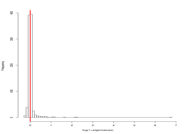
Figure 1: Distribution of the eigenvalues of the $900\times 900$ matrix obtained by the kernel of the form $\exp(-W_{2}^{2}(\mu,\nu))$. Many eigenvalues are negative, which shows that this kernel is not positive definite.

6 Conclusion and Future Directions

In this work, we have provided a theoretical way to use Wasserstein barycenters in order to define general kernels using optimal transportation maps. Considering the distance between the optimal transportation maps provide a natural way to quantify correlations between the values of a process indexed by the distribution and provides a generalization to multi-dimensional case of the work in Bachoc et al. (2018a). Using barycenter requires that the distributions are drawn according to the same measure over the set of distributions. This restricts the framework of the study to the case where the Gaussian process is defined on the support of this measure. For applications, this does not a play a too important feature since inputs are often simulated according to a specified distribution. Yet for theoretical issues, this sets the frame of this study to the infill case and not the asymptotic frame. In this case, few results exist in the statistical literature on Kriging, and thus we focused on micro-ergodicity of the parameters, proving that consistent estimate can be studied.
Finally contrary to the one-dimensional case, computational issues arise naturally when the Wasserstein distance is required. Hence the computation of a barycenter with respect to Wasserstein distance is a difficult optimization program, unless the distributions are Gaussian, leading to tractable computations as shown in Section 4. Yet this idea of linearization around the barycenter to obtain a valid covariance kernel could be used and generalized to regularized Wasserstein distance using methods proposed in Cuturi and Doucet (2014) for instance to provide a more tractable way of building kernels.

Acknowledgments: the authors would like to thank Drs. Jean Baccou and Frédéric Pérales (respectively at LIMAR and LPTM, Institut de Radioprotection et de Sûreté Nucléaire, Saint-Paul-lès-Durance, France) for the CASTEM data set, and Dr. Clément Chevalier (now with the Swiss Statistical Office, Neuchâtel, Switzerland) who has been involved in investigations on this data set in the framework of the ReDICE consortium.

Appendix A Proofs

Proof of Propositions 1 and 2

Proof.

For both propositions, only the fact that 1. implies 2. needs to be proved. Let us now do this.

Let $f_{1},\dots,f_{n}$ in $H$ and consider the matrix $\widetilde{C}=((f_{i},f_{j})_{H})_{\{i,j\}}$. This matrix is a Gram matrix in $\mathbb{R}^{n\times n}$ hence there exists a non negative diagonal matrix $D$ and an orthogonal matrix $P$ such that

$$\widetilde{C}=PDP^{{}^{\prime}}=PD^{1/2}D^{1/2}P^{{}^{\prime}}.$$

Let $e_{1},\dots,e_{n}$ be the canonical basis of $\mathbb{R}^{n}$. Then

$$e_{i}\widetilde{C}e_{j}^{{}^{\prime}}=u_{i}u_{j}^{{}^{\prime}}$$

where $u_{i}=e_{i}PD^{1/2}.$ Note that the $u_{i}$’s are vectors in $\mathbb{R}^{n}$ that depend on the $f_{1},\dots,f_{n}$. By polarization, we hence get that $(f_{i},f_{j})_{H}=(u_{i},u_{j})$ where $(,)$ denotes the usual scalar product on $\mathbb{R}^{n}$. Hence we get that for any elements $f_{1},\dots,f_{n}$ in $H$ there are $u_{1},\dots,u_{n}$ in $\mathbb{R}^{n}$ such that $\|f_{i}-f_{j}\|_{H}=\|u_{i}-u_{j}\|.$ So any covariance matrix that can be written as $[F(\|f_{i}-f_{j}\|_{H})]_{i,j}$ can be seen as a covariance matrix $[F(\|u_{i}-u_{j}\|)]_{i,j}$ on $\mathbb{R}^{n}$ and inherits its properties. The invertibility and non-negativity of this covariance matrix entail the invertibility and non-negativity of the first one, which proves the results. ∎

Proof of Theorem 3

Proof.

Without loss of generality, we can assume that $h_{0}=0\in H$. Let $\theta_{1},\theta_{2}\in\varTheta$, with $\theta_{1}\neq\theta_{2}$. Then, there exists $t^{*}\in[0,L]$ so that $F_{\theta_{1}}(0)-F_{\theta_{1}}(2t^{*})\neq F_{\theta_{2}}(0)-F_{\theta_{2}}(2t^{*})$.

For any $n\in\mathbb{N}$, let $e_{1},...,e_{n}\in H$ satisfy $(e_{i},e_{j})_{H}=\mathbf{1}_{i=j}$. Consider the $2n$ elements $(f_{1},...,f_{2n})$ made by the pairs $(-t^{*}e_{i},t^{*}e_{i})$ for $i=1,\dots,n$. Consider a Gaussian process $Y$ on $\overline{\mathcal{B}}_{2,L}$ with mean function zero and covariance function $K_{\theta_{1}}$. Then, the Gaussian vector $Z=(Y(f_{i}))_{i=1,...,2n}$ has covariance matrix $C$ given by

$$C_{i,j}=\begin{cases}F_{\theta_{1}}(0)&\mbox{if }i=j\\ F_{\theta_{1}}(2t^{*})&\mbox{if $i$ even and $j=i+1$}\\ F_{\theta_{1}}(2t^{*})&\mbox{if $i$ odd and $j=i-1$}\\ F_{\theta_{1}}(\sqrt{2}t^{*})&\mbox{else}.\end{cases}$$

Hence, we have $C=D+M$ where $M$ is the matrix with all components equal to $K_{\theta_{1}}(\sqrt{2}t^{*})$ and where $D$ is block diagonal, composed of $n$ blocks of size $2\times 2$, with each block equal to

$$B_{2,2}=\begin{pmatrix}F_{\theta_{1}}(0)-F_{\theta_{1}}(\sqrt{2}t^{*})&F_{\theta_{1}}(2t^{*})-F_{\theta_{1}}(\sqrt{2}t^{*})\\ F_{\theta_{1}}(2t^{*})-F_{\theta_{1}}(\sqrt{2}t^{*})&F_{\theta_{1}}(0)-F_{\theta_{1}}(\sqrt{2}t^{*})\end{pmatrix}.$$

Hence, in distribution, $Z=M+E$, with $M$ and $E$ independent, $M=(z,....,z)$ where $z\sim\mathcal{N}(0,K_{\theta_{1}}(\sqrt{2}t^{*}))$ and where the $n$ pairs $(E_{2k+1},E_{2k+2})$, $k=0,...,n-1$ are independent, with distribution $\mathcal{N}(0,B_{2,2})$. Hence, with $\overline{Z}_{1}=(1/n)\sum_{k=0}^{n-1}Z_{2k+1}$, $\overline{Z}_{2}=(1/n)\sum_{k=0}^{n-1}Z_{2k+2}$ and $\overline{E}=(1/n)\sum_{k=0}^{n-1}(E_{2k+1},E_{2k+2})^{t}$, we have

$$\widehat{B} :=\frac{1}{n}\sum_{i=0}^{n-1}\begin{pmatrix}Z_{2i+1}-\overline{Z}_{1}\\ Z_{2i+2}-\overline{Z}_{2}\end{pmatrix}\begin{pmatrix}Z_{2i+1}-\overline{Z}_{1}\\ Z_{2i+2}-\overline{Z}_{2}\end{pmatrix}^{t}$$

$$=\frac{1}{n}\sum_{i=0}^{n-1}\begin{pmatrix}E_{2i+1}\\ E_{2i+2}\end{pmatrix}\begin{pmatrix}E_{2i+1}\\ E_{2i+2}\end{pmatrix}^{t}-\overline{E}\overline{E}^{t}$$

$$\to_{n\to\infty}^{p}B_{2,2}.$$

Hence, there exists a subsequence $n^{\prime}\to\infty$ so that, almost surely $\widehat{B}\to B_{2,2}$ as $n^{\prime}\to\infty$. Hence, almost surely $\widehat{B}_{11}-\widehat{B}_{1,2}\to K_{\theta_{1}}(0)-K_{\theta_{1}}(2t^{*})$ as $n^{\prime}\to\infty$. Hence, the set

$$A=\left\{g\in\overline{F};\widehat{B}_{2,2}\left(g(f_{1}),....g(f_{2n^{\prime}})\right)\to_{n^{\prime}\to\infty}F_{\theta_{1}}(0)-F_{\theta_{1}}(2t^{*})\right\}$$

satisfies $P_{\theta_{1}}(A)=1$. With the same arguments, we can show $P_{\theta_{2}}(B)=1$, where

$$B=\left\{g\in\overline{F};\widehat{B}_{2,2}\left(g(f_{1}),....g(f_{2n^{\prime\prime}})\right)\to_{n^{\prime\prime}\to\infty}F_{\theta_{2}}(0)-F_{\theta_{2}}(2t^{*})\right\}$$

where $n^{\prime\prime}$ is a subsequence extracted from $n^{\prime}$. Since $A\cap B=\varnothing$, it follows that $P_{\theta_{2}}(A)=0$. Hence, $\theta$ is microergodic.

∎

Proof of Proposition 4

Recall that the empirical barycenters $\,(\overline{\mu}_{n})_{n}\,$ is a sequence of continuous measures converging to $\,\overline{\mu}\,$ in $\,2\,$-Wasserstein distance: $\,W_{2}(\overline{\mu}_{n},\overline{\mu})\rightarrow 0\,$ as $\,n\rightarrow\infty\,$ and $\,R_{n\sharp}\overline{\mu}=\overline{\mu}_{n}\,$ with $W_{2}^{2}(\overline{\mu},\overline{\mu}_{n})=||R_{n}||_{L^{2}(\overline{\mu})}$.

Lemma 1.

Fix some distribution $\,\nu\,$ absolutely continuous with respect to Lebesgue measure and let $T=T_{\nu}$ and $T_{n}=T_{\nu,n}$. Then it holds a.s.

$$\bigl{\|}T-T_{n}\bigr{\|}^{2}_{L^{2}(\nu)}\longrightarrow 0,~{}\text{as}~{}n\rightarrow\infty.$$

Proof.

Fix $\,n\,$ s.t. $\,W_{2}(\overline{\mu}_{n},\overline{\mu})=\varepsilon_{n}\,$. Consider $\,\bigl{\|}\text{id}-R_{n}\circ T\bigr{\|}_{L^{2}(\nu)}\,$. By change of variables and triangle inequality one obtains

$$\bigl{\|}\text{id}-R_{n}\circ T\bigr{\|}_{L^{2}(\nu)} =\bigl{\|}T^{-1}-R_{n}\bigr{\|}_{L^{2}(\overline{\mu})}\leq\bigl{\|}T^{-1}-\text{id}\bigr{\|}_{L^{2}(\overline{\mu})}+\bigl{\|}R_{n}-\text{id}\bigr{\|}_{L^{2}(\overline{\mu})}$$

$$\leq W_{2}(\nu,\overline{\mu})+\varepsilon_{n}\leq W_{2}(\nu,\overline{\mu}_{n})+2\varepsilon_{n}.$$

Since $T_{n}$ is the optimal transport map from $\nu$ to $\mu_{n}$ we recall that $W_{2}(\nu,\overline{\mu}_{n})=\bigl{\|}\text{id}-T_{n}\bigr{\|}_{L^{2}(\nu)}$. So due to the arbitrary choice of $\,n\,$ it follows

$$\Bigl{|}\bigl{\|}\text{id}-R_{n}\circ T\bigr{\|}_{L^{2}(\nu)}-\bigl{\|}\text{id}-T_{n}\bigr{\|}_{L^{2}(\nu)}\Bigr{|}\underset{n\rightarrow\infty}{\longrightarrow}0.$$ (A.1)

Now we are ready to prove, that $\,\bigl{\|}T_{n}-T\bigr{\|}_{L^{2}(\nu)}\overset{n\rightarrow\infty}{\longrightarrow}0\,$. Assume the claim is wrong. Assume the claim is wrong:

$$T_{n}\overset{n\rightarrow\infty}{\longrightarrow}T_{1},\quad R_{n}\circ T\overset{n\rightarrow\infty}{\longrightarrow}T_{2},\quad\|T_{1}-T_{2}\|>\varepsilon.$$

Thus

$$\bigl{\|}\text{id}-T_{n}\bigr{\|}_{L^{2}(\nu)}\overset{n\rightarrow\infty}{\longrightarrow}\bigl{\|}\text{id}-T_{1}\bigr{\|}_{L^{2}(\nu)},\quad\bigl{\|}\text{id}-R_{n}\circ T\bigr{\|}_{L^{2}(\nu)}\overset{n\rightarrow\infty}{\longrightarrow}\bigl{\|}\text{id}-T_{2}\bigr{\|}_{L^{2}(\nu)},$$

which contradicts to (A.1) ∎

The next lemma is a key ingredient in the proof of the fact that the true kernel can be replaced by its empirical counterpart.

Lemma 2.

Consider two fixed absolutely continuous measures $\mu$ and $\nu$ in $\mathcal{W}_{2}(\mathbb{R}^{p})$. We have a.s.

$$\Bigl{|}\bigl{\|}T_{\mu}^{-1}-T_{\nu}^{-1}\bigr{\|}^{2}_{L^{2}(\overline{\mu})}-\bigl{\|}T^{-1}_{\mu,n}-T^{-1}_{\nu,n}\bigr{\|}^{2}_{L^{2}(\overline{\mu}_{n})}\Bigr{|}\longrightarrow 0,~{}\text{as}~{}n\rightarrow\infty.$$

Proof.

Consider $\,\bigl{\|}T^{-1}_{\mu,n}-T^{-1}_{\nu,n}\bigr{\|}_{L^{2}(\overline{\mu}_{n})}\,$. Change of variables and triangle inequality yield

$$\bigl{\|}T^{-1}_{\mu,n}-T^{-1}_{\nu,n}\bigr{\|}_{L^{2}(\overline{\mu}_{n})}=\bigl{\|}T^{-1}_{\mu,n}\circ R_{n}-T^{-1}_{\nu,n}\circ R_{n}\bigr{\|}_{L^{2}(\overline{\mu})}$$

$$\leq\bigl{\|}T^{-1}_{\mu,n}\circ R_{n}-T^{-1}_{\mu}\bigr{\|}_{L^{2}(\overline{\mu})}+\bigl{\|}T^{-1}_{\nu,n}\circ R_{n}-T_{\nu}^{-1}\bigr{\|}_{L^{2}(\overline{\mu})}+\bigl{\|}T^{-1}_{\mu}-T_{\nu}^{-1}\bigr{\|}_{L^{2}(\overline{\mu})}.$$

Therefore one obtains

$$\bigl{\|}T^{-1}_{\mu,n}-T^{-1}_{\nu,n}\bigr{\|}_{L^{2}(\overline{\mu}_{n})}-\bigl{\|}T^{-1}_{\mu}-T_{\nu}^{-1}\bigr{\|}_{L^{2}(\overline{\mu})}$$

$$\leq\bigl{\|}T^{-1}_{\nu,n}\circ R_{n}-T_{\nu}^{-1}\bigr{\|}_{L^{2}(\overline{\mu})}+\bigl{\|}T^{-1}_{\mu,n}\circ R_{n}-T_{\mu}^{-1}\bigr{\|}_{L^{2}(\overline{\mu})}\overset{n\rightarrow\infty}{\longrightarrow}0$$

where the last relation holds due to Lemma 1. ∎

Proof of Proposition 5

Proof.

Actually using Lemma A.2 together with Theorem 2.2 in Kroshnin et al. (2019), we obtain that

$$\|R_{n}-{\rm Id}\|_{L^{2}(\overline{\mu})}=O_{P}\left(\frac{1}{\sqrt{n}}\right),$$

and that the empirical transportation plan can be linearized as

$$T_{i,n}^{-1}=T_{i}^{-1}+D(\overline{S}_{n}-\overline{S})+o(\|\overline{S}_{n}-\overline{S}\|_{F}),$$

where $D$ is a linear self-adjoint bounded operator acting on the space of symmetric matrices. Use the following decomposition

$$\|T_{i,n}^{-1}\circ R_{n}-T_{i}^{-1}\|_{L^{2}(\overline{\mu})}\leq \|T_{i}^{-1}\circ R_{n}-T_{i}^{-1}+(T_{i,n}^{-1}-T_{i}^{-1})\circ R_{n}\|_{L^{2}(\overline{\mu})}$$

$$\leq \|T_{i}^{-1}\circ R_{n}-T_{i}^{-1}\|_{L^{2}(\overline{\mu})}+\|(T_{i,n}^{-1}-T_{i}^{-1})\circ R_{n}\|_{L^{2}(\overline{\mu})}$$

$$\leq O_{P}\left(\frac{1}{\sqrt{n}}\right).$$

This entails that $\|T_{i,n}^{-1}\ -T_{j,n}^{-1}\|_{L^{2}(\overline{\mu}_{n})}-\|T_{i}^{-1}\ -T_{j}^{-1}\|_{L^{2}(\overline{\mu})}$ is also of order $\frac{1}{\sqrt{n}}$ since

$$\bigl{\|}T^{-1}_{i,n}-T^{-1}_{j,n}\bigr{\|}_{L^{2}(\overline{\mu}_{n})}-\bigl{\|}T^{-1}_{i}-T_{j}^{-1}\bigr{\|}_{L^{2}(\overline{\mu})}\leq\bigl{\|}T^{-1}_{i,n}\circ R_{n}-T^{-1}_{i}\bigr{\|}_{L^{2}(\overline{\mu})}+\bigl{\|}T^{-1}_{j,n}\circ R_{n}-T_{j}^{-1}\bigr{\|}_{L^{2}(\overline{\mu})}$$

Since for all $(i,j)\in[1,N]$,

$$K_{n}(i,j)=F(\|T_{i,n}^{-1}-T_{j,n}^{-1}\|^{2}_{L^{2}(\overline{\mu}_{n})})$$

as soon as $F$ is continuously differentiable with bounded derivative, then we get that for a finite constant

$$\sum_{i,j=1}^{N}|K_{n}(i,j)-K(i,j)|^{2}\leq N^{2}\sup_{i,j}|K_{n}(i,j)-K(i,j)|^{2}\leq C\frac{N^{2}}{n},$$

which concludes the proof. ∎

Proof of Proposition 6

Proof.

Note, that for any orthogonal matrix $\,U\,$ the following set of inequalities hold:

$$W^{2}_{2}\left(\mathcal{N}(0,S),\mathcal{N}(0,Q)\right) :=\text{tr}(S)+\text{tr}(Q)-2\text{tr}\left(Q^{1/2}SQ^{1/2}\right)^{1/2}$$

$$=W^{2}_{2}\left(\mathcal{N}(0,USU^{T}),\mathcal{N}(0,UQU^{T})\right)$$

$$=W^{2}_{2}\left(\phi_{U}(\mathcal{N}(0,S)),\phi_{U}(\mathcal{N}(0,Q))\right).$$

Thus, map $\,\phi_{U}\,$ preserves $\,2\,$-Wasserstein distance. Equality (4.4) follows from  (4.3) by substituting $\,S_{i}\,$, $\,S_{j}\,$, and $\,\overline{S}\,$ by $\,US_{i}U^{T}\,$, $\,US_{j}U^{T}\,$, and $\,U\overline{S}U^{T}\,$ respectively. ∎

References

- Abrahamsen (1997) P. Abrahamsen. A review of Gaussian random fields and correlation functions. Technical report, Norwegian computing center, 1997.
- Agueh and Carlier (2011) Martial Agueh and Guillaume Carlier. Barycenters in the wasserstein space. SIAM Journal on Mathematical Analysis, 43(2):904–924, 2011.
- Alvarez-Esteban et al. (2015) Pedro C Alvarez-Esteban, E del Barrio, JA Cuesta-Albertos, and C Matrán. Wide consensus for parallelized inference. arXiv preprint arXiv:1511.05350, 2015.
- Álvarez-Esteban et al. (2016) Pedro C. Álvarez-Esteban, E. del Barrio, J.A. Cuesta-Albertos, and C. Matrán. A fixed-point approach to barycenters in wasserstein space. Journal of Mathematical Analysis and Applications, 441(2):744 – 762, 2016. ISSN 0022-247X. https://doi.org/10.1016/j.jmaa.2016.04.045. URL http://www.sciencedirect.com/science/article/pii/S0022247X16300907.
- Anderes (2010) E. Anderes. On the consistent separation of scale and variance for Gaussian random fields. The Annals of Statistics, 38:870–893, 2010.
- Bachoc (2013) François Bachoc. Cross validation and maximum likelihood estimations of hyper-parameters of gaussian processes with model misspecification. Computational Statistics & Data Analysis, 66:55–69, 2013.
- Bachoc et al. (2018a) François Bachoc, Fabrice Gamboa, Jean-Michel Loubes, and Nil Venet. A gaussian process regression model for distribution inputs. IEEE Transactions on Information Theory, 64(10):6620–6637, 2018a.
- Bachoc et al. (2018b) François Bachoc et al. Asymptotic analysis of covariance parameter estimation for gaussian processes in the misspecified case. Bernoulli, 24(2):1531–1575, 2018b.
- Bevilacqua et al. (2016) Moreno Bevilacqua, Tarik Faouzi, Reinhard Furrer, and Emilio Porcu. Estimation and prediction using generalized wendland covariance functions under fixed domain asymptotics. arXiv preprint arXiv:1607.06921, 2016.
- Bigot and Klein (2012) J. Bigot and T. Klein. Characterization of barycenters in the Wasserstein space by averaging optimal transport maps. ArXiv e-prints, December 2012.
- Boeckel et al. (2018) Melf Boeckel, Vladimir Spokoiny, and Alexandra Suvorikova. Multivariate brenier cumulative distribution functions and their application to non-parametric testing. arXiv preprint arXiv:1809.04090, 2018.
- Boissard et al. (2015) Emmanuel Boissard, Thibaut Le Gouic, Jean-Michel Loubes, et al. Distribution’ s template estimate with wasserstein metrics. Bernoulli, 21(2):740–759, 2015.
- Borchers (2016) H Borchers. adagio: Discrete and global optimization routines. URL http://CRAN. R-project. org/package= adagio, 2016.
- Brenier (1991) Y. Brenier. Polar factorization and monotone rearrangement of vector-valued functions. Communications on pure and applied mathematics, 44(4):375–417, 1991.
- Chernozhukov et al. (2017) Victor Chernozhukov, Alfred Galichon, Marc Hallin, Marc Henry, et al. Monge–kantorovich depth, quantiles, ranks and signs. The Annals of Statistics, 45(1):223–256, 2017.
- Cristianini and Shawe-Taylor (2000) Nello Cristianini and John Shawe-Taylor. Support Vector Machines. Cambridge University Press, 2000.
- Cuesta and Matrán (1989) Juan Antonio Cuesta and Carlos Matrán. Notes on the Wasserstein metric in Hilbert spaces. Ann. Probab., 17(3):1264–1276, 1989. ISSN 0091-1798. URL http://links.jstor.org/sici?sici=0091-1798(198907)17:3<1264:NOTWMI>2.0.CO;2-J&origin=MSN.
- Cuturi and Doucet (2014) Marco Cuturi and Arnaud Doucet. Fast computation of wasserstein barycenters. In International Conference on Machine Learning, pages 685–693, 2014.
- del Barrio et al. (2018) Eustasio del Barrio, Juan A. Cuesta-Albertos, Marc Hallin, and Carlos Matrán. Center-Outward Distribution Functions, Quantiles, Ranks, and Signs in . arXiv e-prints, art. arXiv:1806.01238, Jun 2018.
- Figalli (2018) Alessio Figalli. On the Continuity of Center-Outward Distribution and Quantile Functions. arXiv e-prints, art. arXiv:1805.04946, May 2018.
- Ginsbourger et al. (2016) David Ginsbourger, Jean Baccou, Clément Chevalier, and Frédéric Perales. Design of computer experiments using competing distances between set-valued inputs. In mODa 11-Advances in Model-Oriented Design and Analysis, pages 123–131. Springer, 2016.
- Gottschlich and Schuhmacher (2014) Carsten Gottschlich and Dominic Schuhmacher. The shortlist method for fast computation of the earth mover’s distance and finding optimal solutions to transportation problems. PloS one, 9(10):e110214, 2014.
- (23) http://www cast3m.cea.fr. Cast3m software.
- Klatt (2018) Marcel Klatt. Regularized Wasserstein Distances and Barycenters, 2018. URL https://cran.r-project.org/web/packages/Barycenter/Barycenter.pdf. R package version 1.3.1.
- Kolouri et al. (2015) Soheil Kolouri, Yang Zou, and Gustavo K. Rohde. Sliced Wasserstein kernels for probability distributions. CoRR, abs/1511.03198, 2015. URL http://arxiv.org/abs/1511.03198.
- Kroshnin et al. (2019) Alexey Kroshnin, Vladimir Spokoiny, and Alexandra Suvorikova. Statistical inference for bures-wasserstein barycenters. arXiv preprint arXiv:1901.00226, 2019.
- Le Gouic and Loubes (2017) Thibaut Le Gouic and Jean-Michel Loubes. Existence and consistency of wasserstein barycenters. Probability Theory and Related Fields, 168(3-4):901–917, 2017.
- Loh (2015) Wei-Liem Loh. Estimating the smoothness of a gaussian random field from irregularly spaced data via higher-order quadratic variations. The Annals of Statistics, 43(6):2766–2794, 2015.
- Luenberger et al. (1984) David G Luenberger, Yinyu Ye, et al. Linear and nonlinear programming, volume 2. Springer, 1984.
- Mérigot (2011) Quentin Mérigot. A multiscale approach to optimal transport. In Computer Graphics Forum, volume 30, pages 1583–1592. Wiley Online Library, 2011.
- Micchelli et al. (2006) Charles A Micchelli, Yuesheng Xu, and Haizhang Zhang. Universal kernels. Journal of Machine Learning Research, 7(Dec):2651–2667, 2006.
- Muandet et al. (2016) K. Muandet, K. Fukumizu, B. Sriperumbudur, and B. Schölkopf. Kernel Mean Embedding of Distributions: A Review and Beyonds. ArXiv e-prints, May 2016.
- Peyré et al. (2019) Gabriel Peyré, Marco Cuturi, et al. Computational optimal transport. Foundations and Trends® in Machine Learning, 11(5-6):355–607, 2019.
- Poczos et al. (2013) Barnabas Poczos, Aarti Singh, Alessandro Rinaldo, and Larry Wasserman. Distribution-free distribution regression. In Carlos M. Carvalho and Pradeep Ravikumar, editors, Proceedings of the Sixteenth International Conference on Artificial Intelligence and Statistics, volume 31 of Proceedings of Machine Learning Research, pages 507–515, Scottsdale, Arizona, USA, 29 Apr–01 May 2013. PMLR. URL http://proceedings.mlr.press/v31/poczos13a.html.
- Rasmussen (2004) Carl Edward Rasmussen. Gaussian processes in machine learning. In Advanced lectures on machine learning, pages 63–71. Springer, 2004.
- Rasmussen and Williams (2006) C.E. Rasmussen and C.K.I. Williams. Gaussian Processes for Machine Learning. The MIT Press, Cambridge, 2006.
- Santambrogio (2015) Filippo Santambrogio. Optimal transport for applied mathematicians. Birkäuser, NY, pages 99–102, 2015.
- Santner et al. (2003) T.J Santner, B.J Williams, and W.I Notz. The Design and Analysis of Computer Experiments. Springer, New York, 2003.
- Schoenberg (1938) Isaac J Schoenberg. Metric spaces and completely monotone functions. Annals of Mathematics, pages 811–841, 1938.
- Schölkopf and Smola (2002) Bernhard Schölkopf and Alexander J Smola. Learning with kernels: support vector machines, regularization, optimization, and beyond. MIT press, 2002.
- Schuhmacher et al. (2019) Dominic Schuhmacher, Björn Bähre, Carsten Gottschlich, Valentin Hartmann, Florian Heinemann, and Bernhard Schmitzer. transport: Computation of Optimal Transport Plans and Wasserstein Distances, 2019. URL https://cran.r-project.org/package=transport. R package version 0.11-0.
- Stein (1999) M.L. Stein. Interpolation of Spatial Data: Some Theory for Kriging. Springer, New York, 1999.
- Trang Bui et al. (2018) Thi Thien Trang Bui, J-M Loubes, L Risser, and P Balaresque. Distribution regression model with a Reproducing Kernel Hilbert Space approach. arXiv e-prints, art. arXiv:1806.10493, Jun 2018.
- Uribe et al. (2018) César A. Uribe, Darina Dvinskikh, Pavel Dvurechensky, Alexander Gasnikov, and Angelia Nedić. Distributed computation of Wasserstein barycenters over networks. In 2018 IEEE 57th Annual Conference on Decision and Control (CDC), 2018. Accepted, arXiv:1803.02933.
- Villani (2009) Cédric Villani. Optimal transport: old and new, volume 338. Springer Science & Business Media, 2009.
- Wendland (2004) Holger Wendland. Scattered data approximation, volume 17. Cambridge university press, 2004.
- Zhang (2004) H. Zhang. Inconsistent estimation and asymptotically equivalent interpolations in model-based geostatistics. Journal of the American Statistical Association, 99:250–261, 2004.