Milling and meandering: Flocking dynamics of stochastically interacting agents with a field of view

Abstract

We introduce a stochastic agent-based model for the flocking dynamics of self-propelled particles that exhibit velocity-alignment interactions with neighbours within their field of view. The stochasticity in the dynamics of the model arises purely from the uncertainties at the level of interactions. Despite the absence of attractive forces, this model gives rise to a wide array of emergent patterns that exhibit long-time spatial cohesion. In order to gain further insights into the dynamical nature of the resulting patterns, we investigate the system behaviour using an algorithm that identifies spatially distinct clusters of the flock and computes their corresponding angular momenta. Our results suggest that the choice of field of view is crucial in determining the resulting emergent dynamics of stochastically interacting particles.

The collective movement of large groups of microorganisms, insects, birds, and mammals are amongst the most spectacular examples of self-organized phenomena in the natural world Vicsek2012 ; Sumpter2006 . Species across a range of length scales exhibit a rich variety of collective patterns of motion that are united by similar underlying characteristics Parrish1997 ; Menon2010 . Advances in experimental techniques for investigating flocking Cavagna2018 has sustained interest in uncovering the principles that underpin this emergent phenomenon. For instance, recent experiments have demonstrated that pairwise interactions motivated by biological goals play a crucial role in determining insect swarming patterns Puckett2015 . Flocks may fundamentally be viewed as dry active matter, namely systems of self-propelled particles that do not exhibit conservation of momentum Marchetti2013 , and their dynamics can be understood as a process similar to the long-range ordering of interacting particles Cavagna2014 . Following the seminal work of Vicsek et al. Vicsek1995 ; Ginelli2016 , the dominant paradigm in models of flocking is that stochasticity in the dynamics can be accounted for through external noise (either additive or multiplicative). However, this approach is only truly appropriate for situations such as a system of Brownian particles, where fluctuations arise from the surrounding media. In contrast, experimental evidence suggests that the dominant contribution to the stochasticity in flocks arises from variability in the behaviour of individual particles Aplin2014 ; Delgado2018 . Furthermore, the collective dynamics of a swarm is known to be density-dependent Buhl2006 ; Yates2009 , which tacitly suggests that variations in individual behaviour may have a cumulative impact. Indeed, flocks may exhibit ordered macroscopic dynamics even if the behaviour of individual particles is subject to noise Niizato2018 . Hence, it is of significant interest to consider the emergent flocking behaviour in a system where stochasticity arises purely from the uncertainties at the level of inter-particle interactions.

In situations where individual particles are unable to uniformly survey their neighbourhood due to physiological or other constraints, their interactions would be limited to neighbours that lie within a field of view Hemelrijk2012 . It has been observed that even a minimal assumption of fore-aft asymmetry can significantly impact the collective dynamics of a flock Chen2017 . Furthermore, a range of flocking patterns can be observed in a system with position-dependent short range interactions restricted by a vision cone  Barberis2016 . Recently, we demonstrated that similar constraints on the field of view of a particle in a two-dimensional lattice model of flocking can yield a jamming transition even at extremely low particle densities Menon2017 . However, the role of a field of view on the dynamics of particles that undergo stochastic velocity alignments remains an open question. Moreover, while certain types of position-dependent interactions can facilitate cohesion in a flock Gregoire2003 ; Gregoire2004 , it is intriguing to consider how this outcome might be achieved with velocity alignments alone. Furthermore, while some flocking models have incorporated the acceleration of particles to describe short-term memory Szabo2009 , collision avoidance Peng2009 , consensus decision making Bhattacharya2010 and other experimentally observed features Mishra2012 , the role of position-independent stochastic acceleration remains to be established.

In order to address these questions, we propose in this article a novel paradigm for flocking in which long-time spatial cohesion can emerge through a stochastic acceleration, despite the absence of attractive forces or explicit confinement. While there have been previous attempts at incorporating stochasticity arising from an individual particle’s evaluation of their interactions with agents in their neighbourhood (for example Chate2008 ), here we explicitly consider a situation where, at each instant, particles interact with a single randomly chosen neighbour in their field of view. We assume that the interaction between a chosen pair of particles depends only on their respective velocities, in contrast to the typical assumption of two-body or mean-field interactions that depend on the relative positions of particles. Furthermore, while most previous flocking models account for stochasticity through an external noise, here it is a consequence of uncertainty in velocity alignments. This leads to a variety of emergent collective dynamical patterns whose spatio-temporal characteristics vary significantly. Finally, in order to classify these patterns in a unified manner, we present a cluster-finding algorithm that determines the spatially distinct clusters of the flock and their associated angular momenta.

We consider an agent-based model of $N$ interacting point-like particles moving in two dimensions. The state of each agent $i$ at a time step $t$ is described by its position $\mathbf{x}_{i}(t)$ and velocity $\mathbf{v}_{i}(t)$. We define the velocity of an agent to be its displacement in a unit time step, and which therefore has the dimension of length. The dynamics of the system is governed by the following update rule: at each time step $t$, an agent $i$ interacts with a randomly chosen agent $j$ with a specified probability $p(\mathbf{x}_{j}(t),\mathbf{v}_{j}(t)|\mathbf{x}_{i}(t),\mathbf{v}_{i}(t))$, defined later, leading to a change in its velocity. If it does not find any agent to interact with, it instead moves a distance $|\mathbf{v}_{i}(t)|$ in a random direction. The velocity $\mathbf{v}_{i}(t)$ and position $\mathbf{x}_{i}(t)$ are updated as

$$\mathbf{v}_{i}(t+1) =\mathbf{v}_{i}(t)+\mathbf{a}_{i}(t)\,,$$ (1a)

$$\mathbf{x}_{i}(t+1) =\mathbf{x}_{i}(t)+\mathbf{v}_{i}(t+1)\,.$$ (1b)

Here $\mathbf{a}_{i}(t)$ is the acceleration of the agent, and is given by

$$\mathbf{a}_{i}(t) =\left\{\begin{array}[]{ll}-\mathbf{v}_{i}(t)+|\mathbf{v}_{i}(t)|\,\hat{\bm{\eta}},&\text{if~{}}\Omega_{i}=\emptyset,\\ \alpha[\mathbf{v}_{j}(t)-\mathbf{v}_{i}(t)+f(\mathbf{v}_{j}(t)+\mathbf{v}_{i}(t))],&\text{otherwise},\end{array}\right.$$ (4)

where $\Omega_{i}$ is the set of all agents with which agent $i$ may interact with, the coefficient $\alpha<1$ is the strength of interaction, and $\hat{\bm{\eta}}$ is a chosen from a uniform random distribution of vectors on the unit circle. The initial condition is specified as $\mathbf{x}_{i}(0)=\mathbf{x}_{i}^{0}$ and $\mathbf{v}_{i}(0)=\mathbf{v}_{i}^{0}$ for all $i=1,2,\ldots N$.

We note from Eq. (1a) that when $\Omega_{i}\neq\emptyset$, the velocity update is dependent on the randomly chosen agent $j$. The linear term $\alpha(\mathbf{v}_{j}-\mathbf{v}_{i})$ in Eq. (4) describes an alignment interaction, while the nonlinear term $f(\mathbf{v}_{j}+\mathbf{v}_{i})$ keeps the velocity close to a critical value $\mathbf{v}_{c}$, i.e. it ensures that the flock maintains a constant average speed. Assuming $|\mathbf{v}_{c}|=1$, we consider $f(\mathbf{v}):=\mathbf{v}(1-|\mathbf{v}|)/(1+|\mathbf{v}|^{\beta})$ with $\beta=3$ (see Supplementary Information for a more detailed discussion).

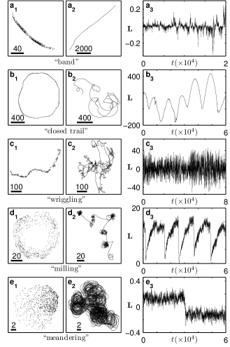
Figure 1: Examples of the spatially contiguous dynamical flocking patterns exhibited by the model for a system of $N=10^{3}$ agents. In each row the left panel displays a snapshot of the flock, the right panel displays the angular momentum per particle $\mathbf{L}$ over a duration of time, and the middle panel displays the corresponding trajectory of the center of mass of the flock $\bar{\mathbf{x}}(t)$ over the same duration. (a₁-a₃) Agents moving in a band for the case $\sigma=6$, $\theta_{\max}=90$ and $\alpha=0.1$. (b₁-b₃) Agents moving in a wriggling pattern for the case $\sigma=5$, $\theta_{\max}=40$ and $\alpha=0.8$. (c₁-c₃) Agents moving in a closed trail for the case $\sigma=3$, $\theta_{\max}=50$ and $\alpha=0.1$. (d₁-d₃) Agents moving in a milling pattern for the case $\sigma=1$, $\theta_{\max}=20$ and $\alpha=0.025$. (e₁-e₃) Agents moving in a flock with a meandering center of mass for the case $\sigma=3$, $\theta_{\max}=15$ and $\alpha=0.02$. The numbered solid bars in the left and middle panels of every row provides a measure of spatial distance in each case.

For our current investigation, we assume that every agent $i$ has a field of view, symmetric around its direction of motion, that is delimited by a maximum bearing angle $\theta_{\max}$. The probability $p(\mathbf{x}_{j},\mathbf{v}_{j}|\mathbf{x}_{i},\mathbf{v}_{i})$ that an agent $i$ interacts with an agent $j\in\Omega_{i}$ may be specified in terms of weights $\omega_{i,j}$. We assume that a given agent mostly interacts with agents separated from it by an optimal interaction length, and that the probability that it randomly selects an agent lying very close to, or very far away from itself is negligible. With these properties in mind we assume the following weight function

$$\omega_{i,j}=|\mathbf{x}_{i}-\mathbf{x}_{j}|\,e^{-\frac{|\mathbf{x}_{i}-\mathbf{x}_{j}|^{2}}{2\sigma^{2}}}\left(1-{\theta_{i,j}^{2}}/{\theta_{\max}^{2}}\right)\,,$$ (5)

if $\theta_{i,j}\leq\theta_{\max}$ and $\omega_{i,j}=0$ for $\theta_{i,j}>\theta_{\max}$, where $\sigma$ is the mean interaction length and $\theta_{i,j}$ is the angle between the velocity $\mathbf{v}_{i}$ and the vector $\mathbf{x}_{j}-\mathbf{x}_{i}$. Given this weight function, the probability can be written as $p(\mathbf{x}_{j},\mathbf{v}_{j}|\mathbf{x}_{i},\mathbf{v}_{i})=\omega_{i,j}/\sum_{k\in\Omega_{i}}\omega_{ik}$.

In the limiting case $\theta_{\max}=\pi$, there are no random rotations as, by definition, we would have $\Omega_{i}\neq\emptyset\;\forall\;i$. In this situation any initial randomness will eventually get redistributed over the whole population, and it is expected that the velocities will converge to that of the initial mean velocity. Furthermore, here an agent $i$ has the highest likelihood to align with any neighbour $j$ that approximately lies at a distance $|\mathbf{x}_{i}-\mathbf{x}_{j}|=\sigma$ (i.e. where $\omega_{i,j}$ is at its maximum). Hence, in our simulations we assume that the initial positions $\mathbf{x}_{i}^{0}$ are selected randomly over a small region of size $\sim\mathcal{O}(\sigma)$ and velocities $\mathbf{v}_{i}^{0}$ are chosen from a uniform distribution.

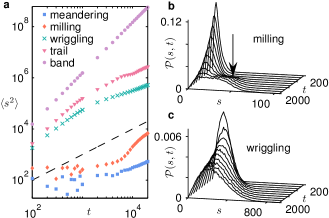
Figure 2: Statistics of the center of mass trajectories (a) Time-dependence of the average mean-squared displacement (MSD) of the center of mass $\langle s^{2}\rangle$, calculated over $10^{4}$ trials, for each of the five sets of parameter values considered in Fig. 1. The dashed line, shown for reference, indicates the MSD for the case of normal diffusion. (b-c) The probability distribution function $\mathpzc{P}(s,t)$, calculated over $5\times 10^{4}$ trials, shown over a range of displacements $s$ and time $t$ for the cases (b) $\sigma=1$, $\theta_{\max}=20$, $\alpha=0.025$ (a milling pattern), and (c) $\sigma=5$, $\theta_{\max}=40$, $\alpha=0.8$ (a wriggling pattern). The arrow in panel (b) indicates a large excursion.

Upon varying the interaction strength $\alpha$, mean interaction length $\sigma$ and the maximum bearing angle $\theta_{\rm max}$ over a range of values for a system of $N=10^{3}$ agents, we find that the model exhibits a wide range of patterns (see Fig. 1). From our numerical simulations, we find that the resulting patterns can sustain their cohesiveness over a very long period of time ($t\gtrsim 10^{6}$ steps). These observed patterns include an extended band-like flock that can move ballistically for long durations (Fig. 1(a)), a spatially extended wriggling pattern (Fig. 1(b)), a very large and narrow closed trail pattern (Fig. 1(c)), a flock that exhibits a milling, or vortex-like, pattern (Fig. 1(d)), and a flock with a meandering center of mass, and rotating profile, that remains confined to a small region of space (Fig. 1(e)). Movies of the patterns displayed in Fig. 1(b₁-e₁) are included as Supplementary Information. Furthermore, in addition to the patterns displayed in Fig. 1, this system can exhibit multiple interacting clusters. To illustrate this we have plotted in Fig. 1(a₃-e₃) the temporal variation of the angular momentum per particle, $\mathbf{L}=N^{-1}\sum_{i}(\mathbf{x}_{i}-\bar{\mathbf{x}})\times\mathbf{v}_{i}$ for the corresponding flocking patterns, where $\bar{\mathbf{x}}(t)=N^{-1}\sum_{i}\mathbf{x}_{i}(t)$ is the center of mass of the flock. We observe that this quantity exhibits remarkably distinct temporal profiles for each of the displayed patterns, and captures the spontaneous switching/reversal in the direction of rotation of the flock, which manifests as a change in the sign of $\mathbf{L}$.

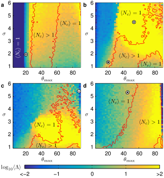
Figure 3: Parameter space diagrams obtained using the cluster-finding algorithm described in the text. The ensemble-averaged quantities $\langle N_{c}\rangle$ and $\langle\mathbf{\Lambda}\rangle$ are computed over a range of values of the mean interaction length $\sigma$, interaction strength $\alpha$ and the maximum bearing angle $\theta_{\max}$, and are averaged over $10$ trials. The four panels correspond to (a) $\alpha=0.01$, (b) $\alpha=0.05$, (c) $\alpha=0.1$ and (d) $\alpha=0.5$. In each, we display (in log-scale) the dependence of the average angular momentum of the flock $\langle\mathbf{\Lambda}\rangle$ on system parameters, along with contour lines that demarcate the regimes where the flock is characterized by a single cluster ($\langle N_{c}\rangle=1$) and multiple clusters ($\langle N_{c}\rangle>1$). The black markers within white circles in each panel indicate locations in the parameter space where we observe a meandering pattern (a: plus sign), a milling pattern (b: filled square), a closed trail (b: cross), a band pattern (c: filled circle) and a wriggling pattern (d: filled triangle). A more detailed exploration of the parameter space, with snapshots of the patterns obtained, is provided in the Supplementary Information.

In Fig. 1(a₂-e₂), the trajectories of the center of mass of the flock, $\bar{\mathbf{x}}(t)$, illustrate the diversity of collective dynamics that this model is capable of exhibiting. These range from near-ballistic motion in the case of the band-like patterns (Fig. 1(a2)) to winding behaviour with occasional long excursions, similar to that of a correlated random walk, in the case of the milling pattern (Fig. 1(e2)). To discern the macroscopic features of these trajectories, we discard an initial transient period of duration $t_{0}=10^{3}$ and compute the probability distribution function $\mathpzc{P}(s,t)$, where $s=|\bar{\mathbf{x}}(t)-\bar{\mathbf{x}}(t_{0})|$, and the mean square displacement (MSD) of the center of mass, $\langle s^{2}\rangle$. While the trail and wriggling patterns show a superdiffusive behaviour at small time scales, they appear to converge to normal diffusion $\langle s^{2}\rangle\sim t$ asymptotically (cf. dashed line in Fig. 2(a)). In contrast, the milling and the meandering patterns are initially subdiffusive and asymptotically converge to normal diffusion, while the band pattern is superdiffusive at all times. The probability density function $\mathpzc{P}(s,t)$ for the milling and the wriggling patterns are shown in Fig. 2(b) and (c). We find that the patterns show a qualitatively similar decay of $\mathpzc{P}(s,t)$ at small times. However, as indicated by an arrow in Fig. 2(b), the center of mass of the milling pattern exhibits a higher probability of large excursions at later times, which corresponds to intervals where rotation ceases due to an internal reorganization of the flock.

It is apparent from the breadth of complexity of the observed flocking patterns that simple order parameters, such as the mean velocity of the flock, would be insufficient to characterize the dynamics of the model. While a non-zero mean velocity, corresponding to ordered motion, may indicate the existence of the band pattern, a zero mean velocity may either correspond to diffusive randomly moving agents or to an ordered rotating swirl. Furthermore, we find that the flock may be characterized by several clusters for certain choices of the system parameters. Hence, we would require a set of order parameters that could more accurately distinguish between the wide array of flocking patterns observed in our simulations

To this end, we classify the patterns in terms of the number of distinct (contiguous) clusters and their associated angular momenta at a given time, through a cluster-finding algorithm. This procedure, which we rigorously detail in the Supplementary Information, is outlined as follows. We define the resolution length $R=\lambda R_{\max}$, where $0<\lambda\leq 1$, and $R_{\max}$ is the maximum separation between any two particles in the flock at time $t$. At the length scale $R_{\max}$ the system can be viewed as comprising a single cluster that encompasses the entire flock. For the chosen length scale $R$, we first compute $r_{i,j}=|\mathbf{x}_{i}(t)-\mathbf{x}_{j}(t)|$ for all $i$,$j\neq i$, and group the agents into distinct clusters such that a pair of agents ($i,j$) in any given cluster satisfies the condition $r_{i,j}\leq R$. Next, we regroup the agents such that if $r_{i,j}\leq R$ and $r_{j,k}\leq R$ but $r_{i,k}>R$ then the agents $i,~{}j,$ and $k$ are assumed to belong to the same cluster. The resolution length $R$ hence provides a lower bound on the spatial separation of any pair of detected clusters. Once the individual clusters $c_{i}$ (of size $N_{i}$) have been determined, we define $N_{c}$ to be the minimum number of clusters whose collective population exceeds $90\%$ of $N$, i.e. $N_{c}=\min\left\{n:0.9\,N\leq\sum_{i=1}^{n}N_{i},1\leq n\leq N\right\}$. The center of mass of a cluster $c_{i}$ is defined as $\bar{\mathbf{x}}_{i}=N_{i}^{-1}\sum_{j\in c_{i}}\mathbf{x}_{j}$, and the corresponding angular momentum about the center of mass is $\mathbf{L}_{i}=N_{i}^{-1}\sum_{j\in c_{i}}(\mathbf{x}_{j}-\bar{\mathbf{x}}_{i})\times\mathbf{v}_{j}$. We then compute the quantity $\Lambda=N_{c}^{-1}\sum_{i=1}^{N_{c}}|\mathbf{L}_{i}|$, where the absolute value sign takes into account the fact that the flock may contain clusters that swirl in opposite directions. In our simulations we have used $\lambda=2^{-4}$, and find that a small variation $R\pm\delta$, where $\delta\in(0,R/2)$, does not affect the classification of the patterns. Note that in the limit $\lambda\rightarrow 0$ we would, by definition, find $N$ clusters that each comprise a single agent.

In Fig. 3 we display a parameter space diagram that classifies the flocking patterns in terms of two ensemble averaged quantities, namely angular momentum $\langle\Lambda\rangle$ and the number of clusters $\langle N_{c}\rangle$, over a range of values of $\sigma$, $\theta_{\max}$ and $\alpha$. The contour lines demarcate regimes where the flocking pattern is characterized by a single ($\langle N_{c}\rangle=1$) and multiple clusters ($\langle N_{c}\rangle>1$). A general observation from Fig. 3 is that at low values of $\theta_{\rm max}$, the mean angular momentum is very low, regardless of $\sigma$ or $\alpha$ and that the corresponding patterns are characterized by a single diffusive cluster. Such cohesive but highly disordered flocking behaviour has been reported earlier in the context of midge swarming patterns Okubo1986 . Patterns with very high angular momentum, which typically correspond to single or multiple closed trails, are observed for larger values of $\alpha$. For $\alpha=0.01$ we observe multiple clusters over an intermediate range of values of $\theta_{\rm max}$. Multiple clusters are also observed for larger values of $\alpha$, although the regimes where they occur exhibit a more complex dependence on $\theta_{\rm max}$. Several snapshots of the collective patterns obtained over the entire range of parameter values displayed in Fig. 3 are presented in the Supplementary Information.

A crucial feature of our model is that the stochasticity is maximum at the edges of the flock, while the stochastic velocity alignments in the interior of the flock gives rise to comparatively ordered behaviour through a process of self-organization. In addition to facilitating cohesion, this may help explain the apparent symmetry of several of the patterns (c.f. milling, meandering and closed trails), as flocks with relatively smoother boundaries have much lower stochasticity overall. In other words, the overall stochasticity reduces through a minimization of surface area. In this regard, the existence of the wriggling pattern, which has a rougher boundary, is due to the fact that the stochasticity at the edge is reduced for larger values of $\sigma$. These results are intriguing in light of recent observations that the boundary of a flock plays an important role in its emergent dynamical properties Cavagna2013a . Additionally, we note that as the alignment probability in our model is dependent on $\theta_{\max}$, there is an inherent spatial anisotropy in the stochastic interactions. Specifically, for $\theta_{\max}<90$ agents do not interact with neighbours that lie directly behind them. This may relate to the emergence of milling patterns in our model, as previous flocking models that reported such patterns have typically incorporated such a “blind zone” for agents Couzin2002 ; Lukeman2008 ; Pearce2014 ; Costanzo2018 . This pattern has been observed in diverse contexts across the natural world  Lukeman2008 ; Lopez2012 ; Tunstrom2013 ; Sendova-Franks2018 , including fish schools and ant mills. Furthermore, it can be seen that $\Omega_{i}$ is not invariant under the transformation $\mathbf{v}_{i}\rightarrow-\mathbf{v}_{i}$, as a consequence of the inherent anisotropy of the field of view, which hence breaks the time-reversal symmetry. However, such a transformation will not affect the nature of the pattern at the scale of the entire flock. Finally, there remain intriguing questions related to the nature of phase transitions that this system may exhibit, as well as the role of system size. However, we would like to emphasize that the nature of inter-particle interactions in this model suggests that the nature of the emergent behaviour would depend more on the density than on the total number of particles in the system.

In conclusion, our model provides a mechanism through which stochasticity arises intrinsically from the interactions between agents. This framework can, in principle, be generalized to the case of stochastic many-body interactions. In addition, our cluster-finding method characterizes the rich dynamical patterns observed in terms the number of spatially distinct clusters of the flock and their angular momenta. As this algorithm is independent of the details of the flocking mechanism, it may help provide additional insights into other flocking systems, both theoretical and experimental. Furthermore, the model proposed here could be extended to describe situations of pursuit and evasion in predator-prey systems Romanczuk2009 , as well as incorporate the role of social hierarchy in flocks Nagy2010 ; Petit2015 ; Lopez2018 .

SUPPLEMENTARY INFORMATION

Contents

1. Schematic of an agent’s field of view

2. Algorithm for computing the number of clusters

3. Detailed explanation of the nonlinear term in the model

4. Snapshots of flocking patterns observed over a range of parameter values

5. Description of the movies

Schematic of an agent’s field of view

The field of view of agent $i$ is illustrated in Fig. S1. At each iteration, agent $i$ attempts to select an agent that lies within its field of view, which is delimited by a maximum bearing angle $\theta_{\text{max}}$, for the purposes of an alignment interaction. An agent $j$ within this field of view is picked by $i$ with a probability that is related to the distance between them, as well as the angle between the velocity of $i$ and the line connecting the two agents. If the field of view of agent $i$ is empty, it performs a random rotation.

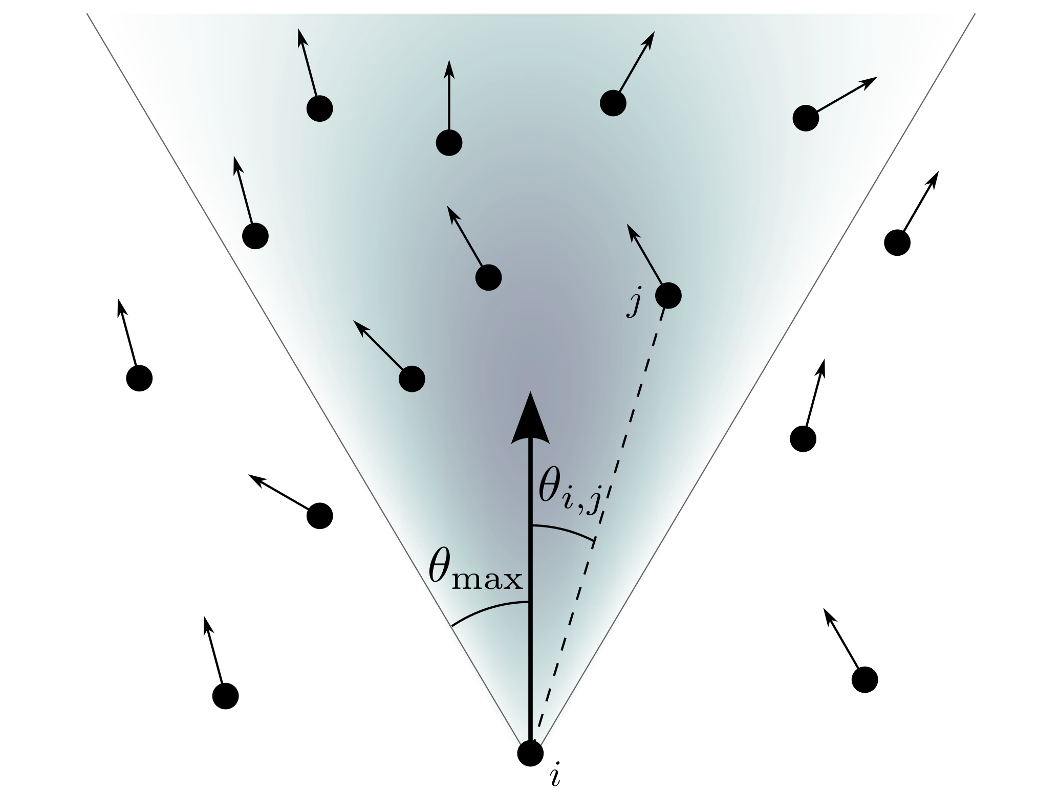
Figure S1: Schematic of the field of view of an agent $i$ that picks an agent $j$ lying within this field of view. The intensity of colour in a given region is related to the the probability with which agent $i$ chooses an agent that lies in that region. Each agent has the highest probability of interacting with agents that lie at a distance $\sigma$ along its direction of motion. Similarly, the intensity reduces as the angle $\theta_{i,j}$ between the velocity of $i$ and the line connecting the agents approaches the maximum bearing angle $\theta_{\rm max}$. Thus, an agent $i$ is most likely to align with an agent that is near its direct line of sight, and which is separated by a distance of around $\sigma$.

Algorithm for computing the number of clusters

At any specified time instant, the maximum possible distance between a pair of agents in the flock is denoted by

$$R_{\max}=\max\left(|\mathbf{x}_{i}(t)-\mathbf{x}_{j}(t)|\right)\,\forall\,i,j\in[1,N]\,.$$

We set the resolution length $R=\lambda\,R_{\max}$ by choosing a value of $\lambda$ in the range $0<\lambda\leq 1$. Each agent $i=1,2,\ldots,N$ is assigned a label $g_{i}$ which is associated with an integer value that specifies the cluster to which the agent belongs to. The cluster-finding algorithm involves determining the number of distinct clusters $N_{c}$ of size $\geq R$. The label of each agent $i$ thus lies in the range $g_{\min}(=1)\leq g_{i}\leq g_{\max}(=N_{c})$.
 
Summary of the variables used:
 
$N$ : Total number of agents in the system, $N_{c}$ : Total number of clusters found using the algorithm, $R$ : Resolution length of the flock (defined above), $g_{i}$ : Label associated with each cluster, $b_{i}$, $c$ : Boolean variables, $g_{\min}$ : Minimum value of the array $g$, $g_{\max}$ : Maximum value of the array $g$.  
 
 
Pseudocode of the algorithm:
 
The algorithm is outlined in the following pseudocode. Comments appear in blue italicised text.

Initalize: $g_{\max}=0$, $g_{\min}=0$, and $g_{i}=0$ for all $i=1,2,\ldots,N$.
For $i=1,2,\ldots,N$
	If agent $i$ has not been assigned a label, we label it as one plus the maximum value of the array $g$.
	If $g_{i}=0$ Then $g_{i}=\max\{g_{i^{\prime}},i^{\prime}=1,2,\ldots,N\}+1$.
	The variable $b$ marks all the agents in the current assignment.
	Initalize: $b_{j}=0$ for all $j=1,2,\ldots,N$.
	Find all agents $j$ that are at a distance $\leq R$ from agent $i$ and assign $j$ with the same label as $i$.
	For $j=1,2,\ldots,N$
		If $|\mathbf{x}_{i}(t)-\mathbf{x}_{j}(t)|<R$ Then
			If $g_{j}=0$ Then $g_{j}=g_{i}$.
			$b_{j}=1$.
		End
	End
	Initalize: $g_{\min}=g_{i}$.
	Consider all the marked agents, i.e. all agents $j$ for which $b_{j}=1$.
	We find the minimum value of $g_{j}$ and assign it to $g_{\min}$
	For $j=1,2,\ldots,N$
		If $b_{j}=1$ Then
			If $g_{j}\leq g_{\min}$ Then $g_{\min}=g_{j}$.
	End
	For $j=1,2,\ldots,N$
		We assign the minimum value of the array $g$ to all the marked agents.
		If $b_{j}=1$ Then
			For $k=1,2,\ldots,N$
				If $g_{k}=g_{j}$ and $k\neq j$ Then $g_{k}=g_{\min}$.
			End
			$g_{j}=g_{\min}$.
		End
	End
End
Compute: $g_{\max}=\max\{g_{i^{\prime}},i^{\prime}=1,2,\ldots,N\}$.
If more than one cluster exists, we relabel them so as to remove the value zero.
If $g_{\max}>1$ Then
	For $i=(g_{\max}-1),~{}(g_{\max}-2),\ldots,1$
		Set: $c=0$
		For $j=1,2,\ldots,N$
			If $g_{j}=i$ Then $c=1$ and Exit.
		End
		Fix gaps in the label numbers to ensure that the final set is contiguous
		If $c=0$ Then
			For $j=1,2,\ldots,N$
				For $k=i+1,\ldots,g_{\max}$
					If $g_{j}=k$ Then $g_{j}=k-1$.
				End
			End
		End
	End
End
Compute: $g_{\min}=\min\{g_{i^{\prime}},i^{\prime}=1,2,\ldots,N\}$, $g_{\max}=\max\{g_{i^{\prime}},i^{\prime}=1,2,\ldots,N\}$.

Once each $g_{i}$ has been relabelled, the number of agents in each cluster $i$ is simply the number of agents that are labelled $g_{i}$, and the total number of clusters at the chosen resolution length $N_{c}=g_{\max}$.
 
Demonstration of cluster-finding algorithm at different resolution lengths:
 
In the following example, we present an implementation of this cluster-finding algorithm at two different resolution lengths, $R$. As displayed in Fig. S2, we consider four clusters of agents. Each cluster consists of $50$ agents whose coordinates are chosen randomly within a $10\times 10$ square centered at the coordinates $(0,0)$, $(0,25)$, $(25,0)$, and $(25/\sqrt{2},25/\sqrt{2})$.

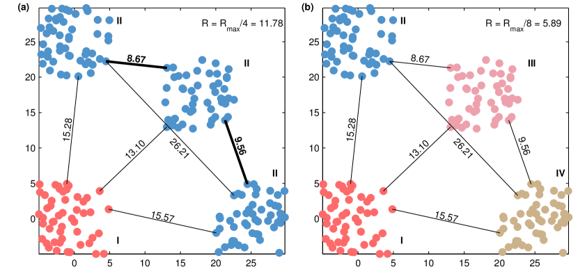
Figure S2: A demonstration of the cluster-finding algorithm. We choose resolution lengths (a) $R=R_{\max}/4$, and (b) $R=R_{\max}/8$. The lines connect the closest agents in each pair of clusters, and the corresponding numerical value denotes the distance between these agents. The bold lines and numbers in panel (a) indicate that the corresponding clusters are categorized as being part of the same cluster (II). In panel (b) four clusters (I-IV) are obtained since all of them are separated by a distance $>R$.

Upon running our cluster-finding algorithm on this flock, we find that the maximum separation between any pair of agents is $R_{\max}=47.13$. For the choices $\lambda=1/4,1/8$, we find $R=R_{\max}/4=11.78$ and $R=R_{\max}/8=5.89$. In the displayed realization (Fig. S2), we find that the minimum distance between agents in the lower left and upper right clusters is $13.1$. Hence, at resolution length $R=11.78$ these two clusters are categorized as being distinct. In contrast the minimum distances between the agents in upper right cluster and those in the remaining clusters are less than $11.78$ and hence they are categorized as being part of the same cluster. Thus, as displayed in Fig. S2(a), at resolution length $R=11.78$ we find just two distinct clusters I & II (coloured red and blue).

For the case where a resolution length $R=R_{\max}/8=5.89$ is used, we find that since all four clusters are separated by a value greater than $R$ they are categorized are being distinct. Thus, our method obtains four distinct clusters (I-IV) at this resolution length, as displayed in Fig. S2(b) where each cluster is coloured distinctly.

Detailed explanation of the nonlinear term in the model

In Eq. (2) of the main text, we introduce a nonlinear term $f(\mathbf{v}_{j}+\mathbf{v}_{i})$, where $\mathbf{v}_{i}$ and $\mathbf{v}_{j}$ are respectively the velocities of agents $i$ and $j$. For the purpose of the current investigation, we consider the functional form $f(\mathbf{v}):=\mathbf{v}(1-|\mathbf{v}|)/(1+|\mathbf{v}|^{\beta})$ with $\beta=3$. Note that if the field of view of agent $i$ is nonempty, i.e. $\Omega_{i}\neq\emptyset$, its velocity at time step $t+1$ is:

$$\mathbf{v}_{i}(t+1)=\mathbf{v}_{i}(t)+\alpha[\mathbf{v}_{j}(t)-\mathbf{v}_{i}(t)+f(\mathbf{v}_{j}(t)+\mathbf{v}_{i}(t))]$$

For the functional form that we consider, we see that $f(\mathbf{v}_{j}+\mathbf{v}_{i})$ vanishes at $|\mathbf{v}_{j}+\mathbf{v}_{i}|=0$, $1$ and infinity, which implies that the velocity $\mathbf{v}_{i}(t+1)\simeq\mathbf{v}_{i}(t)+\alpha(\mathbf{v}_{j}(t)-\mathbf{v}_{i}(t))$ near these values. The case $|\mathbf{v}_{j}+\mathbf{v}_{i}|=0$ corresponds to a situation where the velocities of particles $i$ and $j$ have identical magnitudes and opposite directions. In this scenario, the resulting velocity update effectively prevents a direct collision.

To understand the case $|\mathbf{v}_{j}+\mathbf{v}_{i}|=1$, let us assume that $|\mathbf{v}_{i}+\mathbf{v}_{j}|=1+\epsilon$, where $|\epsilon|\ll 1$. In this situation, we see that

$$f(\mathbf{v}_{i}+\mathbf{v}_{j})=\frac{(\mathbf{v}_{i}+\mathbf{v}_{j})(1-(1+\epsilon))}{1+(1+\epsilon)^{3}}\simeq\frac{-\epsilon(\mathbf{v}_{i}+\mathbf{v}_{j})}{2}\,,$$

Substituting this expression into Eq. (2) of the main text, we find that the acceleration is

$$\mathbf{a}_{i}\simeq\alpha\left(1-\frac{\epsilon}{2}\right)\mathbf{v}_{j}-\alpha\left(1+\frac{\epsilon}{2}\right)\mathbf{v}_{i}\,$$

Using the velocity update expression from Eq. (1) of the main text, we see that $|\mathbf{v}_{i}|_{\epsilon\neq 0}<|\mathbf{v}_{i}|_{\epsilon=0}$ if $\epsilon>0$, and $|\mathbf{v}_{i}|_{\epsilon\neq 0}>|\mathbf{v}_{i}|_{\epsilon=0}$ if $\epsilon<0$. This implies that for $\epsilon>0$, the agent slows down whereas for $\epsilon<0$, it moves faster. In other words, the nonlinear term $f(\mathbf{v}_{j}+\mathbf{v}_{i})$ ensures that the agent’s speed remains close to that of the specified mean value.

Snapshots of flocking patterns observed over range of parameter values

Flocking patterns observed for $\alpha=0.01,0.05,0.1,0.5$, and over a range of $\theta_{\max}$ and $\sigma$, are displayed in Figs. S3–S6.

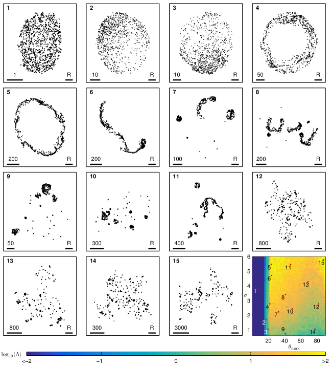
Figure S3: Snapshots of flocking patterns exhibited by the model for a system of $N=10^{3}$ agents, obtained for an interaction strength $\alpha=0.01$, over a range of values of the mean interaction length $\sigma$ and maximum bearing angle $\theta_{\max}$. The corresponding parameter space diagram from the main text is displayed in the bottom right panel. In this panel, we display (in log-scale) the dependence of the average angular momentum of the flock on $\sigma$ and $\theta_{\max}$. Each of the other $15$ panels display flocking patterns observed for parameter values denoted by the corresponding numbered red marker on the parameter space diagram. The numbered solid bars in the lower left corner of these panels provides a measure of spatial distance in each case. The solid bar in the lower right corner of each panel indicates the extent of the corresponding resolution length $R$, which we use for our cluster-finding algorithm.

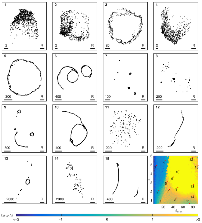
Figure S4: Snapshots of flocking patterns exhibited by the model for a system of $N=10^{3}$ agents, obtained for an interaction strength $\alpha=0.05$, over a range of values of the mean interaction length $\sigma$ and maximum bearing angle $\theta_{\max}$. The corresponding parameter space diagram from the main text is displayed in the bottom right panel. In this panel, we display (in log-scale) the dependence of the average angular momentum of the flock on $\sigma$ and $\theta_{\max}$. Each of the other $15$ panels display flocking patterns observed for parameter values denoted by the corresponding numbered red marker on the parameter space diagram. The numbered solid bars in the lower left corner of these panels provides a measure of spatial distance in each case. The solid bar in the lower right corner of each panel indicates the extent of the corresponding resolution length $R$, which we use for our cluster-finding algorithm.

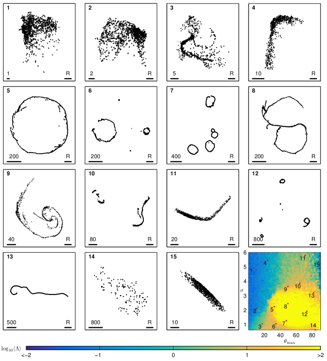
Figure S5: Snapshots of flocking patterns exhibited by the model for a system of $N=10^{3}$ agents, obtained for an interaction strength $\alpha=0.1$, over a range of values of the mean interaction length $\sigma$ and maximum bearing angle $\theta_{\max}$. The corresponding parameter space diagram from the main text is displayed in the bottom right panel. In this panel, we display (in log-scale) the dependence of the average angular momentum of the flock on $\sigma$ and $\theta_{\max}$. Each of the other $15$ panels display flocking patterns observed for parameter values denoted by the corresponding numbered red marker on the parameter space diagram. The numbered solid bars in the lower left corner of these panels provides a measure of spatial distance in each case. The solid bar in the lower right corner of each panel indicates the extent of the corresponding resolution length $R$, which we use for our cluster-finding algorithm.

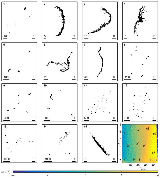
Figure S6: Snapshots of flocking patterns exhibited by the model for a system of $N=10^{3}$ agents, obtained for an interaction strength $\alpha=0.5$, over a range of values of the mean interaction length $\sigma$ and maximum bearing angle $\theta_{\max}$. The corresponding parameter space diagram from the main text is displayed in the bottom right panel. In this panel, we display (in log-scale) the dependence of the average angular momentum of the flock on $\sigma$ and $\theta_{\max}$. Each of the other $15$ panels display flocking patterns observed for parameter values denoted by the corresponding numbered red marker on the parameter space diagram. The numbered solid bars in the lower left corner of these panels provides a measure of spatial distance in each case. The solid bar in the lower right corner of each panel indicates the extent of the corresponding resolution length $R$, which we use for our cluster-finding algorithm. Note that the pattern in panel $1$ is classified as a single cluster because over $90\%$ of the agents belong to that cluster (see algorithm for details). Moreover while the snapshots of patterns in panels $2-4$ may appear reminiscent of the wriggling pattern, their dynamics are in fact qualitatively similar to the meandering pattern.

Description of the movies

The captions for the four movies are displayed below:

• Movie_S1.mp4
  

  Evolution of a system of $N=10^{3}$ agents moving in a wriggling pattern for the case $\sigma=5$, $\theta_{\max}=40$ and $\alpha=0.8$. The system is simulated over $2\times 10^{4}$ time steps, starting from an initial condition where agents are distributed randomly over a small portion of the computational domain. Each frame of the simulation is separated by $50$ time steps.

• Movie_S2.mp4
  

  Evolution of a system of $N=10^{3}$ agents moving in a closed trail for the case $\sigma=3$, $\theta_{\max}=50$ and $\alpha=0.1$. The system is simulated over $2\times 10^{4}$ time steps, starting from an initial condition where agents are distributed randomly over a small portion of the computational domain. Each frame of the simulation is separated by $50$ time steps.

• Movie_S3.mp4
  

  Evolution of a system of $N=10^{3}$ agents moving in a milling pattern for the case $\sigma=1$, $\theta_{\max}=20$ and $\alpha=0.025$. The system is simulated over $2\times 10^{4}$ time steps, starting from an initial condition where agents are distributed randomly over a small portion of the computational domain. Each frame of the simulation is separated by $50$ time steps.

• Movie_S4.mp4
  

  Evolution of a system of $N=10^{3}$ agents moving in a flock with a meandering center of mass for the case $\sigma=3$, $\theta_{\max}=15$ and $\alpha=0.02$. The system is simulated over $2\times 10^{4}$ time steps, starting from an initial condition where agents are distributed randomly over a small portion of the computational domain. Each frame of the simulation is separated by $50$ time steps.