GPU-Accelerated Simulations of Isolated Black Holes

Abstract

We present a port of the numerical relativity code SpEC which is capable of running on NVIDIA GPUs. Since this code must be maintained in parallel with SpEC itself, a primary design consideration is to perform as few explicit code changes as possible. We therefore rely on a hierarchy of automated porting strategies. At the highest level we use TLoops, a C++ library of our design, to automatically emit CUDA code equivalent to tensorial expressions written into C++ source using a syntax similar to analytic calculation. Next, we trace out and cache explicit matrix representations of the numerous linear transformations in the SpEC code, which allows these to be performed on the GPU using pre-existing matrix-multiplication libraries. We port the few remaining important modules by hand. In this paper we detail the specifics of our port, and present benchmarks of it simulating isolated black hole spacetimes on several generations of NVIDIA GPU.

1 Introduction

Numerical relativity (NR), the direct numerical integration of the Einstein field equations, is now a mature subfield of computational physics, with stable binary black hole evolutions possible since 2005 [1, 2, 3, 4, 5]. Binary black hole NR is of central importance for gravitational waveform modeling. For instance, the SpEC waveform catalogues [6, 7] were used in the development of EOB-waveform models [8, 9, 10]. Waveform models calibrated to numerical relativity were used to analyse the resent BBH gravitational wave events detected by LIGO and Virgo [11, 12]. Furthermore, NR binary black hole simulations were used to assess systematic errors of parameter estimation of these GW events [13, 14, 15].

Detailed knowledge of expected waveforms, themselves coming ultimately from NR simulations, are required by these detectors to maximize sensitivities, to interpret observation, and to make tests of general relativity [16]. Ground based detectors’ relative insensitivity to e.g. eccentric binaries is, conversely, in part due to a lack of production-quality simulations in the eccentric region of parameter space [17], a situation which also impairs comparisons with analytic theory.

The intricacy of the Einstein equations presents two challenges to NR. First, interesting simulations are expensive, with wallclock times measured in weeks or months. Second, codes able to perform such simulations are quite intricate from a software engineering perspective. Applying them to new regions of the binary black hole parameter space - let alone to new spacetimes - can require months of effort by small groups of experts. These issues are difficult to address simultaneously, since improving runtime tends to complicate code, and vice versa.

Twenty years ago, the simplest solution would have been to simply wait for hardware to improve. Unfortunately CPU clock frequencies have been essentially static for some time now, with new high-performance computers instead employing increasingly massive levels of parallelism. But few codes scale to $100000$s of CPUs without considerable reformulation.

Easier speedups can sometimes be achieved using “accelerated” architectures. A popular choice is the Graphics Processing Unit (GPU). Problems in graphical computation might involve, for example, computing pixel states as a virtual object moves three-dimensionally. Each pixel is data independent, and the fundamental operations are linear transformations such as rotations. Thus, viewed more abstractly than perhaps originally intended, GPUs are optimized for highly parallelizable linear operations. These are performed by slow, but numerous and tightly-coupled, processors connected by various hierarchies of memory. The tight coupling and fast RAM make intra-GPU communication inexpensive. Because of this, GPUs are, for suitable problems, potentially dramatically superior to CPUs in terms of e.g. FLOPS-per-watt.

The extra parallel cores replace the CPU’s extensive control circuitry, which for example rearranges instructions to optimize single-thread performance, along with much of its cache memory, which increases the speed of non-contiguous memory access. GPUs are thus less flexible than CPUs, and less able to handle fundamentally serial problems. But even for less-than-ideal use-cases, GPUs have a major advantage over CPUs: they continue to demonstrate Moore’s-law-like FLOPS/year scaling with new releases. Therefore, once the initial investment is made to produce a port, further speedups can be made by simply buying new hardware.

GPUs now enjoy widespread and increasing use as “accelerators” of numerically-intensive, linear-algebra-heavy tasks such as physical simulation and deep machine-learning. At the time of writing, they have not been widely adopted in NR, due likely to the complexity introduced by the low-level nature of GPU coding. Some previous applications of GPU computing to NR do, however, exist. Zink [18] used a CUDA-based finite-difference code to evolve a gauge wave upon Minkowski spacetime. Later, he developed HORIZON [19], a GPU-accelerated GRMHD code. Yang et al. [20] simulated plunging black-hole binaries in the BSSN formalism using a finite-difference CUDA port of the numerical relativity code AMSS-NCKU [21, 22]in concert with an AMR-like algorithm of their own design. Chen [23] used a GPU-accelerated approach to solve sample coupled elliptic equations using the spectral collocation and spectral Galerkin methods. The Teukolsky master equations [24] describing perturbations to the Kerr spacetime have been solved using the Cell processor SDK [25], OpenCL [26, 27], and CUDA [28]. Herrmann et. al [29] used CUDA to integrate the PN equations at an unspecified truncation order. Brugmann [30] developed a GPU algorithm to integrate PDE systems relating time-dependent tensor fields on a spherical shell using pseudospectral methods. Perhaps most similarly to our work, automatically-generated GPU code has been used to benchmark binary black holes inspirals simulated using the Einstein Toolkit [31].

In the present work we describe our approach to the GPU porting of a specific NR code, the Spectral Einstein Code ($\mathtt{SpEC}$) [32]. Multi-domain spectral methods like those used by $\mathtt{SpEC}$ solve PDEs by dividing the simulation volume into “domains” upon which the solution is smooth. Within each domain, the solution can then be represented as weights to a truncated sum of basis functions. Data thus represented are nonlocal in space. Every processor working on the same domain will generally require access to the full spectrum.

$\mathtt{SpEC}$ already uses MPI to assign each domain to a different processor. In setups where multiple CPU cores share RAM, it should also be possible to assign multiple cores to a single domain, but this has not been achieved in practice despite repeated efforts. On the other hand, the many processors within a single GPU also share a unified pool of memory. Access to this memory is sufficiently fast that the entire GPU can work on the same domain. GPUs, in other words, enable $\mathtt{SpEC}$ to scale to higher levels of parallelism than would be otherwise possible. Conversely, $\mathtt{SpEC}$’s inability to utilize OpenMP means that the relevant benchmark in this work is the performance of a single CPU to an entire GPU.

In principle the Einstein equations are merely a specific example of a hyperbolic PDE system to be solved, which presents challenges on either the CPU or GPU identical to any other. The algorithmic reasoning employed in this work is indeed quite straightforward, and our challenges have instead been more practical. In simple terms, the $\mathtt{SpEC}$ source code is very long and complicated. Computational effort is spent mostly on a relatively small number of modules, but in practice these are each implemented by a complex and diverse set of subclasses depending on, for example, the topology of the domain (cubes, cylinders, spherical shells, etc.) upon which they operate.

Producing GPU equivalents of all the necessary instances would involve considerable effort. More problematically, upon completion code maintenance would become infeasibly difficult, since consistency between the CPU and GPU code bases would have to be continuously maintained at each revision. Of course, only relatively little code is actually performance-critical enough to yield practical benefits from GPU acceleration. Porting only these critical segments, however, results in numerous expensive CPU-GPU memory synchronizations, since the input to and output from the critical modules must be accessible to the relevant processor. This expense swamps any speedup in practice.

To keep the amount of redundant code manageable, we use a combination of porting strategies relying upon various levels of automation. At the highest level of automation, we have developed a C++ library, TLoops, which provides technology to write spatially-decoupled tensor-algebraic expressions directly into C++ source code. For example, the TLoops expression of listing 1 yields output equivalent to that of listing 2.

Listing 1: Example TLoops expression.

⬇

Tensor<DataMesh> dtg, K, db;

DataMesh alpha;

// initialize dtg, K, db, alpha

dtg(Sym<0,1>(),i_,j_)=-2*alpha*K(i_,j_)+db(i_,j_)+db(j_,i_);

Listing 2: C-style code, equivalent to Listing 1.

⬇

Tensor<DataMesh> dtg, K, db;

DataMesh alpha;

// initialize dtg, K, db, alpha

for(int i=0; i<3; ++i) {

for(int j=0; j<=i; ++j) {

for(int a=0; a<N; ++a) {

dtg(i,j)[a]=-2.0*alpha[a]*K(i,j)[a]+db(i,j)[a]+db(j,i)[a];

}

}

}

Here DataMesh is SpEC’s array class, representing one double precision value at each point on a simulation domain, while Tensor<DataMesh> is a container class representing one DataMesh for each component of a tensor (field). TLoops can run the code in Listing 1 at once, or can output equivalent GPU code to be linked against a separate SpEC compilation, allowing for efficient GPU porting with very minimal effort (the replacement of code in the form of Listing 2 with TLoops expressions such as those of Listing 1). TLoops will also output equivalent GPU code to the line inside the loop in Listing 2, allowing almost the entire SpEC code to be (inefficiently) ported at once.

TLoops, thus, allows SpEC to keep data always on the GPU without any additional coding. Code segments which consume large amounts of wallclock time and which consist mostly of tensor manipulations, such as the code SpEC uses to advance the Einstein equations in their generalized harmonic formulation by a timestep, can usually be sped up by at least 10 times relative to the GPU through the use of TLoops statements such as Listing 1.

At the next levels of automation, there are a number of modules that are performance-critical, but which cannot be handled by TLoops because they are not spatially-decoupled (i.e. their output at a given gridpoint depends on simulation data at other gridpoints). These modules, which include the differentiator for example, turn out to have several key features in common. First, each may represent any of various transformations, and often multiple implementations of each. The differentiator, for example, may be handled using a matrix multiplication, or by spectral methods whose details depend on the domain topology, with the choice being made by the user at runtime. The number of possible execution branches is too large to port everything by hand.

Fortunately, all such modules used by SpEC turn out to represent linear transformations whose matrix representations have finite rank. Furthermore, while the number of possible execution branches is very large, the number of actual branches encountered by a particular process is in practice manageably small. We therefore write GPU code which implements finite linear transformations, given an explicit matrix representation of them. In this way many lines of code may be ported with relatively little effort.

There are, finally, some modules which are neither amenable to TLoops nor to the cached linear transformation approach. This last class includes, for example, sequences of contractions with Jacobian matrices designed to transform the spatial coordinates of a spacetime tensor while leaving the temporal coordinates unchanged. These are few enough to simply port by hand.

In concert, thus, our strategy consists first of automated porting of existing expressions using TLoops, with the loops in some especially important modules replaced by TLoops expressions. Next, we port linear transformations by tracing out their explicit matrix representation, and port the few remaining important segments by hand.

The rest of this paper is structured as follows. Section 2 describes $\mathtt{SpEC}$ and introduces the GPU architecture. Section 3 gives a detailed, module-by-module description of our port including benchmarks. Section 4 presents and discusses holistic benchmarks of the entire SingleBH test case. Finally, Section 5 draws conclusions and motivates future research.

2 Background

2.1 The Spectral Einstein Code

The Spectral Einstein Code ($\mathtt{SpEC}$) [32] is a C++ code designed to solve Einstein’s equations of general relativity. Its primary purpose is to simulate inspiraling and colliding black holes and neutron stars.

For a binary black hole spacetime, $\mathtt{SpEC}$ employs a domain-decomposition, dividing the computational domain into about 60 elements, or “domains”. Different domains may have different shapes, such as cubes, cylinders, and spheres. These may in turn have different connectivity and consequently different spectral basis-functions. In this paper, we only consider single black hole spacetimes, where the domain-decomposition consists of a set of concentric spherical shells.

$\mathtt{SpEC}$ employs the method of lines to evolve collocation point values of about 50 fundamental variables using a high-order Dormand Prince timestepper [33]. Non-linear terms such as those in the Einstein equations are directly computed at the collocation points.

Derivatives, filtering, and interpolation are performed using spectral transforms. First, the collocation data is transformed to the appropriate spectral space. Derivatives and filtering are then implemented as operations on the spectral coefficients. The result is transformed back to collocation space.

The evolved variables are tensorial, e.g. $\psi_{ab}(x^{i})$. Here, $a,b=0,1,2,3$, indicate space-time components, and $x^{i}$ are the spatial coordinates. Some operations, like the computation of derivatives, operate on each tensor-component separately. Others couple different tensor-components. For instance, filtering in a spherical shell relies on a representation of data in terms of tensor spherical harmonics, to achieve a consistent truncation of components in angular resolution.

$\mathtt{SpEC}$ employs the dual-frame approach [34]. Here, data is represented at collocation points at fixed grid-coordinates, the coordinate system in which the domain-decomposition is specified. The evolution equations, however, are formulated in asymptotic inertial coordinates. The two coordinate systems share the same time-coordinate, and their spatial coordinates are related by a time-dependent coordinate transformation.

$\mathtt{SpEC}$ is a highly configurable code. Many modules are defined through abstract base-classes, and are implemented in derived classes. The concrete derived classes to be used for a certain domain can be chosen at runtime through parameter files. These choices include the coordinate mappings between simulation and output coordinates, which filters to implement, and how spectral transformations are performed (e.g. via FFTs or via a BLAS-matrix call), and how interpolation is performed (via a direct summation of the spectral series, or via a FFT onto a finer grid followed by polynomial interpolation). This configurability leads to many execution paths through a program.

2.2 Programming for NVIDIA GPUs

Here we briefly introduce the pertinent characteristics of the GPU architecture [35, 36, 37, 38, 39], as it compares with the more familiar CPU architecture. The CPU employs a small number ($1$-$4$ in the diagram, and up to several $10$s in contemporary examples) of cores that perform actual computations. All memory is accessible by all cores. Some, much faster, memory is used to cache data on the grounds that repeated accesses are likely. This caching is not managed explicitly by the user at the software level.

A relatively large amount of space is devoted to control circuitry, which for example performs hardware-level optimizations. The extensive control circuity, transparent memory caching, low levels of parallelism, and fast serial performance give the CPU great flexibility to handle a wide variety of problems. Partly because of this flexibility, and partly because serial programs are much easier to optimize at the compiler level, it is rare that a developer need think about the hardware when writing code.

The idea of the GPU is essentially to gut this entire structure and replace it with as many processing cores as possible. All such cores are connected to a pool of “global” memory, which is relatively slow, though still faster than CPU memory. A very small global memory “L2” cache may be present, but it is in practice negligible compared to the CPU cache. Programmers must thus carefully manage the manner in which global memory is accessed to achieve reasonable levels of performance, especially since the speed of global memory access is very often the limiting performance factor.

The cores are organized into groups called streaming multiprocessors (SMs). Each SM (pairs of SMs in some architectures) houses a small amount of control circuitry and a hierarchy of much faster memory pools available only to it. These include another small cache, a pool of fast “shared” memory, and a number of very fast registers. A thread scheduler delegates processes to individual SMs.

Each SM has an independent control-logic, shared by all cores within each. This saves dye-space, but means that all cores in an SM execute instructions in lockstep. Each core may, however, execute these instructions upon a different global memory address. GPUs are therefore designed to implement the SIMD (Single Instruction, Multiple Data) model of parallelism. Programmers must take care to avoid conditional statements which make the instructions executed by individual cores dependent upon their individual data. Such statements cause the entire SM to execute each branch of the conditional in serial.

For most of their history GPUs could be programmed only via heavily graphically-oriented “shader” languages. Much more flexible access is now possible via generalized GPU frameworks such as NVIDIA’s own CUDA [40]. CUDA allows the GPU to be manipulated through a low-level C-like interface. Parallelism is abstracted as a hierarchy of logical structures adapted for execution by the physical structures described above.

These logical structures derive their names from an inconsistent and confusing metaphor with looms. Instructions are given to the GPU by writing a CUDA kernel, which is roughly analogous to a C function. Typically, a kernel reads an array from global memory, performs some computation, then stores the results back in global memory. When executing a kernel, the programmer assigns a number of blocks, and to each block a number of threads. Blocks are always local to an SM and may therefore exploit SM-local resources such as shared memory. Each individual thread, which has a unique index, serially executes the instructions in the kernel. The thread index can be used to address global memory, and in this way operations on arrays can be parallelized.

When the kernel is executed, the thread scheduler assigns the blocks to individual SMs. The blocks are then divided into groups of 32 threads called warps, which execute instructions in lockstep. Each SM can simultaneously execute multiple warps, with the exact number depending on the specific GPU architecture. This allows SMs to hide latency: while an instruction in a particular warp e.g. waits for data, the SM may execute instructions from another warp rather than simply idling.

Writing efficient CUDA code requires low-level awareness of hardware. The most serious performance issue comes from the fact that the CPU and GPU have physically different memory. Any data the GPU (CPU) needs from the CPU (GPU), including the kernel machine code itself, must be transferred over an interconnect. Such transfers must be kept to a minimum: both in size, since CPU-GPU interconnects are slow, and in number, since initiating a new transfer carries significant latency, and since all potentially-asynchronous GPU operations must be halted while memory is modified.

The necessity of reasoning explicitly about the low level details of memory access accounts for much of GPU programming’s difficult reputation. A warp always accesses global memory contiguously as a unit. Anything other than contiguous accesses in groups of 32 entries requires that the entire warp make multiple accesses. The shared memory and registers localized within streaming multiprocessors permit comparatively fast random access, so data can be cached here after a contiguous access to global memory. But this must be done manually by the programmer, and the use of shared memory in particular can easily create e.g. race-conditions. The explicit synchronizations required to manage these, and the rather cryptic error messages supplied by CUDA when such management has been done improperly, can greatly complexify kernels.

At the kernel level the most important optimizations stem from two essential differences between the CPU and the GPU. First, GPUs suffer considerable single-thread latency. However, these latencies can potentially be hidden by asynchronous execution. Ideally, then, kernels and blocks should execute for times much longer than their scheduling overhead. They should also be numerous enough that all SMs are constantly occupied (but see [41]), which also helps to hide any remaining latency. Blocks should finally have threadsizes which are multiples of 32 (the number of threads in a warp), since warps are indivisible and otherwise some cores will be left idle.

Second, compared to the CPU, the GPU performs (parallel) computations far more quickly than memory accesses. A GPU-friendly algorithm should ideally be compute-bound, meaning that its arithmetic intensity, or ratio of computations to memory accesses, is sufficiently high that the algorithm becomes faster with increased computational power, rather than memory speed. In the opposite situation of a memory-bound kernel, speedup will be limited by the bandwidth of the GPU memory. This will be an important consideration when analyzing the performance of our implementations.

2.3 GPU Benchmarking

Throughout this study we will often be concerned with the actual performance achieved by GPU implementations of some algorithm compared with what is theoretically possible. We will also be concerned with the advantage achieved by the GPU, relative to the CPU, when used with hardware that is realistically available to SpEC users. In this subsection we lay out our general approach to benchmarking, and thus to quantification of such notions.

We first estimate the potential performance of each algorithm according to the following (rather well-established) framework. We view each algorithm as consisting first of $M$ memory transactions, i.e. loads and stores of size $w$ bytes to and from RAM, resulting in $D=10^{-9}wM$ GB of data transacted total. All operations in this study are in double precision and we take $w$ to be $8$ bytes throughout. The algorithm also performs $F$ floating-point operations - multiplications and additions - a term we loosely identify with “instructions”, and which we measure in GFLOPs. Such an algorithm can be characterized by its arithmetic intensity $I$

$$I\equiv\frac{F}{M}$$ (1)

which, since GFLOPs are just numbers, is dimensionless.

These $D$ and $F$ are what we estimate to be the minimum possible amounts of transacted data and floating-point operations that any implementation of a given algorithm must perform. We suppose that, if run on hardware which can process data at an optimal bandwidth of $B$ GB/s and an optimal processing power of $P$ GFLOP/s, an algorithm will ideally spend $D/B$ seconds on memory transactions and $F/P$ seconds on floating-point operations. Assuming all latency can be hidden, the total execution time would be $T=D/B+F/P$. Considering two devices $i$ and $j$ with performance characteristics $B_{i},P_{i}$ and $B_{j},P_{j}$, respectively, the potential speedup from device $j$ over device $i$ is

$$\mathrm{speedup}=\frac{T_{i}}{T_{j}}=\left(\frac{wB_{i}^{-1}+IP_{i}^{-1}}{wB_{j}^{-1}+IP_{j}^{-1}}\right).$$ (2)

This also assumes that an implementation which minimizes $M$ and $F$ has been achieved on both devices.

When $I=I_{\mathrm{eq}}\equiv wP/B$, a processor will spend equal amounts of time on memory operations and arithmetic. Put differently, an algorithmic redesign that makes unnecessary the transmission of $D_{-}$ GB of data by performing $F_{+}$ extra GFLOPs will be an optimization when $F_{+}<I_{\mathrm{eq}}D_{-}$. We therefore consider an algorithm to be “memory” rather than “compute” bound when $I<I_{\mathrm{eq}}$.

Depending on whether we expect algorithms to be memory or compute bound, we present benchmarks in terms of one of two quantities: the effective bandwidth $BW_{\mathrm{eff}}$, measured in GB/s or the effective processing rate $P_{\mathrm{eff}}$, measured in GFLOP/s. Given the actual measured time $t$ required to perform the benchmarked operation, these are defined by

$$\mathrm{BW}_{\mathrm{eff}} \equiv\frac{D}{t},$$ (3)

$$P_{\mathrm{eff}} \equiv\frac{F}{t}.$$ (4)

For algorithms which are heavily memory or compute bound, these quantities will be comparable to and bound from above by $B$ and $P$ for a given device, which allows for quick characterization of the achieved performance. More precisely, we can compute theoretically optimal performance metrics as

$$\mathrm{BW}_{\mathrm{eff,opt}}=w\frac{BP}{wP+IB}$$ (5)

$$P_{\mathrm{eff,opt}}=I\frac{BP}{wP+IB}.$$ (6)

Observed performance far beneath these values indicates that further attention to optimization may be worthwhile: the algorithm as writen may, for example, be performing extraneous operations or spending excessive time on latency.

Table 1 shows the vendor-reported $B$ and $P$ along with an actual measured value for $B$ obtained by running the CUDA SDK program bandwidthTest, which simply times the result of a device-to-device memory transfer. Using these measured figures we also compute $I_{\mathrm{eq}}$ for each of four devices: a single core of an Intel Xeon E5-2620 CPU, along with M2090, K80, and P100 GPUs. We use a single CPU core because, as discussed earlier, SpEC is incapable of OpenMP-style parallelization of work upon a single domain across CPU cores. In Figure 1 we furthermore display $\mathrm{BW}_{\mathrm{eff}}$ and $P_{\mathrm{eff}}$ for each processor. We also plot the “speedup”, i.e. the ratio between the execution time on one of the GPUs from Table 1 with that of the CPU. Larger speedups indicate better GPU-than-CPU performance. We will be interested in this quantity (computed using the actually measured execution times) throughout this study.

These figures allow us to draw two immediate conclusions. First, the theoretical speedups range between about 4 and 400, which given that NR runtimes are typically measured in weeks or months represents a dramatic increase in productivity even in the pessimistic case. Note that actually achieved speedups may in fact be higher than “optimal”, since the CPU algorithm may not be fully optimized, since one will typically rewrite an algorithm to achieve a more favourable value of $I$ during a port, and since latency may not affect all processors equally in practice. Second, realizing such speedups requires high values of $I$, to a much greater or even opposite degree as would be optimal on the CPU, as demonstrated by the approximately linear dependence of speedup upon $I$ between $I$ of around $1$ to $100$. Effective porting thus often requires implementations, and sometimes whole algorithms, to be redesigned in order to minimize memory transactions relative to floating-point operations.

	B		P	$I_{\mathrm{eq}}$
Device	theoretical, GB/s	measured, GB/s	GFLOP/s
CPU	42.7	-	8.0	0.41
M2090	177.6	123	665.5	5.41
K80 (one card)	280	170	932–1456	5.48–8.56
P100	720	449	4036-4670	9.0–10.4

Table 1: Performance specifications for our benchmarked processors. The columns are defined during the discussion in Section 2.3. “CPU” refers to a single core of an Intel Xeon (Sandy Bridge) E5-2620. The K80 actually contains two separate GPUs (which share memory) on the same card. Using both requires similar extra effort as multi-GPU programming generally, so we profile only one throughout. The K80 and P100 are also potentially capable of “GPU Boost”, which dynamically adjusts the core clock frequency if it is possible to do so without exceeding thermal and power limits (the CPU has similar capabilities). The “measured” bandwidths were obtained by running the CUDA sample program bandwidthTest.

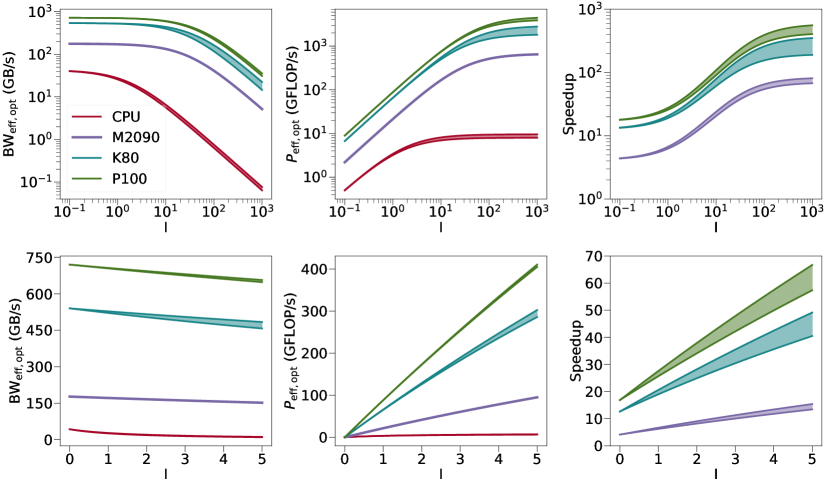
Figure 1: Top Panels: Effective bandwidth, processing rate, and theoretical speedup vs. a single core of the Intel Xeon E5-2620 as a function of arithmetic intensity in double precision for the three GPUs we benchmark in this study. Improvements to arithmetic intensity are critical around $I=1-100$, when the speedup dependence is nearly linear. This assumes zero latency on both CPU and GPU, and that the algorithm running on both be exactly identical; neither assumption will hold in practice. The ranges account for the dynamical clock frequencies of all devices except the M2090. Bottom Panels: Zoom-ins around $I=0$ to $5$, relevant to the Jacobian contractions benchmarked later.

In Figure 2 we, as an example, show benchmarking information collected from the P100 GPU performing the DiffJac operation described in Section 3.3. We measure performance by $\mathrm{BW}_{\mathrm{eff}}$, computed from Eq. (3). This equation requires an estimate of the logical size of the operation $D$, which for us is just $8$ bytes multiplied by $M$, computed also in Section 3.3. Higher values of $\mathrm{BW}_{\mathrm{eff}}$ indicate better performance. We consider performance to be “good” when it is “near” the estimated optimal performance $\mathrm{BW}_{\mathrm{eff,opt}}$ calculated from Eq. (5), and plotted in Figure 1.

Eq. (5) involves $I$ and thus both $M$ and $F$. Therefore, our benchmark presentations will usually take the following form. First, we will introduce the operation to be benchmarked, describing what it does and how we have ported it. Next, we will construct a model to estimate $M$, $F$, and $I$. Based on whether $I$ is typically less or greater than the values of $I_{\mathrm{eq}}$ for the GPUs in Table 1, we will present plots of either $\mathrm{BW}_{\mathrm{eff}}$ (when $I<I_{\mathrm{eq}}$, so that performance is bound most strongly by memory bandwidth) or of $P_{\mathrm{eff}}$ (when $I>I_{\mathrm{eq}}$, so that performance is bound most strongly by processing power). In either case, larger values indicate better performance. We will then discuss these plots, paying special attention to how closely the observed performance matches the ideal performance: either $\mathrm{BW}_{\mathrm{eff,opt}}$ or $P_{\mathrm{eff,opt}}$.

The machines we had access to for our K80 and P100 tests are head nodes, whose operating systems do not employ batched processing. As a result our benchmarks in these cases are much noisier than for the M2090 and CPU tests. We presume the noise to be due to machine resources being assigned to processes besides those we seek to time. To correct for this we run each test 50 separate times. The individual benchmarks show an obvious trend contaminated by rare, but extreme, dips in performance that do not persist across runs. We thus take, at each gridsize, the median result of the 50 runs. To illustrate this, Figure 2 plots 10 individual benchmarks from the DiffJac operation described in Section 3.3, with the median overlaid on top. The individual benchmarks mostly agree apart from isolated large spikes. The median tracks the agreement.

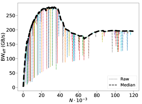
Figure 2: Individual raw benchmarks from the DiffJac operation (dotted coloured lines) on the P100 operating on $T_{abb}$. The median at each gridsize, which clearly tracks the overall trend, is overlaid as a dashed black line.

3 Details of our port

3.1 Overview

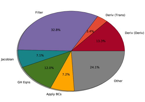
Figure 3: Illustration of the relative importance of the modules encountered by SpEC during simulation of an isolated black hole.

We now turn our attention to SpEC-based black hole simulations. The case we consider throughout is the evolution of a single black hole. This avoids additional complexities that occur for binaries, most notably apparent horizon finding and MPI. This evolves analytically-computed Kerr-Schild initial data for an isolated black hole, defined by its mass $m$ and its dimensionless spin-vector $\vec{\chi}$. For a black hole with mass $m$ and angular momentum $\vec{J}$, one defines this dimensionless spin-vector as

$$\vec{\chi}=\frac{c}{G}\frac{\vec{J}}{m^{2}}.$$ (7)

Black holes must have $0\leq|\vec{\chi}|\leq 1$. For our test, we choose $\vec{\chi}=(0.2,0.3,0.4)$, representing a moderately spinning black hole whose spin axis is not aligned with any of the coordinate axes.

The spectral domains are two nested spherical shells centred on the hole, the first extending radially from $r=1.62m$ to $r=6m$ and the second from $r=6m$ to $r=12m$. This is sufficient for the simulation to remain stable for at least several thousand timesteps. A full BBH simulation would involve domains besides spherical shells, but spherical shells are the most important, the most individually expensive, and the least friendly to GPU acceleration. The spherical shells in this simulation have 10, 19, and 38 points respectively along their radial, polar, and azimuthal coordinates, for a total gridsize of 7220 points. We profile throughout from the 5th to the 105th timestep to avoid contamination by simulation setup costs, which are negligible in production runs.

The pie chart of Figure 3 illustrates, by percentage, the per-module compute time spent by $\mathtt{SpEC}$ during such a simulation at a resolution comparable to that of a binary production run. These modules do the following:

1. Jacobian - contracts the spatial components of a tensor with a Jacobian as part of a coordinate transformation.

2. Deriv - computes the gradient of a tensor (‘Deriv’). This is followed by another Jacobian multiplication (‘Trans’).

3. Filter - maps from physical to spectral space, applies a filter function, and maps back.

4. GHEqns - Computes the right-hand side of the Einstein equations.

5. Apply BCs - extracts the two-dimensional data at the boundaries of the domains, applies the boundary conditions to these, and inserts them back into the three-dimensional volume data.

6. Other - all other operations, each individually negligible.

The rest of this section presents our approach to porting (or justifies leaving unported) each of these.

3.2 Memory Management

The physically separate memory of the CPU and GPU mean that data must be kept synchronized between the two devices: accesses to arrays in CPU memory must have a means to ensure that they have not been made obsolete by a computation upon their GPU counterparts, and vice versa. Since the actual synchronizations are very expensive, we would like to perform them only when actually necessary. Normally this is handled explicitly by the user, but this approach would in our case require an excessive number of API calls. We have instead developed C++ classes to “lazily” hide memory management from the user. Two arrays are maintained, one on each device, with allocations or copies made only when necessary.

It turns out that GPU memory allocation is extremely expensive. Since SpEC unfortunately makes many allocations and deallocations of memory, the naiive approach of allocating and deallocating GPU memory in turn can massively degrade performance. On the other hand it is clear that repeated allocations will be typically redundant. If an array of a given size is allocated at one timestep, another array of the same size will very likely be allocated at the next timestep as well.

It therefore becomes advantageous to cache rather than deallocate GPU pointers upon array destruction. We handle this memory cache with a rather straightforward map that keeps a list of pointers to allocated, but presently unused, GPU-memory. Initially, this cache is empty. Any GPU memory allocation first checks the cache for an available portion of already-allocated GPU memory. A pointer to such a portion, if found, is removed from the cache, and returned to the user-code. If no allocation is found, a new one is made using the usual CUDA library call.

When a portion of GPU-memory is no longer needed by the code, we do not fully deallocate the memory via a CUDA library call. Instead, we simply add the pointer to the memory cache, to be reused when the next time a memory segment of this size is requested. We monitor overall GPU memory usage; true deallocation occurs when the total allocated memory exceeds a certain size, or when explicitly performed by the user. The inspiration for this approach is from [42], although our implementation is very simplistic, being based on C++ standard library containers.

Usually, our array class $\mathtt{DataMesh}$ does not occur alone, but as an element within our container class Tensor. Tensor handles indexing in such a way as to represent a mathematical tensor with a given dimension, rank, and symmetry structure. Quite often, $\mathtt{SpEC}$ will perform some operation uniformly on all elements of a Tensor. Due to the kernel launch overhead GPU, it is much more efficient to handle the entire Tensor at once than it is to launch a new kernel for each individual $\mathtt{DataMesh}$.

$\mathtt{SpEC}$, however, allows the elements of a Tensor to be of arbitrary type, and does not assume they have a uniform memory layout. This is achieved by handling Tensors as arrays of pointers, one per element, which have no relationship to one another in linear memory. On the CPU this is usually not a problem: calling a function once per tensor element is essentially free, as is iterating through the Tensor. But on the GPU calling one kernel per element is quite expensive. A single kernel could process the entire Tensor, but to do so the list of pointer-to-elements would need to be copied to the GPU, and this copy carries again a large amount of overhead.

In practice, the capability of Tensors to store nonuniform objects is rarely used, so we handle this situation with a compromise. Each Tensor stores a list of “GPUPointers”, which is initially empty. When the GPUPointers are explicitly asked for, they are constructed on the host and synchronized with the device. Subsequent accesses to the GPUPointers first check whether the Tensor has been reshaped and synchronize again only if it has. This means that if the same Tensor is accessed multiple times during a timestep (which often happens), the GPUPointers will be synchronized only once.

3.3 Jacobian multiplication

$\mathtt{SpEC}$ includes two performance-critical modules implementing coordinate changes as contractions with a Jacobian matrix. The first, which we call “DiffJac”, occurs after differentiation, bringing the derivative index into the same coordinate frame as the tensor indices. Indices $(a,b\ldots)$ run over spacetime and $(i,j\ldots)$ over space, while we represent partial differentiation with a comma. Then this operation may be written symbolically as

$$T\indices{{}_{ab\ldots,i}}=J\indices{{}_{i}^{j}}T\indices{{}_{ab\ldots,j}},$$ (8)

where $T\indices{{}_{ab\ldots,i}}$ is the tensor being transformed and $J\indices{{}_{i}^{j}}$ is the Jacobian of the transformation. The code does not distinguish between contravariant and covariant indices; we do so here only to clarify which indices are being summed over.

The second operation, which we call “SpatialCoordJac”, makes a coordinate change of a tensor’s spatial indices only, by contracting every possible combination of said spatial indices with the Jacobian. First, one contraction per rank is performed over the purely spatial indices. Next, each index is respectively set to its timelike component and one contraction per remaining index is performed. Subsequently, two indices are made timelike, followed by contractions over all unfixed indices, etc. In the case of a rank 2 tensor $T_{ab}$, for example, this operation may be written

$$T_{ij} =J\indices{{}_{i}^{k}}J\indices{{}_{j}^{l}}T_{kl},$$ (9)

$$T_{0j} =J\indices{{}_{j}^{l}}T_{0l},$$ (10)

$$T_{i0} =J\indices{{}_{i}^{k}}T_{k0}.$$ (11)

The purely timelike component encounters a null-op, having been “contracted with no Jacobians”.

In practice, both of these operations are only ever applied to tensors with the following four rank and symmetry structures: $T_{a}$, $T_{ab}$, $T_{aa}$, $T_{abb}$. The subscripts on the above represent the rank and symmetry structure of the tensor $T$, with repeated indices indicating a symmetry. Thus $T_{abb}$ indicates a dimension 4, rank 3 tensor satisfying $T_{abc}=T_{acb}$. In the case that a symmetry structure other than one of those specified above is encountered, our port falls back on the CPU code.

The actual kernels are fairly simple. They could likely be optimized further, but already perform sufficiently well that Jacobian multiplication is a very small expense on the GPU. For the DiffJac operation of Eq. (8), we first copy the pointer addresses of the individual tensor elements into linear GPU arrays. We divide the CUDA grid into two-dimension thread-blocks. The x-coordinate runs over the spatial grid, the block index of the y-coordinate labels the components of the input tensor, and the thread index of the y-coordinate those of the Jacobian. Each block therefore has local to it all the Jacobian tensor pointers necessary for the contraction, which we load into shared memory to limit register consumption. Each thread performs the contraction in serial.

The SpatialCoordJac operation of Eqs. (9)-(11) proceeds similarly. Rather than copying individual tensor indices into a GPU array, we bundle them into a struct which is sent to the kernel as a function argument. The pointers are then read into device registers rather than shared memory. We thus need only one-dimensional blocks. Register loads are much faster than shared memory loads, and since the SpatialCoordJac operation involves multiple successive contractions with the same Jacobian this approach improves performance when the register file is sufficiently large and the kernel is bandwidth-bound.

It is nevertheless suboptimal, since the extra register consumption can limit occupancy in practice. Most notably, for $T_{abb}$ on the M2090 GPU our kernel actually exhausts the available registers, so that the local variables defined in the kernel must be allocated in global memory. This does not happen on the K80 and P100 GPUs, which have larger register files (see Figure 4, discussed in detail after the arithmetic intensity models developed below, where the M2090 $T_{abb}$ benchmark noticeably underperforms). In future versions we will use the shared memory approach for both operations. But the overall speedup is already such that this would not noticeably affect $\mathtt{SpEC}$’s performance (c.f. Figures 10 and 11).

To estimate the expected performance of these Jacobian multiplications, we need to model their arithmetic intensity $I$, for use in Equations (5) and (6) alongside $w=8$ bytes and values of $B$ and $P$ read off from Table 1. In turn, we need to work out the number of memory operations $M$ and FLOPs $F$ each operation entails. The DiffJac operation Eq. (8) must read one double per gridpoint per each unique array in $T\indices{{}_{ab\ldots,i}}$ and $J\indices{{}_{ij}}$, and then store the results again in $T\indices{{}_{ab\ldots,i}}$. We consider the arrays to consist of $N_{x}$ elements each, where the coordinate $x$ runs over physical space. Labeling the number of unique arrays in a tensor $T$ as $N_{e}^{T}$, and the spatial dimension $d$, the spatial derivative of $T$ comprises $N_{e}^{T}d$ unique arrays, the Jacobian comprises $d^{2}$ unique arrays, and the minimum number of memory accesses is $M=N_{x}(2N_{e}^{T}+d)d$. The FLOP count is $F=N_{x}N_{e}^{T}(2d-1)d$, which can be computed by viewing the operation as one multiplication per spatial gridpoint of an $(N_{e}^{T},d)$ matrix by a $(d,d)$ matrix.

For $d=3$ this yields an arithmetic intensity of $I=5N_{e}^{T}/(2N_{e}^{T}+3)$ instructions per transaction, which notably is independent of the gridsize. For $T_{a}$, $T_{aa}$, $T_{ab}$ and $T_{abb}$ respectively we have $N_{e}^{T}=4,10,16$ and $40$, yielding $I_{a}=1.81$, $I_{aa}=2.17$, $I_{ab}=2.29$, and $I_{abb}=2.41$ ($I$ limits to $2.5$ with large $N_{e}^{T}$). These values are only somewhat smaller than $I_{\mathrm{eq}}$ in Table 1 for the three GPUs. We therefore expect both computational and memory throughput to be important performance considerations. However, on the CPU $I_{\mathrm{eq}}=0.41$, indicating that computational performance is important in that case. Thus, we expect CPU-GPU speedups much higher than the simple ratio between the CPU and GPU bandwidths. Specific “ideal” predictions for performance and speedup are given in Figure 1.

We now turn to the computation of $I$ for the SpatialCoordJac operation of Eqs. (9)-(11). In this case $M=N_{x}(2N_{e}^{T}+d^{2}-2)$ memory transactions are necessary; the subtractive factor of 2 accounts for the purely timelike component of $T$ not participating in the operation. For $d=3$ we then have $M_{a}=15N_{x}$, $M_{aa}=30N_{x}$, $M_{ab}=48N_{x}$, and $M_{abb}=120N_{x}$.

The FLOP count $F$ is more complex, due to the multiple operations and the fact that the Jacobian is now contracted over possibly-symmetric indices. However, we can immediately see that whatever contractions are necessary will need to be done once per gridpoint. Therefore, $F$ will depend linearly on $N_{x}$, just as $M$ did, so that $I$ will be independent of $N_{x}$ for SpatialCoordJac, just as it was for DiffJac.

We nevertheless seek concrete estimates of $F$ for each tensor structure. If symmetries can be neglected, $F$ for a tensor of arbitrary rank $r$ can be computed without much difficulty. The initial spatial contraction, Eq. (9), can be viewed as $r$ matrix-multiplications between the $(d,d)$ Jacobian and the $(d,d^{r-1})$ input tensor. This takes $N_{x}rd^{r}(2d-1)$ operations. One index is then (Eq. (10)) made timelike, followed by another set of contractions upon an input tensor of rank $r-1$. There are $r$ different ways to set one index timelike, so this second step is done $r$ times. Eq. (10) therefore takes $N_{x}r(r-1)d^{r-1}(2d-1)$ operations. Following through this reasoning for the full series of operations, suppose $W(r,j)$ is the number of unique arrangements of $j$ zeros in a tensor of rank $r$, and $S(r,j)$ is the number of unique spatial components in the tensor so fixed. Then the operation count (for any tensor) is

$$F=N_{x}(2d-1)\sum_{j=0}^{j=r-1}W(r,j)S(r,j)(r-j),$$ (12)

which, for a tensor with no symmetries, reduces to

$$F=N_{x}(2d-1)\sum_{j=0}^{j=r-1}\binom{r}{j}d^{r-j}(r-j).$$ (13)

This is a rather steep function of $r$. In $d=3$, Eq. (13) it gives $F_{a}=15N_{x}$ and $F_{ab}=120N_{x}$.

The combinatorics when symmetric index pairs are allowed are much more involved. Fortunately we are only interested in the simplest two such quantities, $F_{aa}$ and $F_{abb}$. A tensor of rank $r$ with $\sigma$ symmetric index pairs has $S(r,0)=d^{r-2\sigma}\binom{d+1}{2}^{\sigma}$. The symmetric pair also reduces the number of unique ways to fix indices. For $r=2,\sigma=1$ we have 1 term with $S=\binom{d+1}{2}$ and 1 term with $S=d$. In total this gives $F_{aa}=N_{x}\left(\binom{d+1}{2}2(2d-1)+d(2d-1)\right)=75N_{x}$.

Finally, for $r=3,\sigma=1$, we get one purely spatial arrangement with $S(r,0)=d\binom{d+1}{2}$. There are two ways to fix only one index. Fixing the non-symmetric index gives a contribution equal to that for $T_{ab}$, while fixing part of the symmetric pair gives the same from $T_{aa}$. Either of the two ways of fixing two indices gives a $T_{a}$ contribution. In total, we have $F_{abb}=N_{x}d\binom{d+1}{2}3(2d-1)+F_{ab}+F_{aa}+2F_{a}=495N_{x}$.

The arithmetic intensities for SpatialCoordJac are thus $I_{a}=1$, $I_{aa}=2.5$, $I_{ab}=2.5$, and $I_{abb}=4.125$ ($I$ in general depends on the symmetry structure). Since these numbers are very similar to the ones we obtained for DiffJac, we expect similar performance in both cases. In particular, performance will depend most strongly upon hardware memory bandwidth $B$ on the GPU, and on processing power $P$ on the CPU, and $\mathrm{BW}_{\mathrm{eff}}$ will be an appropriate metric of performance.

With these theoretical considerations in mind, we now turn to actual benchmarks. On each of the four architectures listed in Table 1, we execute DiffJac and SpatialCoordJac upon tensors of structures $T_{a}$, $T_{aa}$, $T_{ab}$, and $T_{abb}$. Using the models above and the measured execution time $t$, we then compute $\mathrm{BW}_{\mathrm{eff}}$ for each case from Eq. 3 . These $\mathrm{BW}_{\mathrm{eff}}$ results are plotted against the spatial gridsize $N_{x}$ in the top panels of Figure 4, whose $x$ axis switches from linear to logarithmic at $N_{x}=8000$ in order to compactly display the large-$N_{x}$ behaviour. Each line on those plots represents a different processor from Table 1, indicated by differing colours, or a different tensor structure, indicated by differing linestyles. The bottom panels show the CPU-GPU speedup, i.e. the ratio between the execution time on the indicated GPU and that on the CPU. For both $\mathrm{BW}_{\mathrm{eff}}$ and the speedups, higher $y$-axis numbers indicate superior GPU performance.

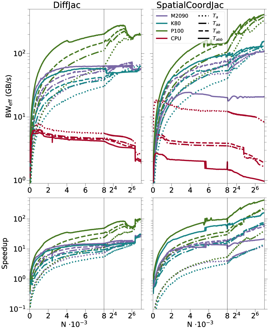
Figure 4: Effective bandwidths (top) and speedups (bottom) for the two Jacobian modules. Line colours and styles respectively indicate different processors and tensor structures. The plots switch from a linear to a logarithmic x-axis scale at a gridsize of 8000.

We now highlight the salient features of Figure 4 and interpret them in light of our theoretical expectation from the computation of $I$ and the pragmatics of our implementation. Our predicted arithmetic intensities $I$ were between $1$ and $5$. Consulting the bottom-left panel of Figure 1, we see that at peak performance $\mathrm{BW}_{\mathrm{eff}}$ should thus be roughly constant in $I$, and thus independent of both the tensor structure and of whether we are performing DiffJac or SpatialCoordJac.

The expected independence of tensor structure and $N_{x}$ can, for the GPUs, be seen in Figure 4. There, the various linestyles representing differing tensor structures appear for each GPU to converge at large $N_{x}$. The exception of the $T_{abb}$ kernel running SpatialCoordJac on the M2090, whose performance can be seen from the top right panel of Figure 4 to be far beneath the other M2090 curves. In this case, the kernel spills registers into local memory. The CPU curves show a much stronger dependence upon tensor structure than predicted when running SpatialCoordJac, and in both cases show a clear negative dependence upon $N_{x}$, presumably since large gridsizes overflow the CPU cache.

For both DiffJac and SpatialCoordJac, the P100 outperforms the M2090 by about a factor of $3$ at large $N_{x}$, as can be seen by comparing the rightmost edges of the $\mathrm{BW}_{\mathrm{eff}}$ lines in Figure 4 for these processors. This is consistent with the expectation from a similar comparison from the bottom left panel of Figure 1. These performances are, however, quantitatively each about a further factor K80 of 3 away from Figure 1’s prediction, indicating that algorithmic redesign could likely further improve performance. This is especially true for the K80, which actually performs slightly less well than the M2090 despite greatly superior specifications. However, as will be shown in Section 4 (specifically Figures 10 and 11), the speedups we have already obtained make Jacobian multiplications a very small part of the overall black hole simulation runtime, so further effort would have little practical impact.

The GPU performance for SpatialCoordJac at large gridsize is, contrary to the expectation from the above analysis (i.e. from the fact that $I$ is quite similar for both operations), consistently about a factor of 2-5 better than for DiffJac, as can be seen by comparing the large $N_{x}$ behaviour of identically styled curves for the GPUs on the left and the right panels of Figure 4. The relevant kernels are coded somewhat differently: all the necessary pointers-to-tensor elements are first collected into a struct, which is passed to the GPU as an argument to the kernel rather than by a CUDA memory copy. All necessary data are then loaded into registers in a way that interleaves memory accesses with computations. This approach may ultimately entail fewer, or better optimized, memory accesses, since no explicit pointer indirections are coded in. The staggered instructions may also improve latency, since less time need be spent waiting for data.

3.4 Spectral Operations: Differentiation and Filtering

$\mathtt{SpEC}$ is named for its use of the pseudospectral collocation method [43, 44, 45, 46, 47]. In this section we describe our porting strategy for two operations, differentiation and filtering, which make explicit use of these methods. Let us begin by introducing spectral methods in the simplest case of $1\mathrm{D}$ PDEs and scalar variables. Spectral methods represent the solution $u(x)$ as a series expansion in basis functions $T_{k}(x)$:

$$u(x)=\sum_{k=0}^{N-1}\tilde{u}_{k}T_{k}(x).$$ (14)

The $\tilde{u}_{k}$ above are called spectral coefficients. The approximation arises because $N$ is finite.

Furthermore, there is a set of collocation points

$$x_{i},i=0,\ldots,N-1.$$ (15)

The function values at the collocation points, $u_{i}\equiv u(x_{i})$, can be computed by a matrix multiplication:

$$u_{i}=\tilde{M}\indices{{}_{i}^{k}}\tilde{u}_{k},$$ (16)

where $\tilde{M}\indices{{}_{i}^{k}}=T_{k}(x_{i})$. For suitable choice of collocation points, the inverse is also a linear transformation:

$$\tilde{u}_{k}=M\indices{{}_{k}^{i}}u_{i}.$$ (17)

We shall refer to Eq. (16) as “SpecToPhys” and to Eq. (17) as “PhysToSpec”.

For a Fourier series and Chebyshev polynomials, the transforms Eq. (16) and Eq. (17) can be evaluated respectively with a fast-Fourier-transform or fast-cosine-transform (we hereafter loosely use the term “FFT” to refer to both possibilities), with $\mathcal{O}(N\log{N})$ complexity scaling rather than the naiively-expected $\mathcal{O}(N^{2})$ for matrix-vector multiplication.

The advantage of spectral methods is that many operations of interest, most notably including differentiation, can also be performed with an FFT, yielding $\mathcal{O}(N\log{N})$ complexity scaling overall. Since, for example, the basis functions form a complete set, their derivatives are linear combinations of basis functions

$$T^{\prime}_{k}(x)=\sum_{k}^{N-1}\tilde{D}\indices{{}_{k}^{l}}T_{l}(x)$$ (18)

which we can exploit to find the differentiation matrix $\tilde{D}\indices{{}_{k}^{l}}$ analytically. Multiplying this matrix by the spectral coefficients $\tilde{u}_{k}$ - which, again for a Fourier series and Chebyshev polyomials, can be done with a $\mathcal{O}(N\log{N})$ FFT - yields $\tilde{u}^{\prime}_{k}$, the spectral coefficients of the solution’s derivative. The real space derivative $u^{\prime}_{i}$ can then be obtained using Eq. (16), with FFT-like scaling overall.

Differentiation accounts for around 20% of $\mathtt{SpEC}$’s total runtime during the SingleBH test (c.f. Figure 3). A second operation called the spectral filter consumes about an additional 30%, and is very similar in form. Here, we perform the same spectral transformations as in (17) and (16), but the matrix in (18) is designed to apply some filtering transformation to the spectral coefficients rather than to compute derivatives. For example, the Heaviside filter zeros out all Fourier modes with a frequency above a certain value.

In practice, $\mathtt{SpEC}$ maintains for each one of these steps a complicated battery of C++ classes that are appropriate for different choices of simulation domain, spectral basis function, and low-level implementation details. Producing hand-written CUDA equivalents of all possible execution pathways would take, to say the least, significant effort. In particular code maintenance would become unmanageable. To avoid this we capitalize on three features of the spectral operations. First, they are all linear maps. Second, a given process will encounter only manageably few unique instances of each. Third, in a practical simulation each unique instance will be encountered by a process very many times.

These properties in concert make feasible a general strategy based on tracing out an explicit matrix representation for each function. Specifically, considering for example the differentiator, we express the entire transformation as an explicit multiplication with a single matrix $D\indices{{}_{j}^{i}}=(\tilde{M}DM)\indices{{}_{j}^{i}}$. We then have

$$u^{\prime}_{j}=D\indices{{}_{j}^{i}}u_{i}$$ (19)

which is mathematically equivalent to the differentiation operation, however the latter is implemented. We can exploit this fact to trace out an explicit matrix representation of $D\indices{{}_{j}^{i}}$. Specifically, we set $u_{i}=\delta_{ik}$ for some $k$, where $\delta_{ik}$ is the Kronecker delta, and then pass this input through the actual extant CPU code. The result is the $k$th column of the matrix $D\indices{{}_{j}^{i}}$. By repeating this procedure for all $k$’s, we trace out the entire matrix in $N_{x}$ function calls.

Having traced out $D\indices{{}_{j}^{i}}$, we maintain an associative array (which we call a dictionary) between it and whatever function input specifies a mathematically-new transform. For the differentiator, this is the gridsize and derivative index, while for the spectral filter, it is the gridsize, the particular filter function to be applied, and in some cases the tensor structure of the input. The extra function calls needed to build the matrix are in practice very few compared to the full number that will be made over the $\mathtt{SpEC}$ runtime, so the extra expense can be ignored.

In general, implementing the spectral operations by explicit matrix multiplications such as Eq. $\eqref{eq:Differentiation}$ will result in worse asymptotic complexity than is achieved by the spectral CPU code, whose expense is dominated by either an FFT or a closely related algorithm. Nevertheless, this approach can be advantageous, especially when viewed as a CPU-to-GPU porting strategy. First, instead of needing to port, optimize, and maintain a parallel GPU code for each of the very many possible spectral transformations, only one or a small number are necessary. Second, the operation counts at low-$N$ can be such that matrix multiplications actually outperform fast transforms at practical gridsizes. Third, FFTs are, in general, much more difficult to parallelize than matrix multiplications, leading to much lower FLOP/s for the former: for example NVIDIA reports large-$N$ double precision operation rates of around 150 GFLOP/s for their cuFFT library running on a K40 GPU [48], compared to near-peak performance in the TFLOP/s regime for matrix multiplication [49] (of course, the FFT involves many fewer operations). Finally, matrix multiplication can be performed by the (cu)BLAS function dgemm, which is possibly the most heavily optimized function in existence.

Let us now consider the realistic case of 3D grids and tensorial solution variables. Usually, the independent tensor components are decoupled, and so generalizing to tensors with $N_{e}$ independent components simply involves a factor of $N_{e}$ extra function calls. But the higher spatial dimensions are qualitatively important, since they change the shapes and characters of the matrix multiplications (or fast transforms).

Let us now consider our port of the differentiator as it works in practice. We start with a function $u(x,y,z)$ available at physical collocation points $u_{ijk}=u(x_{i},x_{j},x_{k})$, and denote by $N_{x}$, $N_{y}$, and $N_{z}$ the physical gridsizes in the subscripted dimension . The full domain topology is an outer product of so-called “irreducible topologies” which cannot be themselves expressed as outer products, and each irreducible topology will be associated with its own set of spectral basis functions. These basis functions will depend on each physical coordinate on their associated domain. For example, on an $\mathcal{I}1\otimes\mathcal{I}1\otimes\mathcal{I}1$ domain, where the irreducible topology $\mathcal{I}1$ is that of a closed line segment, we have three sets of spectral basis functions, and each set depends on only one physical coordinate; we thus call the basis functions 1D. In this case we write

$$u(x,y,z)=\sum_{i,j,k}^{N_{x},N_{y},N_{z}}\tilde{u}_{ijk}T_{i}(x)T_{j}(y)T_{k}(z).$$ (20)

In particular, we can obtain e.g. the $\tilde{u}_{i}$ coefficients, which are all we need to compute the $x$-derivative, without performing the other two sums:

$$\tilde{u}_{\alpha kj}=M\indices{{}_{\alpha}^{i}}u_{ikj}.$$ (21)

The derivatives are again linear combinations of basis functions, we again finish by mapping back to the collocation points, and we again can trace out an explicit matrix representation of the entire operation by feeding delta function input through the CPU code. Denoting this matrix representation by the capital letter corresponding to the physical coordinate upon which it operates, we have

$$u_{abc,d}=\delta_{d1}X\indices{{}_{a}^{i}}u_{ibc}+\delta_{d2}Y\indices{{}_{b}^{j}}u_{ajc}+\delta_{d3}Z\indices{{}_{c}^{k}}u_{abk}.$$ (22)

In some cases SpEC works upon domains composed of irreducible topologies which are not 1D in the above sense - that is, their associated spectral basis functions depend on more than one physical coordinate. The most notable example is spherical shells, with topology $\mathcal{I}1\otimes\mathcal{S}2$. The $\mathcal{I}1$ irreducible topology, representing the radial direction $r$, admits a spectral basis of 1D Chebyshev polynomials that depend only on $r$, but the spherical harmonics $Y_{lm}$ depend on both angular coordinates, $\theta$ and $\phi$. SpEC furthermore in this case uses a compressed, but slightly redundant, spectral representation, so that $\tilde{M}\indices{{}_{i}^{k}}$ is not simply the inverse of $M\indices{{}_{k}^{i}}$. The matrix product $\tilde{M}\indices{{}_{i}^{k}}M\indices{{}_{k}^{j}}$ projects into a subspace of $\{u_{i}\}$.

In this case, we have physical variables $u(r,\theta,\phi)$ available at physical collocation points $u_{klm}=u(r_{k},\theta_{l},\phi_{m})$. The physical gridsizes in the $r$, $\theta$, and $\phi$ directions will be denoted $N_{r}$, $N_{\theta}$, and $N_{\phi}$, while the number of $l$ modes maintained in the spectral representation will be called $N_{l}$ (the number of Chebyshev coefficients is just $N_{r}$). The spectral coefficients are written

$$u(r,\theta,\phi)=\sum_{k=0}^{N_{r}}\sum_{l=0}^{N_{l}}\sum_{m=-l}^{l}\tilde{u}_{klm}\;T_{k}(r)\,Y_{lm}(\theta,\phi),$$ (23)

where $Y_{lm}(\theta,\phi)$ represents the spherical harmonics, and $T_{k}(r)$ a Chebyshev polynomial operating on a suitably rescaled radial coordinate $r$. Because $Y_{lm}(\theta,\phi)$ depend on both the $l$ and $m$ index, computation of either angular derivative requires the entire double sum over both $l$ and $m$. We end up with

$$u_{abc,d}=\delta_{d1}R\indices{{}_{a}^{i}}u_{ibc}+\delta_{d2}\Theta\indices{{}_{bc}^{jk}}u_{ajk}+\delta_{d3}\Phi\indices{{}_{bc}^{jk}}u_{ajk}.$$ (24)

There is now the practical business of expressing these operations as sequences of BLAS calls . $\mathtt{SpEC}$ stores the collocation data $u_{ijk}$ as physically contiguous arrays, so that we are free to join together adjacent indices. We may thus view the data equivalently as a matrix $u_{i,j:k}$ (for the first transform), as a matrix $u_{i:j,k}$ (for the last, or the last two in the $\mathcal{I}1\otimes\mathcal{S}2$ case), or as a set of $k$ submatrices $u_{i,j}$ (for the middle transform), each one of which is multiplied by the appropriate transformation matrix. The colon notation above indicates vectorization into a single index; i.e. $u_{x_{i},y_{j}:z_{k}}$ is a matrix of size $(N_{x},N_{y}N_{z})$.

Since these are just sequences of matrix multiplies, we can easily estimate FLOP and memory transaction counts for each. For $\mathcal{I}1\otimes\mathcal{I}1\otimes\mathcal{I}1$, we first shape the input as an $(N_{x},N_{y}N_{z})$ matrix and multiply with the $(N_{x},N_{x})$ x-transform matrix. Next we shape the input into $N_{z}$ $(N_{x},N_{y})$ submatrices and multiply each with the $(N_{y},N_{y})$ y-transform matrix. Finally, we shape it into an $(N_{x}N_{y},N_{z})$ matrix and multiply that with the $(N_{z},N_{z})$ z-transform matrix. These “reshapings” are just parameter choices to BLAS, and involve actual copies. We repeat this procedure once for each of the $N_{e}$ independent components of the input tensor. The operation count for any particular coordinate $x_{d}$ with size $N_{d}$ has the functional form

$$F=N_{e}N_{x}N_{y}N_{z}(2N_{i}-1).$$ (25)

The x and z transforms involve

$$M=N_{e}(N_{d}^{2}+2N_{x}N_{y}N_{z})$$ (26)

memory operations. As formulated above, however, the y-transform matrix must be read in by the device $N_{z}$ times, with each read acting upon a fraction $1/N_{z}$ of the entire volume data. We thus have

$$M=N_{e}N_{y}N_{z}(N_{y}+2N_{x}).$$ (27)

These memory access estimates somewhat exceed what is strictly required. The transform matrices, for example, are the same for each tensor component, and a kernel could load them from global memory only once for the entire tensor. Optimizing such a kernel to outperform cuBLAS even given the extra accesses would, however, be difficult, especially since matrix multiplication is compute-bound. If $\mathtt{SpEC}$ stored entire tensors as contiguous arrays this could be achieved using the cuBLAS function cublasdgemmStridedBatched. Since this is not in fact the case, we use the above accounting.

In total, we have

$$M =N_{e}(6N_{x}N_{y}N_{z}+N_{x}^{2}+N_{z}N_{y}^{2}+N_{z}^{2})=N_{e}(7N^{3}+2N^{2})$$ (28)

$$F =N_{e}N_{x}N_{y}N_{z}[2(N_{x}+N_{y}+N_{z})-3]=N_{e}(6N^{4}-3N^{3}).$$ (29)

where the rightmost equalities assume $N_{x}=N_{y}=N_{z}\equiv N$, in which case the arithmetic intensity is $I=N\frac{3(2N-1)}{7N+1}\sim\frac{2}{7}N$ (note again that $N$ here is the linear gridsize). Comparing with $I_{\mathrm{eq}}$ from Table 1, we see this operation will be compute-bound at any realistic input size. For $\mathcal{I}1\otimes\mathcal{S}2$, the transform matrix shapes are $(N_{r},N_{r})$ for the radial transform and $(N_{\theta}N_{\phi},N_{\theta}N_{\phi})$ for both of the angular ones. The input reshapings are $(N_{r},N_{\theta}N_{\phi})$ and $(N_{\theta}N_{\phi},N_{r})$. Due to the dependence of the spherical harmonic basis functions on both angular coordinates, the transforms are also over both, even if we only seek e.g. the $N_{\theta}$ derivative. For the same reason, we do not break into $N_{\phi}$ submatrices for the $N_{\theta}$ transform, as we did for $N_{y}$ in $\mathcal{I}1\otimes\mathcal{I}1\otimes\mathcal{I}1$.

Noting that $N_{i}=N_{\theta}N_{\phi}$ for the angular transforms, $F$ and $M$ have the same forms as in (25) and (26). In total, we have

$$M =N_{e}(N_{r}^{2}+2N_{\theta}^{2}N_{\phi}^{2}+6N_{r}N_{\theta}N_{\phi})$$ (30)

$$F =N_{e}N_{r}N_{\theta}N_{\phi}[2N_{r}+4N_{\theta}N_{\phi}-3].$$ (31)

In practical simulations, the resolutions $N_{r}$, $N_{\theta}$, and $N_{\phi}$ can differ widely from one another. For our benchmarks we therefore distribute points by two prescriptions. The “SingleBH” benchmarks are on spherical shells that mirror those found in $\mathtt{SpEC}$’s isolated black hole evolutions. Resolution is controlled by a resolution parameter $k=0,1,\ldots,10$, in terms of which we have $N_{r}=9+4k$, $N_{\theta}=6+2k$, $N_{\phi}=4k+12$, and thus $N_{\theta}N_{\phi}=8k^{2}+48k+72$. The “BBH” benchmarks use roughly the same point distribution as used initially for the spherical shells closest to the apparent horizons of black hole binaries in an actual BBH simulation . The radial resolution is comparatively much lower in this case. Specifically we have $N_{r}=4+k$, $N_{\theta}=7+2k$, $N_{\phi}=4k+14$, $k=1,2,\ldots,16$, and thus $N_{\theta}N_{\phi}=8k^{2}+56k+98$. For SingleBH, we have

$$M =N_{e}(128k^{4}+1728k^{3}+8512k^{2}+18216k+14337)\sim 128N_{e}k^{4}$$ (32)

$$F =N_{e}(1024k^{5}+14848k^{4}+85536k^{3}+244728k^{2}+347760k+196344)\sim 1024N_{e}k^{5}.$$ (33)

The arithmetic intensity $I=13.7$ for $k=0$ and grows approximately linearly thereafter. For the BBH benchmarks we have

$$M =N_{e}(128k^{4}+1840k^{3}+9937k^{2}+23892k+21576)\sim 128N_{e}k^{4}$$ (34)

$$F =N_{e}(256k^{5}+4624k^{4}+33368k^{3}+120252k^{2}+216426k+155624)\sim 256N_{e}k^{5}.$$ (35)

This arithmetic intensity $I$ starts at $7.2$. The operations will clearly be compute-bound in all cases. Of course, equal $k$ implies different total gridsize between cases, so it is difficult to estimate performance at equal gridsize from the above. To do that we refer to Figure 5, where $M$, $F$, and $I$ are shown for each of the three grids. With $I$ in hand as a function of gridsize, we can refer once more to Figure 1 to predict ideal effective processing rates $P_{\mathrm{eff},\mathrm{opt}}$ from Eq. (6), which we plot against gridsize in the bottom panels of Figure 5.

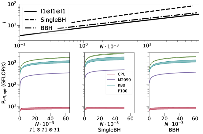
Figure 5: Top: Arithmetic intensity $I$ plotted as a function of gridsize $N$ for the matrix multiply differentiator operating on $\mathcal{I}1\otimes\mathcal{I}1\otimes\mathcal{I}1$, and upon $\mathcal{I}1\otimes\mathcal{S}2$ with the SingleBH and BBH gridpoint distributions. For $\mathcal{I}1\otimes\mathcal{I}1\otimes\mathcal{I}1$ these estimates also apply to the spectral filter. Bottom: theoretical zero-latency processing rate $P_{\mathrm{eff,opt}}$ for each of the benchmarked devices as a function of gridsize. Note that the CPU uses a more efficient (at large gridsize) algorithm, so these lines do not bound its performance.

We now turn our attention to spectral filtering, and return focus initially to $\mathcal{I}1\otimes\mathcal{I}1\otimes\mathcal{I}1$ topologies. Spectral filtering of 1D basis functions is similar to differentiation, the only difference being the specific form of the transformation matrix. In Figure 6 we thus show the performance of both the differentiator and the spectral filter operating on an $\mathcal{I}1\otimes\mathcal{I}1\otimes\mathcal{I}1$ topology. Comparing the performance of the spectral filter with that of the differentiator, we see near-identical behaviour on the CPU. On the GPU we get qualitatively similar but somewhat worse performance from the spectral filter. This is due to the extra cost in the latter case of looking up the cached transform matrices. Since the differentiator always implements the same transformation, we can store the relevant matrices as private members of a differentiator C++ class. For the spectral filter, there are very many possible transformations, which necessitates a more complicated caching strategy. While the performance difference is likely unimportant in practice, the lookup could probably be substantially optimized if necessary.

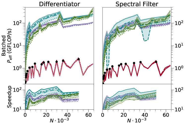
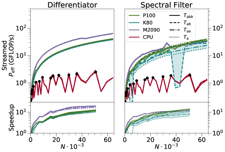
Figure 6: Effective processing power $P_{\mathrm{eff}}$ and speedups vs. one CPU core for the matrix multiply differentiator (left) and spectral filter (right) acting on an $\mathcal{I}1\otimes\mathcal{I}1\otimes\mathcal{I}1$ topology. Input tensor structures differ by linestyle, while the devices of Table 1 differ by colour. The CPU algorithm exhibits sharply gridsize-dependent performance, and we compute speedups only at peaks, marked with black circles. In the top (bottom) panels, we use the batched (streamed) API, which in this case performs better (worse).

The CPU curves in Figure 6 are computed using the same operation count model as we use in the GPU case, which is $O(N^{4})$ in the linear gridsize $N$. However, the CPU in practice uses an FFT on the transformed basis function, and so its true scaling is, for favourable collocation point choices, $O(N^{3}\log{N})$. Because our model underestimates the true CPU FLOP count the CPU performance curves on Figure 6 can in principle exceed the CPU’s theoretical performance (c.f. Figure 5), although in this case they do not. The scaling coefficients at lower gridsizes are better for matrix multiply, which is why the latter alogorithm can be favourable, especially given superior hardware. Unfavourable collocation point choices can furthermore affect the true CPU FLOP count by about an order of magnitude, causing the jagged behaviour of the CPU curves in Figure 6. When computing the speedup, we use only the “peak” points (chosen by eye), and have plotted a linear interpolation between these.

The performance of the CPU algorithm is roughly independent of the number of independent tensor components $N_{e}$. For the GPU algorithm we can get some dependence upon the latter. The individual matrix multiplication sizes are on the order of the linear gridsize, between around $10$ and $40$. Neither cuBLAS nor the GPU itself are very well optimized for such small matrix multiplications, which cannot individually utilize all the streaming multiprocessors of the device. This likely accounts for the underperformance of the GPUs compared to their theoretical processing powers. The reason for the performance dip on the K80 $T_{ab}$ curves around $N=40000$ is unclear.

We thus use one of two concurrency strategies that allow multiple small kernels to exhibit some parallelism. The first strategy, called “streamed”, attempts to run the kernels concurrently using CUDA streams. These are a CUDA API feature that allow kernels to be run asynchronously with the CPU and with one another. This approach cannot achieve concurrent execution for very small kernels for which the kernel launch overhead of about 20 $\mu$s is an important expense, since only one kernel can be prepared for launch at one time. Also, since the individual kernels have no knowledge of one another, $\mathtt{cuBLAS}$ must tune them as if they were to run synchronously, which may result in suboptimal tuning overall.

The second strategy, called “batched”, runs each separate matrix transformation as a single call to the API function $\mathtt{cublasDgemmBatched}$. This function performs an identical matrix multiplication on a series of matrices, given to the API as an array of pointers. Using it incurs some extra overhead, since this array must be first copied to the GPU . The batched API can in many cases give superior performance to streamed multiplications. Generically, it will be the better choice for numerous multiplications on small kernels. In that case the batched API can save on launch overhead, and may also make superior tuning choices since it is aware of the full operation.

Sometimes, however, the streamed strategy is favourable. It is not easy to predict which will be which except by experiment. We have, for example, performed benchmarks which show that for some matrix shapes the batched strategy is a factor of 2-5 faster even when only a single (small) matrix is being operated upon. In other cases, we have found that the batched API is modestly superior on some cards, but that streamed calls are almost an order of magnitude better on newer ones, presumably because of new GPU features being exploited on newer cards. Because of this, we have experimented with both strategies in all our benchmarks.

On $\mathcal{I}1\otimes\mathcal{I}1\otimes\mathcal{I}1$, the batched strategy consistently gives an improvement of about an order of magnitude, with larger tensors giving a greater advantage. This topology involves very many individually tiny matrix multiplications ($N_{e}(2+N)$ in total), so this is perhaps to be expected. Especially when using the batched strategy, we get very impressive speedups overall, of between 10 and 100X. This is despite the observed performance being about an order of magnitude beneath our theoretical prediction. It must be stressed that our CPU benchmarks use only 1 CPU core, which has a fairly modest clock frequency of 2.0 GHz. While realistic for $\mathtt{SpEC}$ this would in most circumstances be a very unusual comparison. 6 CPU cores running at 3-4GHz might be more typical of modern hardware, which would give about an order of magnitude speedup assuming linear scaling with parallelism (which $\mathtt{SpEC}$ cannot achieve).

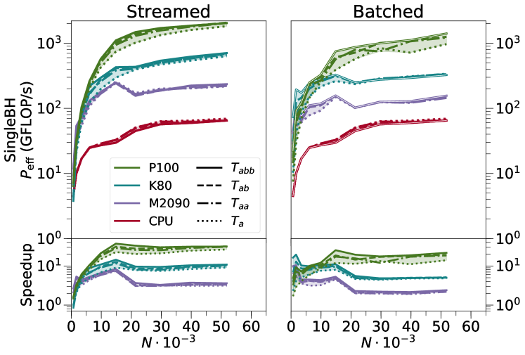
Figure 7: Effective processing power $P_{\mathrm{eff}}$ and speedups vs. one CPU core for the matrix multiply differentiator acting on a $\mathcal{I}1\otimes\mathcal{S}2$ topology using the ‘SingleBH’ gridpoint distribution, using the streamed (left) and batched (right) concurrency strategy. In terms of the resolution parameter $k$, ‘SingleBH’ has $N_{r}=9+4k$, $N_{\theta}=6+2k$, and $N_{\phi}=2N_{\theta}$. Different linestyles indicate differing tensor structures as indicated in the legend, with a colour fill between $T_{abb}$ and $T_{a}$ (performance of the intermediate structures is usually, but not always, bounded by these).

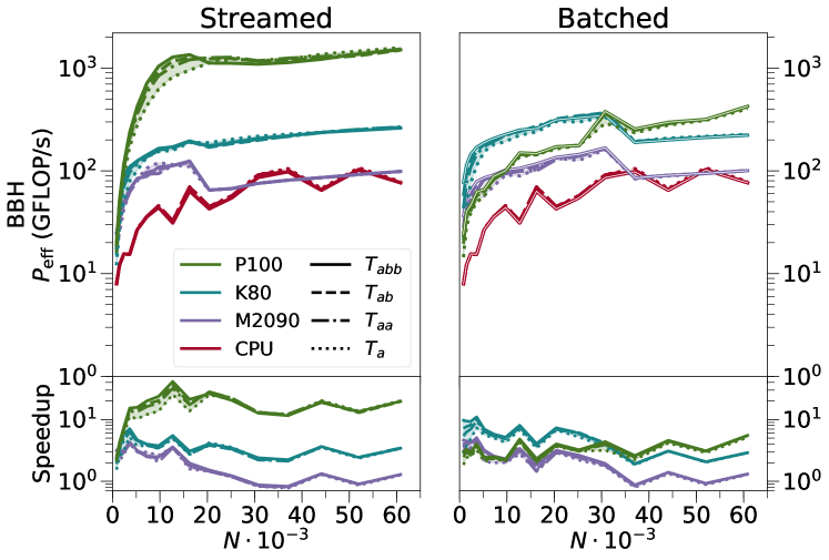
Figure 8: Effective processing power $P_{\mathrm{eff}}$ and speedups vs. one CPU core for the matrix multiply differentiator acting on a $\mathcal{I}1\otimes\mathcal{S}2$ topology using the ‘BBH’ gridpoint distribution, using the streamed (left) and batched (right) concurrency strategy. In terms of the resolution parameter $k$, ‘BBH’ has $N_{r}=4+k$, $N_{\theta}=7+2k$, and $N_{\phi}=2N_{\theta}$. Formatting and axis scales are identical to those in Figure 7.

We now turn to the results on spherical shells $\mathcal{I}1\otimes\mathcal{S}2$, where a more complex picture will emerge than for $\mathcal{I}1\otimes\mathcal{I}1\otimes\mathcal{I}1$. We first discuss the differentiator, results from which are summarized in Figures 7-8. Especially for larger gridsizes and especially on the P100 our GPU performance is quite comparable to the predicted peak performance shown in the lower panels of Figure 5. The CPU performance, on the other hand, exceeds both this prediction, and the CPU’s theoretical processing power. The expense of the transform is dominated by the angular sector in both cases. On the CPU, the $\phi$ transform is done with an FFT, and the $\theta$ by a matrix multiply, yielding $N_{r}(N_{\theta}N_{\phi})^{3}\log{(N_{\theta}N_{\phi})}$ scaling, compared to the $N_{r}(N_{\theta}N_{\phi})^{4}$ scaling of our model. This gives a ratio $N_{\theta}N_{\phi}/\log{(N_{\theta}N_{\phi})}$, which is a larger factor than for $\mathcal{I}1\otimes\mathcal{I}1\otimes\mathcal{I}1$, since $N_{\theta}N_{\phi}$ is larger. This is particularly true for the BBH case, explaining the improved CPU performance of BBH vs. SingleBH.

For the SingleBH grid we achieve an appreciable speedup of between $5$ and $30$X throughout. Performance is consistently better for the streamed strategy in this case, perhaps because the individual angular multiplications are now large enough that $\mathtt{cuBLAS}$ can make effective tuning choices. For BBH, where the spectral algorithm gives the largest advantage, the GPU advantage is more modest and the CPU actually exceeds the M2090 performance in some cases. This is unfortunately the more realistic gridsize choice for production simulations.

The batched vs. streamed picture is here much less clear than it was for $\mathcal{I}1\otimes\mathcal{I}1\otimes\mathcal{I}1$. On the P100 the streamed strategy is greatly advantageous, whereas batched is modestly superior on the other cards. GPU performance seems in most cases to scale up to some kind of threshold, after which point there is a sharp dip and a new slow scaling upwards (for example at around gridsize 30000 for the BBH batched K80 and M090 runs, or 15000 on SingleBH). This may be due to $\mathtt{cuBLAS}$ switching here to a new kernel optimized for multiplications with a large shared dimension. In that case, kernels need to read much more data than they will end up writing to global memory, which limits parallelism.

We now turn to spectral filtering on $\mathcal{I}1\otimes\mathcal{S}2$ shells. The radial filter, along $\mathcal{I}1$, is handled in the same way as the $x$-dimension in $\mathcal{I}1\otimes\mathcal{I}1\otimes\mathcal{I}1$. In our benchmarks, as in production runs, we do not include a filter along the $r$-axis.

For spectral filtering of 2D basis functions, the filtering transformation will normally couple together elements from different components of a tensor. This necessitates a different approach, especially since the relevant coupling will be very sparse. For filtering on $\mathcal{I}1\otimes\mathcal{S}2$ we therefore break the operation into three steps. During “PhysToSpec” (“SpecToPhys”), each of the input tensor $U_{ijk...}$’s $N_{e}$ independent components are separately transformed as in Eqs. (17) and (16). In physical space, each tensor component is viewed as a $(N_{r},(N_{\theta}N_{\phi}))$ matrix, and the spectral transform matrix has dimensions $((N_{\theta}N_{\phi}),N_{s})$, where the spectral dimension $N_{s}$ (very roughly $N_{\theta}N_{\phi}/2$) is the number of coefficients of the spectral representation. Thus,

$$F =N_{e}N_{r}N_{s}(2N_{\theta}N_{\phi}-1),$$ (36)

$$M =N_{e}(N_{r}N_{\theta}N_{\phi}+N_{r}N_{s}+N_{\theta}N_{\phi}N_{s}).$$ (37)

The “SpecToPhys” transformation simply swaps $N_{\theta}N_{\phi}$ with $N_{s}$ in the above.

We choose BLAS parameters such that the PhysToSpec transform maps the different tensor components into a single contiguous $N_{r}N_{e}N_{s}$ array, which we view as an $(N_{e}N_{s},N_{r})$ matrix. The filter is then implemented by multiplying with an $(N_{e}N_{s},N_{e}N_{s})$ transform matrix which couples the $N_{e}$ distinct tensor components. Typically, only about 10% or fewer of the entries in this matrix are nonzero, and so it becomes worthwhile to store it in a sparse format. We use the CSR format [50] because it is fairly simple and well-supported by the NVIDIA sparse algebra package $\mathtt{cuSPARSE}$.

The complexity of the filtering step depends somewhat sensitively upon the actual structure of the sparse filtering matrix and upon the details of the matrix multiplication algorithm. The sparsity of the filtering matrix will in turn depend on what filter is being applied, so we profile using two different such functions, which we call Heaviside (a Heaviside filter) and ExpCheb (an exponential Chebyshev function). We use the $\mathtt{cuSPARSE}$ algorithm $\mathtt{dcsrmm2}$. The cuSPARSE documentation [50] describes this algorithm as memory bound, with an approximate complexity of $N_{e}N_{s}[sN_{e}N_{s}(N_{e}N_{s}+1)+2N_{r}]$. Here the sparsity factor $s=Nnz/(N_{e}^{2}N_{s}^{2})$, while $Nnz$ is the number of nonzero entries in the sparse matrix.

The benchmarks in this case are illustrated by Figure 9. GPU performance is dominated by the (dense) spectral transform multiplications, and so the results are comparable to, but worse than, those of the differentiator acting on $\mathcal{I}1\otimes\mathcal{S}2$, shown in Figures 7-8. The worse performance is due to the larger number of operations, the extra time needed for matrix lookup, and the more asymmetrical matrix dimensions. Speedups, however, are in many cases higher for the spectral filter, because in that case the CPU performance is much more sensitive to the number of independent components of the input tensor. Curiously, the CPU processes $T_{ab}$ considerably more efficiently than $T_{aa}$, even though the latter has fewer components. As for the differentiator, the streamed concurrency strategy gives somewhat better results overall for SingleBH. For BBH, the batched API is marginally superior except on the P100, where the streamed strategy outperforms by about a factor of 2 (c.f. the hollow lines in the lower panels of Figures 10 and 11).

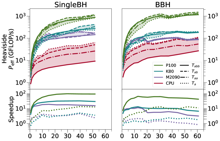
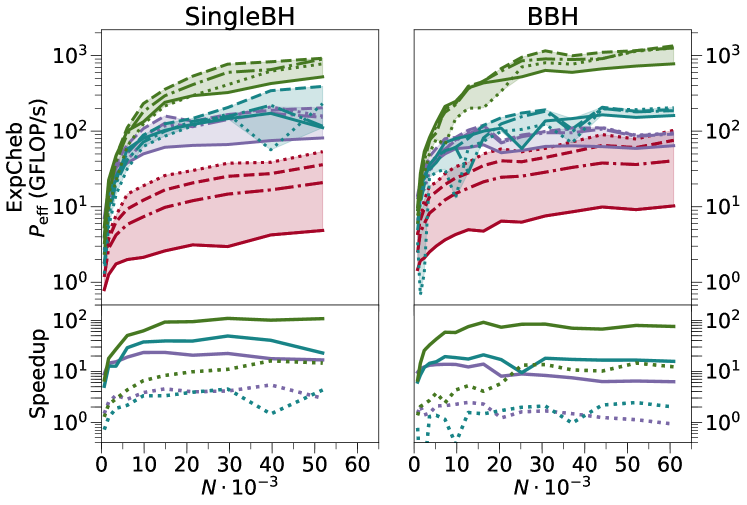
Figure 9: Effective processing power $P_{\mathrm{eff}}$ and speedups vs. one CPU core for the matrix multiply spectral filter acting on an $\mathcal{I}1\otimes\mathcal{S}2$ topology for ‘SingleBH’ (left) and ‘BBH’ (right) gridpoint distributions. We study two filter functions, Heaviside (top) and ExpCheb (bottom). Speedups are shown only for $T_{\mathrm{abb}}$ and $T_{\mathrm{a}}$. Line colours (and fill) distinguish between processors, and line styles between tensor structures. Here we only profile the streamed API, which generally performs better.

3.5 $\mathtt{DataMesh}$ Operations, Apply BCs, GHEqns

Apart from the individually-significant operations described above, $\mathtt{SpEC}$ contains numerous operations on our array class, $\mathtt{DataMesh}$, which are distributed too widely throughout the code to port individually. To deal with these we use our automatic porting system, TLoops. While TLoops is a separate subject in itself, we briefly describe it here to keep this paper self-contained.

TLoops furnishes a set of C++ classes to represent arrays, tensors, indices over tensors, and operations between tensors. These classes are based on templates, which recursively iterate at compile time to form unique types for each tensor manipulation written in the $\mathtt{SpEC}$ code. After compilation a separate executable can be used to generate valid CUDA code for each unique operation. This can then be linked back to a separate checkout of $\mathtt{SpEC}$. In this way all manipulations of $\mathtt{DataMesh}$ throughout the code can be ported at once.

If no changes are made to the code at all, $\mathtt{DataMesh}$ operations ported automatically with TLoops will typically show only a modest speedup or even a slowdown at lower gridsizes, due to large amounts of launch overhead incurred by loops over kernel launches. Even in the case of a small slowdown, however, the automatic porting yields a net benefit since it avoids numerous CPU-GPU synchronizations that would otherwise occur around the explicitly ported modules.

Much of the slowdown comes from the operations collected as ApplyBCs. These functions operate mostly on angular slices at the boundaries of the domains, which have about an order of magnitude fewer points than do the full three-dimensional volume arrays: a shell with $(N_{r},N_{\theta},N_{\phi})$ gridpoints has boundaries with only $(N_{\theta},N_{\phi})$ gridpoints, and $N_{r}$ is typically around $10$. Such operations can be a considerable bottleneck for two reasons. First, the code that extracts and inserts these two-dimensional slices out of and into the volume involves an unavoidably strided data access that is very inefficient to port on the GPU. It is nevertheless best to do so in order to avoid extra synchronizations. Second, the ApplyBCs operations are simply very small and very numerous. Launch overhead impairs their performance severely.

We deal with this by leaving boundary data on the CPU throughout. TLoops expressions check the dimension of the relevant $\mathtt{DataMesh}$es, and execute on the GPU only for dimension 3 or higher. The $\mathtt{DataMesh}$ copy constructor also transfers data on the host (rather than the device) for dimension 1 or 2, unless the data is on the device already (for dimension 3 we always synchronize with the GPU and copy there). TLoops still somewhat impairs the performance of the ApplyBCs operations since the boundary arrays must be copied to the GPU whenever they are to be extracted from or inserted to the volume. But the net effect is a speedup.

Launch overhead can be mitigated even further by operating on whole tensors with a single kernel. Code must be modified to do this, so it is not practical to do throughout, but it does provide a very simple and convenient porting strategy for complicated operations. We have used this strategy to port the GHEqns, which solve the Einstein equations. This allows for about a 10X speedup at realistic gridsize without writing any explicit CUDA code (c.f. Section 4.4).

4 Benchmarks of Overall Code

Figures 10 and 11, finally, summarize our entire GPU porting results. These figures show benchmarks from runs of $\mathtt{SpEC}$ upon isolated black hole test cases. Shown are two gridsizes, SingleBH and BBH, identical to the eponymous gridsizes used in the performance analysis of the differentiation and the spectral filter in 3.4. Compared to the SingleBH tests, the BBH tests have a relatively larger angular resolution at constant gridsize. We ran each benchmark five times for 110 timesteps, and collected results between timesteps 5 and 105. As in the previous benchmarks, the plotted results are the median times over the five runs.

These single black hole runs evolve a stationary, single black hole with a spin of $0.5$ using the generalized harmonic equations. Surrounding the black hole are two $\mathcal{I}1\otimes\mathcal{S}2$ subdomains with identical resolutions. Apart from being numerically simpler, the isolated case differs from a full binary black hole simulation in several ways. A binary black hole simulation would have a much more diverse set of domains, and would involve AMR, which we have not considered here. Binary evolutions also involve interpolations and computations on the apparent horizons of the black holes, which can be importantly expensive. Finally, binary evolutions use MPI, which assigns each individual domain to a different CPU core. In our full port, each would instead be assigned to a separate GPU. However, in these tests, we do our computations on the two respective spheres in serial.

The GPU performance is especially strong in the (less realistic) SingleBH gridpoint distribution, which has more points in the radial direction at a given gridsize. Generally we see comparable performance for both distributions as expected from our individual benchmarks in the per-module speedups, although the differentiator on the BBH distribution performs somewhat worse than expected. The GHEqns, which are ported automatically using TLoops, show particularly strong performance - a 100X speedup on the P100 - especially given that no algorithmic redesign was required here.

The differentiator, and to a lesser extent the filter, remains important to the overall wallclock time, particularly for P100. Indeed, the overall speedup is limited by this module, especially on the M2090. Porting the spectral algorithm explicitly on spheres may be worthwhile.

Much of the speedup is limited by the ApplyBCs and the Other operations. The latter are mostly a large mass of tensor manipulations which have not been explicitly replaced with TLoops expressions. We expect a further speedup of these modules by 2-15X could be achieved by doing so, due to both savings in launch overhead and extra parallelism over tensor structure.

The ApplyBCs operations present a more serious challenge. These operations are on arrays of dimension 2, which we have purposely left on the CPU throughout. The performance of these operations is thus limited in principle by the CPU performance. It will usually be somewhat worse than this, because these low-dimension arrays arise as slices of higher-dimensional data living on the CPU, and extracting these slices requires a GPU-CPU memory transfer. The arrays in question are so small that kernel launch overhead is the dominant expense if they are kept on the GPU throughout, to a sufficient extent that the memory copies are still cheaper overall. However, porting to TLoops may mitigate this.

Parallelization of a particular domain across multiple GPUs would not be worthwhile, as our essential problems throughout have been code complexity and the small size of our operations compared to those for which the GPU is optimized. However, multiple GPUs can still be leveraged by assigning one domain to each, which should give roughly linear scaling.

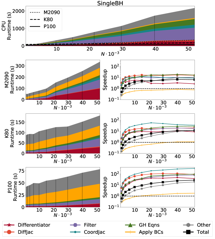
Figure 10: $\mathtt{SpEC}$’s overall performance broken down by module using the SingleBH gridpoint distribution. On the top and left, we show “stack” plots for each benchmarked device. The height of each slice is the runtime of its module, and the total height is the overall runtime. Dotted vertical lines mark the profiled resolutions. On the CPU stack (top), we overlay the GPU runtimes as black lines. The grey stack (‘Other’) represents all modules not otherwise included. On the right, we show the speedup of each module, with identical colouring as on the left, and the total speedup in black.

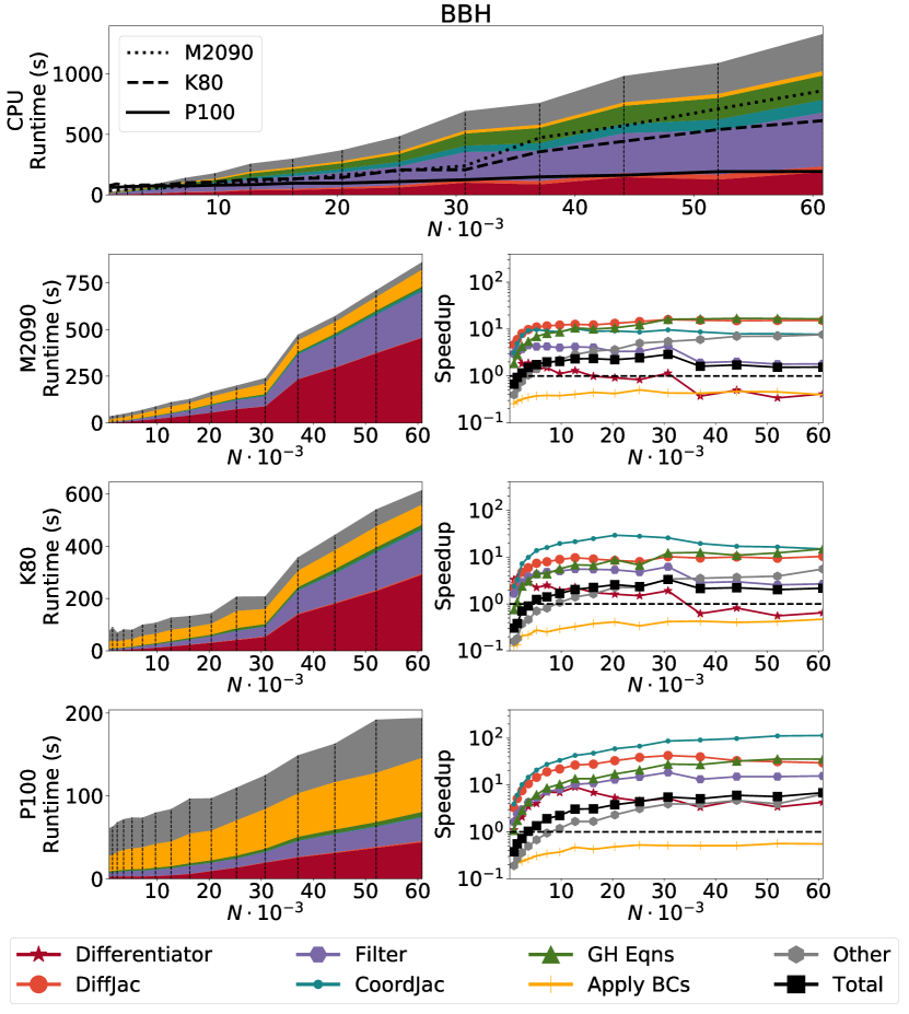
Figure 11: $\mathtt{SpEC}$’s overall performance broken down by module using the BBH gridpoint distribution. The plots are formatted in the same way as Figure 10.

5 Conclusions

We have performed a CPU to GPU port of the portions of the numerical relativity code $\mathtt{SpEC}$ relevant to single black hole simulations. Our combined strategy of explicit porting for the Jacobian multiplications, semi-automatic porting for spectral operations that can be written as matrix transformations, and completely automatic porting for the many scattered tensor operations throughout the code gives comparable to peak performance for many of these modules, module-to-module speedups compared to one CPU core ranging from 10 to 100X, and overall speedups of between 2-10X. Due to its reliance on prepackaged libraries, our port also generally shows improved performance when run on newer hardware without requiring extra tuning.

The next step in GPU-porting will be to completely port the code so that the accelerated version can be used for binary black hole simulations. Binary black hole runs differ from the single black hole case in three main ways. First, they involve a larger and more diverse set of computational domains than the two spherical shells considered in the single black hole case. Second, those domains must communicate in parallel using MPI. Third, production runs involve apparent–horizon finding. Let us comment on each of these issues in turn:

The specific individual domains involved in a binary black hole run are spherical shells ($\mathcal{I}1\otimes\mathcal{S}2$), cubes ($\mathcal{I}1\otimes\mathcal{I}1\otimes\mathcal{I}1$), and cylindrical shells ($\mathcal{I}1\otimes\mathcal{B}2$). Since our port relies on “black box” linear transformations, the most important feature of these domains from our perspective is their spectral dimension; i.e. $\mathcal{S}2$ (dimension 2) vs $\mathcal{I}1$ (dimension 1). As documented in Section 3 our port performs best relative to the CPU spectral algorithms in the dimension 1 case. Our single black hole runs, however, were profiled on dimension 2 spherical shells, which apart from being dimension 2 make use (on the CPU) of heavily-optimized FORTRAN modules for the efficient manipulation of spherical harmonics. Internal to each domain, we can therefore expect performance during production runs at least equal to, and probably better than, during the single black hole simulations considered in the present work.

Moving from one subdomain to many will change the relative importance of boundary condition operations (‘ApplyBCs’) compared to volume data processing. Since the ApplyBCs modules were problematic for our port, this could conceivably impair scaling to larger domains. However, we in fact expect this scaling to be favourable. SpEC runs use ApplyBC in three distinct cases: (i) at ‘internal’ boundaries between neighboring domains, the characteristic variables are computed and used as boundary conditions on the neighboring subdomain; (ii) at the external outermost boundary, rather complex constraint-preserving boundary conditions are applied [51]; and (iii) at BH excision boundaries, no boundary conditions are applied at all. The SingleBH test-case presented here uses two domains, leading to two internal boundaries and one external boundary with the constraint preserving boundary conditions (plus one ‘no-op’ at the inner excision boundary).

For a full binary black hole simulation, there will still be only one outer boundary where the expensive (ii) boundary condition is applied. The number of inner boundaries (i) will grow in proportion to the number of domains (plus there will be two ‘no-op’ black hole excision boundaries). Therefore, we expect that the computational cost of ApplyBC relative to the volume operations will decrease as more domains are added, because of the smaller fraction of boundaries with the expensive (ii) boundary conditions.

There is also the practical matter of interfacing MPI with a multi-GPU code. In our case this is quite simple since our model of parallelism has each GPU operating on data-independent domains. The business of ‘load-balancing’ between independent processors is already handled by mature SpEC code.

The effect of apparent horizon processing on performance is harder to predict. The apparent horizon will normally not be confined to a particular simulation domain. Finding it thus requires data from multiple domains, and thus entails addition CPU-GPU communication steps. After finding the horizon, data must be interpolated upon it, an operation which can be cast as another linear transformation. Without further study, it is difficult to speculate on the overall impact this will have.

A recurring question in GPU computing is whether the quite substantial effort of a GPU-port is worthwhile at the end. Reorganizing the structure of filtering and derivative-computation toward fewer, larger BLAS calls was a requirement for the CUDA port presented here. This same reorganization also had the side-benefit of speeding up the CPU version of these modules by a factor of $\sim\!\!2$, and has thus benefited SpEC in general. An alternative approach to GPU porting would be to implement efficient multi-threaded processing across CPU-cores, using e.g. OpenMP. The idea is to spread each domain over multiple compute-cores, possibly across an entire compute node, and so enable a different layer of parallelism. This would still entail separate coding efforts for each major part of the code which we had to deal with in the present work, among them filtering, derivatives, general computations. Past efforts within the SXS collaboration to utilize OpenMP to speed up tensor-computations like GHEqns have not led to a speed-up. Especially given the new opportunities afforded by the automatic code generation in TLoops, it would be worthwhile to renew such efforts.

6 Acknowledgments

We thank Nils Deppe and Mark Scheel for helpful discussions. Calculations were performed with the SpEC-code [32]. We gratefully acknowledge support from NSERC of Canada, form the Canada Research Chairs Program, and from the Canadian Institute for Advanced Research. Some calculations were performed at the SciNet HPC Consortium [52]. SciNet is funded by: the Canada Foundation for Innovation (CF) under the auspices of Compute Canada; the Government of Ontario; Ontario Research Fund (ORF) – Research Excellence; and the University of Toronto.

References

References

- [1] Pretorius F 2005 Phys. Rev. Lett. 95 121101
- [2] Pretorius F 2005 Class. Quant. Grav 22 425
- [3] Campanelli M, Lousto C O, Marronetti P and Zlochower Y 2006 Physical Review Letters 96 111101
- [4] Baker J G, Centrella J, Choi D I, Koppitz M and van Meter J 2006 Phys. Rev. Lett. 96 111102 (Preprint gr-qc/0511103)
- [5] Campanelli M, Lousto C O and Zlochower Y 2006 Phys. Rev. D 73(6) 061501 URL https://link.aps.org/doi/10.1103/PhysRevD.73.061501
- [6] Mroue A H et al. 2013 Phys. Rev. Lett. 111 241104 (Preprint 1304.6077)
- [7] Chu T, Fong H, Kumar P, Pfeiffer H P, Boyle M, Hemberger D A, Kidder L E, Scheel M A and Szilagyi B 2016 Class. Quant. Grav. 33 165001 (Preprint 1512.06800)
- [8] Bohé A, Shao L, Taracchini A, Buonanno A, Babak S, Harry I W, Hinder I, Ossokine S, Pürrer M, Raymond V, Chu T, Fong H, Kumar P, Pfeiffer H P, Boyle M, Hemberger D A, Kidder L E, Lovelace G, Scheel M A and Szilágyi B 2017 Phys. Rev. D 95(4) 044028 URL https://link.aps.org/doi/10.1103/PhysRevD.95.044028
- [9] Pan Y, Buonanno A, Taracchini A, Kidder L E, Mroue A H et al. 2013 Phys. Rev. D 89 084006 (Preprint 1307.6232)
- [10] Taracchini A, Buonanno A, Pan Y, Hinderer T, Boyle M, Hemberger D A, Kidder L E, Lovelace G, Mroue A H, Pfeiffer H P, Scheel M A, Szilagyi B, Taylor N W and Zenginoglu A 2014 Phys. Rev. D 89 (R) 061502 (Preprint 1311.2544)
- [11] Abbott B P et al. (LIGO Scientific Collaboration, Virgo Collaboration) 2016 Phys. Rev. Lett. 116(6) 061102 (Preprint 1602.03837) URL http://link.aps.org/doi/10.1103/PhysRevLett.116.061102
- [12] Abbott B P et al. (LIGO Scientific Collaboration, Virgo Collaboration) 2016 Phys. Rev. D 93(12) 122003 submitted to to PRD (Preprint 1602.03839)
- [13] Abbott B P et al. (Virgo, LIGO Scientific) 2016 Phys. Rev. D94 064035 (Preprint 1606.01262)
- [14] Abbott B P et al. (Virgo, LIGO Scientific) 2017 Class. Quantum Grav. 33 104002 (Preprint 1611.07531)
- [15] Lovelace G et al. 2016 Class. Quant. Grav. 33 244002 (Preprint 1607.05377)
- [16] Cadonati L et al. (LIGO Scientific Collaboration, Virgo Collaboration) 2015 The LSC-Virgo white paper on gravitational wave searches and astrophysics URL https://dcc.ligo.org/LIGO-T1500055/public
- [17] Lewis A G M, Zimmerman A and Pfeiffer H P 2017 Classical and Quantum Gravity 34 124001 URL http://stacks.iop.org/0264-9381/34/i=12/a=124001
- [18] Zink B 2008 CCT Technical Report Series, CCT-TR-2008-1
- [19] Zink B 2011 Horizon: Accelerated general relativistic magnetohydrodynamics 1102.5202
- [20] Yang Q, Du Z, Cao Z, Tao J and Bader D A 2016 Scientific Programming
- [21] Cao Z, Yo H J and Yu J P 2008 Phys. Rev. D 78(12) 124011 URL https://link.aps.org/doi/10.1103/PhysRevD.78.124011
- [22] Galaviz P, Brügmann B and Cao Z 2010 Phys. Rev. D 82(2) 024005 URL https://link.aps.org/doi/10.1103/PhysRevD.82.024005
- [23] Chen F 2015 J. Sci. Comput. 62 575–600 ISSN 0885-7474 URL http://dx.doi.org/10.1007/s10915-014-9868-3
- [24] Teukolsky S A 1973 apj 185 635–648
- [25] Khanna G 2010 Int. J. Model. Simul. Sci. Comput. 1 147 (Preprint 0911.1565)
- [26] Choudhary N, Ginjupalli R, Navada S and Khanna G 2010 Arxiv preprint arXiv:1010.3816
- [27] Khanna G and McKennon J 2010 Comput. Phys. Commun. 181 1605–1611 (Preprint 1001.3631)
- [28] Khanna G 2013 J. Sci. Comput. 56 366–380 ISSN 0885-7474 URL http://dx.doi.org/10.1007/s10915-012-9679-3
- [29] Herrmann F, Silberholz J and Tiglio M 2011 Black hole simulations with cuda GPU Computing Gems: Emerald Edition (Morgan Kaufmann Publishers) URL http://www2.cscamm.umd.edu/publications/gpugems_CS-11-13.pdf
- [30] Brügmann B 2013 Journal of Computational Physics 235 216 – 240 ISSN 0021-9991 URL http://www.sciencedirect.com/science/article/pii/S0021999112006833
- [31] Blazewicz M, Hinder I, Koppelman D M, Brandt S R, Ciznicki M, Kierzynka M, L offler F, Schnetter E and Tao J 2013 Scientific Programming 21 130360
- [32] http://www.black-holes.org/SpEC.html
- [33] Press W H, Teukolsky S A, Vetterling W T and Flannery B P 2007 Numerical Recipes 3rd Edition: The Art of Scientific Computing 3rd ed (New York, NY, USA: Cambridge University Press) ISBN 0521880688, 9780521880688
- [34] Scheel M A, Pfeiffer H P, Lindblom L, Kidder L E, Rinne O and Teukolsky S A 2006 Physical Review D 74 104006
- [35] Kirk D B and Hwu W m W 2010 Programming Massively Parallel Processors: A Hands-on Approach (30 Corporate Drive, Suite 400, Burlingto, MA 01803, USA: Morgan Kaufmann Publishers) ISBN 978-0-12-381472-2
- [36] NVIDIA 2017 Fermi tuning guide URL http://docs.nvidia.com/cuda/fermi-tuning-guide/
- [37] NVIDIA 2017 Kepler tuning guide URL http://docs.nvidia.com/cuda/kepler-tuning-guide/
- [38] NVIDIA 2017 Maxwell tuning guide URL http://docs.nvidia.com/cuda/maxwell-tuning-guide/
- [39] NVIDIA Fermi tuning guide URL http://docs.nvidia.com/cuda/pascal-tuning-guide/
- [40] NVIDIA 2017 Cuda c programming guide URL http://docs.nvidia.com/cuda-c-programming-guide/
- [41] Volkov V 2010 Better performance at lower occupancy URL www.nvidia.com/content/gtc-2010/pdfs/2238_gtc2010.pdf
- [42] Alexandrescu A 2001 Modern C++ Design (Addison Wesley)
- [43] Boyd J 2013 Chebyshev and Fourier Spectral Methods: Second Revised Edition Dover Books on Mathematics (Dover Publications) ISBN 9780486141923 URL https://books.google.ca/books?id=b4TCAgAAQBAJ
- [44] Fornberg B 1998 A Practical Guide to Pseudospectral Methods Cambridge Monographs on Applied and Computational Mathematics (Cambridge University Press) ISBN 9780521645645 URL https://books.google.ca/books?id=IqJoihDba3gC
- [45] Canuto C 1988 Spectral methods in fluid dynamics Springer series in computational physics (Springer-Verlag) ISBN 9783540522058 URL https://books.google.ca/books?id=2TbvAAAAMAAJ
- [46] Canuto C, Hussaini M, Quarteroni A and Zang T 2007 Spectral Methods: Fundamentals in Single Domains Scientific Computation (Springer Berlin Heidelberg) ISBN 9783540307266 URL https://books.google.ca/books?id=DFJB0kiq0CQC
- [47] Bonazzola S, Gourgoulhon E and Marck J A 1999 J. Comput. Appl. Math. 109 433 (Preprint gr-qc/9811089)
- [48] NVIDIA 2017 cufft URL http://docs.nvidia.com/cuFFT/
- [49] NVIDIA 2017 cublas URL http://docs.nvidia.com/cublas/
- [50] NVIDIA 2017 cusparse URL http://docs.nvidia.com/cusparse/
- [51] Szilágyi B, Lindblom L and Scheel M A 2009 Phys. Rev. D 80 124010 (Preprint 0909.3557)
- [52] Loken C, Gruner D, Groer L, Peltier R, Bunn N, Craig M, Henriques T, Dempsey J, Yu C H, Chen J, Dursi L J, Chong J, Northrup S, Pinto J, Knecht N and Zon R V 2010 J. Phys.: Conf. Ser. 256 012026