The CBE Hardware Accelerator for Numerical Relativity: A Simple Approach

Abstract

Hardware accelerators (such as the Cell Broadband Engine) have recently received a significant amount of attention from the computational science community because they can provide significant gains in the overall performance of many numerical simulations at a low cost. However, such accelerators usually employ a rather unfamiliar and specialized programming model that often requires advanced knowledge of their hardware design. In this article, we demonstrate an alternate and simpler approach towards managing the main complexities in the programming of the Cell processor, called software caching. We apply this technique to a numerical relativity application: a time-domain, finite-difference Kerr black hole perturbation evolver, and present the performance results. We obtain gains in the overall performance of generic simulations that are close to the theoretical maximum that can be obtained through our parallelization approach.

I Introduction

Computer simulations are playing an increasingly important role in nearly every area of science and engineering today. The main drive behind this trend is the rapid increase in the overall performance of computer hardware over the past several decades (Moore’s Law) and its relatively low cost.

It is interesting to note that the overall performance of certain specific computing technologies, such as graphics cards, gaming consoles, etc. has continued to increase at a rate much higher than that of traditional workstation processors, thus making scientific computing on such devices an intriguing possibility: Compute Unified Device Architecture (CUDA) cuda is NVIDIA’s general-purpose software development system for graphics processing units (GPUs); Cell Broadband Engine (CBE) cbe is a processor that was designed by a collaboration between Sony, Toshiba, and IBM and is being used in gaming consoles (Sony’s Playstation ps3 ) as well as high-performance computing hardware (IBM’s Cell blades blades , LANL RoadRunner roadrunner ).

In this article, we will focus entirely on the CBE and demonstrate its use in the acceleration of scientific computing applications. In particular, we take a sample application from the numerical relativity (NR) community – a Teukolsky equation solver teuk which is a finite-difference (2+1)D linear, hyperbolic, homogeneous partial differential equation (PDE) solver – and implement the low-level parallelism that is offered by the CBE architecture. We describe the approach taken and its outcome in detail. This NR application is fairly generic, i.e. it is of a type that is quite common in various fields of science and engineering. Therefore our work would be of interest to a larger community of computational scientists.

It is worth pointing out that various researchers have performed a similar evaluation of the CBE using other finite-difference PDE solvers other with very promising results. These studies typically involved extensive coding at a level that requires rather specialized and advanced knowledge of the CBE’s design. Indeed, such an investment is very necessary if the goal is to extract the maximum amount of performance that the processor can offer. However, our approach in this article is one in which we will make a considerably smaller investment in the specialized coding and yet obtain strong gains in overall application performance. Our approach makes use of a software caching mechanism on the Cell’s Synergistic Processing Elements (SPEs) that was made available recently in IBM’s Cell SDK sdk . We describe this less-known mechanism and our implementation in detail, later in this article.

II Numerical Relativity

Several gravitational wave observatories ligo are currently being built all over the world: LIGO in the United States, GEO/Virgo in Europe and TAMA in Japan. These observatories will open a new window onto the Universe by enabling scientists to make astronomical observations using a completely new medium – gravitational waves (GW), as opposed to electromagnetic waves (light). These waves were predicted by Einstein’s relativity theory, but have not been directly observed because the required experimental sensitivity was simply not advanced enough, until very recently.

Numerical relativity is an area of computational science that emphasizes the detailed modeling of strong sources of GWs – collisions of compact astrophysical objects, such as neutron stars and black holes. Thus, it plays an extremely important role in the area of GW astronomy and gravitational physics, in general. Moreover, the NR community has also contributed to the broader computational science community by developing an open-source, modular, parallel computing infrastructure called Cactus cactus .

The specific NR application we have chosen for consideration in this work is one that evolves the perturbations of a rotating (Kerr) black hole, i.e. solves the Teukolsky equation teuk in the time-domain. This equation is essentially a linear wave-equation in Kerr space-time geometry. The next two subsections provide more detailed information on this equation and the associated numerical solver code.

II.1 Teukolsky Equation

The Teukolsky master equation describes scalar, vector and tensor field perturbations in the space-time of Kerr black holes eqn . In Boyer-Lindquist coordinates, this equation takes the form

$$-\left[\frac{(r^{2}+a^{2})^{2}}{\Delta}-a^{2}\sin^{2}\theta\right]\partial_{tt}\Psi-\frac{4Mar}{\Delta}\partial_{t\phi}\Psi$$

$$-2s\left[r-\frac{M(r^{2}-a^{2})}{\Delta}+ia\cos\theta\right]\partial_{t}\Psi$$

$$+\,\Delta^{-s}\partial_{r}\left(\Delta^{s+1}\partial_{r}\Psi\right)+\frac{1}{\sin\theta}\partial_{\theta}\left(\sin\theta\partial_{\theta}\Psi\right)+$$

$$\left[\frac{1}{\sin^{2}\theta}-\frac{a^{2}}{\Delta}\right]\partial_{\phi\phi}\Psi+\,2s\left[\frac{a(r-M)}{\Delta}+\frac{i\cos\theta}{\sin^{2}\theta}\right]\partial_{\phi}\Psi$$

$$-\left(s^{2}\cot^{2}\theta-s\right)\Psi=0,$$ (1)

where $M$ is the mass of the black hole, $a$ its angular momentum per unit mass, $\Delta=r^{2}-2Mr+a^{2}$ and $s$ is the “spin weight” of the field. The $s=\pm 2$ versions of these equations describe the radiative degrees of freedom of the gravitational field, and thus are the equations of interest here. As mentioned previously, this equation is an example of linear, hyperbolic, homogeneous PDEs which are quite common in several areas of science and engineering, and can be solved numerically using a variety of finite-difference schemes.

II.2 Teukolsky Code

Ref. klpa demonstrated stable numerical evolution of Eq. (II.1) for $s=-2$ using the well-known Lax-Wendroff numerical evolution scheme. Our Teukolsky code uses the exact same approach, therefore the contents of this section are largely a review of the work presented in the relevant literature klpa .

Our code uses the tortoise coordinate $r^{*}$ in the radial direction and azimuthal coordinate $\tilde{\phi}$. These coordinates are related to the usual Boyer-Lindquist coordinates by

$$dr^{*} = \frac{r^{2}+a^{2}}{\Delta}dr$$ (2)

and

$$d\tilde{\phi} = d\phi+\frac{a}{\Delta}dr\;.$$ (3)

Following Ref. klpa , we factor out the azimuthal dependence and use the ansatz,

$$\Psi(t,r^{*},\theta,\tilde{\phi}) = e^{im\tilde{\phi}}r^{3}\Phi(t,r^{*},\theta).$$ (4)

Defining

$$\Pi \equiv \partial_{t}{\Phi}+b\,\partial_{r^{*}}\Phi\;,$$ (5)

$$b \equiv \frac{{r}^{2}+{a}^{2}}{\Sigma}\;,$$ (6)

and

$$\Sigma^{2} \equiv (r^{2}+a^{2})^{2}-a^{2}\,\Delta\,\sin^{2}\theta\;$$ (7)

allows the Teukolsky equation to be rewritten as

$$\partial_{t}\mbox{\boldmath{$u$}}+\mbox{\boldmath{$M$}}\partial_{r*}\mbox{\boldmath{$u$}}+\mbox{\boldmath{$Lu$}}+\mbox{\boldmath{$Au$}}=0,$$ (8)

where

$$\mbox{\boldmath{$u$}}\equiv\{\Phi_{R},\Phi_{I},\Pi_{R},\Pi_{I}\}$$ (9)

is the solution vector. The subscripts $R$ and $I$ refer to the real and imaginary parts respectively (note that the Teukolsky function $\Psi$ is a complex valued quantity). Explicit forms for the matrices $M$, $A$ and $L$ can be easily found in the relevant literature klpa . Rewriting Eq. (8) as

$$\partial_{t}\mbox{\boldmath{$u$}}+\mbox{\boldmath{$D$}}\partial_{r^{*}}\mbox{\boldmath{$u$}}=\mbox{\boldmath{$S$}}\;,$$ (10)

where

$$\mbox{\boldmath{$D$}}\equiv\left(\begin{matrix}b&0&0&0\cr 0&b&0&0\cr 0&0&-b&0\cr 0&0&0&-b\cr\end{matrix}\right),$$ (11)

$$\mbox{\boldmath{$S$}}=-(\mbox{\boldmath{$M$}}-\mbox{\boldmath{$D$}})\partial_{r^{*}}\mbox{\boldmath{$u$}}-\mbox{\boldmath{$L$}}\mbox{\boldmath{$u$}}-\mbox{\boldmath{$A$}}\mbox{\boldmath{$u$}},$$ (12)

and using the Lax-Wendroff iterative scheme, we obtain stable evolutions. Each iteration consists of two steps: In the first step, the solution vector between grid points is obtained from

$$\mbox{\boldmath{$u$}}^{n+1/2}_{i+1/2} = \frac{1}{2}\left(\mbox{\boldmath{$u$}}^{n}_{i+1}+\mbox{\boldmath{$u$}}^{n}_{i}\right)-$$

$$\frac{\delta t}{2}\,\left[\frac{1}{\delta r^{*}}\mbox{\boldmath{$D$}}^{n}_{i+1/2}\left(\mbox{\boldmath{$u$}}^{n}_{i+1}-\mbox{\boldmath{$u$}}^{n}_{i}\right)-\mbox{\boldmath{$S$}}^{n}_{i+1/2}\right]\;.$$

This is used to compute the solution vector at the next time step,

$$\mbox{\boldmath{$u$}}^{n+1}_{i}=\mbox{\boldmath{$u$}}^{n}_{i}-\delta t\,\left[\frac{1}{\delta r^{*}}\mbox{\boldmath{$D$}}^{n+1/2}_{i}\left(\mbox{\boldmath{$u$}}^{n+1/2}_{i+1/2}-\mbox{\boldmath{$u$}}^{n+1/2}_{i-1/2}\right)-\mbox{\boldmath{$S$}}^{n+1/2}_{i}\right]\,.$$ (14)

The angular subscripts are dropped in the above equation for clarity. All angular derivatives are computed using second-order, centered finite difference expressions.

Following Ref. klpa , we set $\Phi$ and $\Pi$ to zero on the inner and outer radial boundaries. Symmetries of the spheroidal harmonics are used to determine the angular boundary conditions: For even $|m|$ modes, we have $\partial_{\theta}\Phi=0$ at $\theta=0,\pi$ while $\Phi=0$ at $\theta=0,\pi$ for modes of odd $|m|$.

As a sample numerical result, we take initial data corresponding to a narrow Gaussian pulse. This data perturbs the black hole, causing it to ring down according to its characteristic quasi-normal frequencies. Fig. 1 shows the results, illustrating the quasi-normal ringing for the $l=0$, $m=0$ mode of a black hole with spin parameter $a=0.9$.

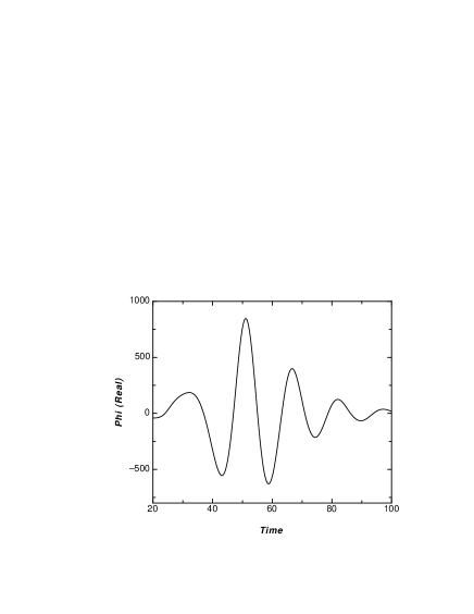
Figure 1: The quasi-normal ringing for a black hole with $a/M=0.9$; the $l=0$, $m=0$ mode is shown here. The evolution of the real part of the Teukolsky function, extracted at $r=20M$, $\theta=\pi/2$.

III Cell Broadband Engine

The CBE is a completely new processor, that was developed collaboratively by Sony, IBM and Toshiba primarily for multimedia applications. This processor has a general purpose (PowerPC) CPU, called the PPE (that can execute two (2) software threads simultaneously) and eight (8) special-purpose compute engines, called SPEs only for numerical computation. Each SPE can perform vector operations, which implies that it can compute on multiple data, in a single instruction (SIMD). All of these compute elements are connected to each other through a high-speed interconnect bus (EIB). A single 3.2 GHz CBE (original - 2006/2007) has a peak performance of over 200 GFLOP/s in single-precision floating point computation and 15 GFLOP/s in double-precision. The current (2008) release of the CBE, called the PowerXCell, has design improvements that bring the double-precision performance up to 100 GFLOP/s.

The main programming challenge introduced by this new design, is that one has to explicitly manage the memory transfer between the PPE and the SPEs. The PPE and SPEs are equipped with a DMA engine – a mechanism that enables data transfer to and from main memory and each other. Now, the PPE can access main memory directly, but the SPEs can only directly access their own, rather limited (256KB) local-store. This poses a challenge for many applications, including the NR application that we are considering in this article. However, the compilers in the most recent release (3.1) of IBM’s Cell SDK enable a software caching mechanism that allows for the use of the SPE local-store as a conventional cache, thus negating the need of transferring data manually from main memory. In essence, this mechanism allows one to write SPE programs that can access variables stored in the PPE’s address space (IBM refers this to as effective address space support). From our viewpoint, this feature takes away the main challenge associated to programming the CBE, and thus considerably reduces the amount of specialized code development needed. Therefore, we will take this approach in the development of a CBE optimized version of our NR application. Of course, it is worth pointing out that this approach will not allow the processor to perform at full potential; thus one should not expect to achieve the maximal performance gain that would be possible otherwise.

Another important mechanism that allows communication between the the different elements (PPE, SPEs) of the CBE is the use of mailboxes. These are special purpose registers that can be used for uni-directional communication. Each SPE has three (3) mailboxes – two (2) outbound, that can hold only a single entry, and one (1) inbound, that can hold four (4) entries. These are typically used for synchronizing the computation across the SPEs and the PPE, and that is primarily how we made use of these registers as well. Details on our specific use of these various aspects of the CBE for the NR application appear in the next section of this article.

IV CBE Teukolsky Code Implementation

As mentioned in the previous section, our approach towards running code on the Cell’s SPEs involves making use of the effective address space support. In this manner we avoid the involved programming associated to explicitly managing the data exchange between the PPE and the SPEs. Therefore, once we have decided upon the portion of the Teukolsky code that would be appropriate to run on the SPEs, the rest would be straightforward.

Since the SPEs are the main compute engines of the CBE, one would want them to execute the most compute intensive tasks of a code in a data- or task- parallel fashion, and leave the rest (input/output, synchronization, etc.) to run on the PPE. We employ a data-parallel model, which is straightforward to implement in a code like ours – we simply perform a domain decomposition of our finite-difference numerical grid and allocate the different parts of the grid to different SPEs. In particular, we parallelize along the $r^{*}$ coordinate dimension, because that typically has two orders-of-magnitude more grid points than the other ($\theta$) dimension.

Upon performing a basic profiling of our code using the GNU profiler gprof, we learn that the computing the “right-hand-sides” of the Lax-Wendroff steps i.e. the quantities within the square-brackets of Eqs. (II.2) and (14), take nearly 75% of the application’s overall runtime. Thus, it is natural to consider accelerating this “right-hand-side” computation using data-parallelization on the SPEs. We anticipate that this observation is fairly typical for codes of this type.

Now, to move this computation to the SPEs, we simply take the corresponding PPE code and copy it into a skeleton SPE code and then add in the appropriate declarations for all the field arrays such that they point to the corresponding quantities in the PPE’s address space. To be more explicit, lets say that we have a field array quantity phi defined in the PPE portion of the code as follows,

double phi[M][N];

where $M$ and $N$ are the dimensions of the array in the $\theta$ and $r^{*}$ directions respectively. To point to this exact same array from the SPE code, we simply need to declare it as,

extern __ea double phi[M][N];

where the __ea type qualifier is a PPE address namespace identifier. That entirely takes care of the complicated matter of transferring the necessary data back-and-forth between the SPEs and the PPE. Each SPE maintains a cache (size can be controlled at compile time using the -mcache-size flag) in its local-store, wherein it stores a small fraction of the whole array for immediate use; therefore its functioning is identical to the traditional hardware caches found in all modern processors.

Finally, as far as making use of the SIMD capabilities of the SPEs are concerned, we simply enable the auto-vectorizing capabilities of the spu-gcc compiler, as opposed to performing those optimizations by hand. The only other issue remaining, is that of synchronizing the PPE and the SPEs, which is easily done by using mailboxes as mentioned earlier.

V Performance Results

Recall that the “right-hand-side” computation, that we are coding for parallelized execution on the Cell’s SPEs takes nearly 75% of the overall runtime of the application. This means that at best, we can expect an acceleration of a factor of four (4) in the application’s overall runtime (Amdahl’s law). In this section, we compare our CBE accelerated code’s performance relative to this maximum achievable gain.

Fig. 2 depicts the total application runtime as a function of the number of SPEs used, for two (2) different values of the software cache. One can clearly see that although the performance gain using this approach is highly dependent on the size of the software cache used, the gains are substantial. For the case of the $128K$ cache size, the maximum acceleration of the application is a factor of $3.885$ – this translates to over 97% of the maximum theoretical gain possible through our parallel approach!

Another observation that can be made from the $128K$ cache data plotted in Fig. 2 is that after six (6) SPEs are in use, not much is gained by including additional SPEs. The reason for this is simply that even with only six (6) SPEs in use, the runtime associated to the “right-hand-side” computation becomes negligible as a fraction of the application’s overall runtime. Thus, including additional SPEs to further accelerate that computation yields no benefit. If we wanted to accelerate the application even further, we would need to further port some of the other PPE-based computations onto the SPEs.

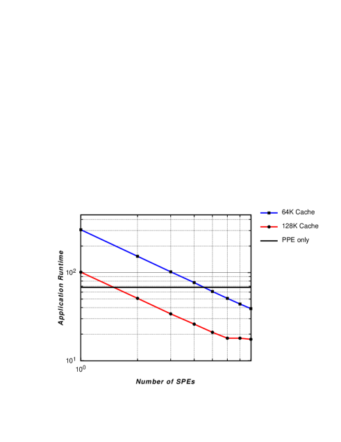
Figure 2: The overall application runtime of our CBE Teukolsky code, as a function of the number of SPEs used, for two (2) different software cache sizes. The performance gains owing to parallelization are significant, with more gain for larger cache size. We also depict the runtime of the PPE-only code for comparison purposes.

It is worth pointing out that these tests were performed on an IBM QS21 blade server that is equipped with the original (2006/2007) CBE – the one with the rather limited double-precision floating-point performance. All of our codes were run using double-precision floating-point accuracy because that is the common practice in the NR community and also a necessity for finite-difference based evolutions, especially if a large number of time-steps are involved. On the current PowerXCell processor, the overall performance of our code is likely to be much better.

VI Conclusions

We demonstrate that it is possible to obtain a significant performance gain (upto 97% of theoretical maximum) on a typical finite-difference PDE solver by making use of the SPEs of the Cell processor, via a programming model that is relatively very straightforward to implement. The approach involves the use of software caching through the recently made available effective address space support on the Cell’s SPEs.

By making use of this approach many scientific applications may obtain high accelerations on CBE hardware with minimal investment in detailed and specialized coding. Moreover, it is worth noting that we obtain these very strong results from the the original release of the Cell processor – the one found in the Sony PS3 – therefore, one can obtain these performance gains using such extremely low-cost hardware.

References

- (1) NVIDIA’s CUDA http://www.nvidia.com/cuda.
- (2) IBM’s Cell Broadband Engine project website http://www.research.ibm.com/cell.
- (3) Sony’s Playstation 3 gaming console website http://www.us.playstation.com/.
- (4) IBM’s QS21/22 Cell Broadband Engine blades http://www-03.ibm.com/systems/bladecenter.
- (5) IBM RoadRunner at Los Alamos National Lab http://www-03.ibm.com/systems/deepcomputing/rr/.
- (6) NSF LIGO laboratory http://ligo.caltech.edu.
- (7) G. Khanna et al., Inspiralling black holes: the close limit Phys. Rev. Lett. 83:3581–3584, 1999; L. Burko, G. Khanna, Radiative falloff in the background of rotating black hole, Phys. Rev. D 67:081502, 2003; L. Burko, G. Khanna, Universality of massive scalar field late-time tails in black-hole spacetimes, Phys. Rev. D 70:044018, 2004; M. Strafuss, G. Khanna, Massive scalar field instability in Kerr spacetime, Phys. Rev. D 71:024034, 2005; L. Burko, G. Khanna, Late-time Kerr tails revisited, Class. Quant. Grav. 26:015014, 2009.
- (8) S. Williams et al., Scientific computing kernels on the Cell processor, International Journal of Parallel Programming 35:263–298, 2007; M. Christen et al., Accelerating Stencil-Based Computations by Increased Temporal Locality on Modern Multi- and Many-Core Architectures, 2008.
- (9) Cell SDK http://www.ibm.com/developerworks/power/cell/.
- (10) Cactus Code http://www.cactuscode.org/.
- (11) S. Teukolsky, Perturbations of a rotating black hole, Astrophys. J. 185:635, 1973.
- (12) W. Krivan, P. Laguna, P. Papadopoulos, and N. Andersson, Dynamics of perturbations of rotating black holes, Phys. Rev. D 56:3395, 1997.