Tunable Berry curvature, valley and spin Hall effect in Bilayer MoS₂

Abstract

The chirality of electronic Bloch bands is responsible for many intriguing properties of layered two-dimensional materials. We show that in bilayers of transition metal dichalcogenides (TMDCs), unlike in few-layer graphene and monolayer TMDCs, both intra-layer and inter-layer couplings give important contributions to the Berry curvature in the $K$ and $-K$ valleys of the Brillouin zone. The inter-layer contribution leads to the stacking dependence of the Berry curvature and we point out the differences between the commonly available 3R type and 2H type bilayers. Due to the inter-layer contribution the Berry curvature becomes highly tunable in double gated devices. We study the dependence of the valley Hall and spin Hall effects on the stacking type and external electric field. Although the valley and spin Hall conductivities are not quantized, in MoS₂ 2H bilayers they may change sign as a function of the external electric field which is reminiscent of the behaviour of lattice Chern insulators.

I Introduction

The valley degree of freedom has recently attracted a large interest in monolayers of group-VI transition metal dichalcogenides (TMDCs). This is in good part due to the fact that monolayer TMDCs exhibit circular optical dichroism, that is, the valleys at the $\pm K$ point of the Brillouin zone (BZ) can be directly addressed by left or right circularly polarized lightCui ; Heinz ; Cao ; Urbaszek . A related phenomenon, called the valley-Hall effect, has also been demonstratedmonolayer-valleyH in monolayer MoS₂, which can be traced to the chirality of the electronic Bloch bandsDiXiao-valley ; WangYao-valley ; WangYao-TMDCmonolayer . The Berry curvatureBerry-phase-review properties of bilayer TMDCs have received very limited attention so farsymmetry-tuning , in part, due to the uncertainty about the position of the band edges in the Brillouin zone that one can find in the existing literaturemonolayer-valleyH ; DiXiao-valley ; WangYao-valley ; WangYao-TMDCmonolayer . A better understanding of the Berry curvature properties would be important in light of recent reportsvalley-Hall-BLMoS2 ; Morpurgo-3R-bilayer on the valley-Hall effect in bilayer MoS₂, and the purpose of this work is to analyse the topological properties of bilayer TMDCs (BTMDCs).

Because of the recent experimental progresssymmetry-tuning ; Iwasa ; Arita ; valley-Hall-BLMoS2 ; XiangSheng ; Morpurgo-3R-bilayer , we will concentrate on bilayer MoS₂ in the following, but many of our findings are equally valid for other BTMDCs such as MoSe₂, WS₂, and WSe₂. The focus of the present study is on the competition between the contributions towards Berry curvature of electron bands in BTMDCs coming from the intrinsic properties of the monolayers and a part generated by the inter-layer coupling. Thus, BTMDCs are markedly different from gapped bilayer graphene or monolayer TMDCs, where only one of the contributions is finiteWangYao-TMDCmonolayer ; Morpurgo-BLG . Because of the inter-layer contribution, the Berry curvature is tunable by moderately strong external electric fields. Moreover, we show that the stacking of the monolayer constituents in BTMDCs affects the Berry curvature and different stackings have Berry curvature properties. These topological differences can already be understood if spin-orbit coupling (SOC) is neglected. Nevertheless, we will also analyse the effect of SOC on the band structure, on the Berry curvature and on certain transport properties. The finite Berry curvature leads to valley and spin Hall conductivities which depend on the stacking and on the presence/absence of inversion symmetry in the system. As we will show below, the interplay of intrinsic SOC, the layer degree of freedom and an external electric field can lead to an interesting effect: the valley and spin Hall conductivities change sign as a function of the external electric field.

Generally, the presence/absence of inter/intra-layer Berry curvature contributions and the effect of different stacking is a relevant question for all layered materials, including, e.g., heterostructures of different monolayer TMDCs obtained by layer-by-layer growthAjayan or artificial alignmentTobiasKorn . BTMDCs, in addition, present a novel, rich playground for valley and spin related phenomena.

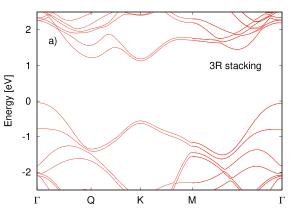
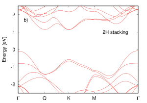
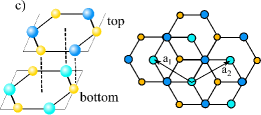
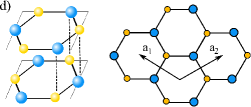
Figure 1: a) Band structure showing the CB and the VB of 3R stacked bilayer MoS₂ along the $\Gamma-K-M-\Gamma$ direction of the BZ from DFT calculations. b) The same for 2H stacked bilayer MoS₂. The spin-orbit coupling is neglected in a) and b). c) Schematic crystal structure of 3R stacked bilayer TMDCs in side view and in top view. d) Schematic crystal structure of 2H stacked bilayer TMDCs in side view, and in top view. In c) and d) the monolayers are shown as simple hexagonal lattices with two inequivalent sites, while $\mathbf{a}_{1}$ and $\mathbf{a}_{2}$ denote the lattice vectors.

II $\mathbf{k}\cdot\mathbf{p}$ Hamiltonian in the $\pm K$ valleys

There are two naturally occurring stable phases of bulk TMDCs with an underlying hexagonal symmetry of their lattice structureWilson . The most common one is the so-called 2H polytype, where the unit cell contains two monolayer units and the bulk is inversion symmetric. Some layered TMDCs, among others MoS₂, can also exist in the 3R polytype, where the unit cell contains three monolayers and inversion symmetry is broken in the bulk. Bilayer samples can be exfoliated from both bulk phases and we will refer to them as 2H and 3R stacked bilayers.

We start our discussion by introducing the $\mathbf{k}\cdot\mathbf{p}$ Hamiltonians for 3R and 2H stacked bilayers. We will focus on the $\pm K$ valleys in the BZ because in our DFT calculations [see Figures 1(a)-(b)] the band edge in the conduction band can be found at these point, therefore they are experimentally relevant. We will briefly discuss the $Q$ valleys in Section VI. The main differences between the Berry curvature properties of 3R and 2H bilayer TMDCs are orbital effects and therefore we neglect the SOC in the present Section. The discussion of the important effects of the SOC are deferred to Sections IV and V.

II.1 3R bilayers

We start our discussion with 3R stacked bilayer MoS₂, which can be exfoliated from the 3R bulk polytypeIwasa ; Arita ; XiangSheng ; Morpurgo-3R-bilayer . 3R bilayers are non-centrosymmetric (the symmetry of the crystal structure is described by the point group $C_{3v}$) and therefore, in contrast to 2H stacked bilayers (see below) one can expect interesting Berry curvature properties even if no external electric field is applied. We first introduce a $\mathbf{k}\cdot\mathbf{p}$ model for this system which differs in important details from the one used recently in Ref. Xiaoou, (see Appendix B.2 for the derivation of this model). The electronic properties at the $\pm K$ point of the BZ can be succinctly captured by the following simplified $\mathbf{k}\cdot\mathbf{p}$ Hamiltonian:

$$H^{3R}_{K}=\left(\begin{array}[]{cccc}\varepsilon_{cb}^{b}&\gamma_{3}\,q_{+}&\gamma_{cc}\,q_{-}&0\\ \gamma_{3}\,q_{-}&\varepsilon_{vb}^{b}&0&\gamma_{vv}\,q_{-}\\ \gamma_{cc}\,q_{+}&0&\varepsilon_{cb}^{t}&\gamma_{3}q_{+}\\ 0&\gamma_{vv}q_{+}&\gamma_{3}q_{-}&\varepsilon_{vb}^{t}\end{array}\right)$$ (1)

Here $q_{\pm}=\tau q_{x}\pm iq_{y}$ denotes the wavenumber measured from the $K$ (or $-K$) point of the BZ and $\tau=\pm 1$ is the valley index. Higher order terms in $q_{\pm}$, which appear in the $\mathbf{k}\cdot\mathbf{p}$ model of monolayer TMDCsPRB-paper ; Asgari ; 2DMaterials-paper have been neglected here. The band-edge energies of the CB and VB in the bottom (top) layers are denoted by $\varepsilon_{cb}^{b}$ ($\varepsilon_{cb}^{t}$) and $\varepsilon_{vb}^{b}$ ($\varepsilon_{vb}^{t}$). The layer index bottom (b) and top (t) are assigned to the bands based on the localization of the corresponding Bloch-wave function to one of the layers. We note that explicit density functional theory (DFT) wave function calculations for the bilayer case can be found in Ref. XiangSheng, , while for the bulk 3R polytype in Ref. Iwasa, . Our definition of the layer index is shown in Fig. 1(c): in the bottom monolayer the Mo atom does not have a S neighbour atom directly above it, while for the Mo atom in the top layer there is a S atom neighbour belonging to the bottom monolayer. Since in the monolayers the atomic Mo $d$ orbitals have the largest weight in the conduction and the valence band (CB and VB) at the $\pm K$ points one may expect that this difference in the atomic environment of the two Mo atoms can lead to different crystal field splittings in the two layers and hence it may affect the band structure of the bilayers. This is indeed what we can deduce from our DFT band structure calculations, i.e., that $\varepsilon_{cb\,(vb)}^{(b)}>\varepsilon_{cb\,(vb)}^{(t)}$, see also Appendix B.2. (We performed our DFT calculations using the VASP codeVASP , for further details see Ref. Viktor-DFT, ). Defining the band-edge energy differences $\delta E_{cc}=(\varepsilon_{cb}^{b}-\varepsilon_{cb}^{t})/2$ and $\delta E_{vv}=(\varepsilon_{vb}^{b}-\varepsilon_{vb}^{t})/2$, our DFT band structure calculations suggest that $\delta E_{cc}\neq\delta E_{vv}$, meaning that there is a small difference of about $10$ meV between the band gaps of the bottom and the top layer. This energy difference will be neglected in the following as this does not affect any of the main conclusions of the Berry curvature calculations. We denote therefore by $\delta E_{cc}=\delta E_{vv}:=\delta E_{ll}$ the inter-layer band-edge energy difference and use the notation $\delta E_{bg}=E_{bg}/2$ for half of the monolayer bandgap. We use $\gamma_{3}$ for the intra-layer coupling of the CB and VB, and $\gamma_{cc}$ ($\gamma_{vv}$) is the inter-layer couplings between the CBs (VBs) of the two monolayers. The numerical value of $\gamma_{3}$ can, in principle, be somewhat different in the two layers, but we neglect this effect and use the monolayer value. The coupling constants $\gamma_{cc}$ and $\gamma_{vv}$ can be estimated by fitting the eigenenergies of $H^{3R}_{K}$ to the DFT band structure (see Table 1). One can see from Eq. (1) that for $\mathbf{q}=0$ the two layers are decoupled, in agreement with previous resultsArita for the 3R bulk form.

II.2 2H bilayers

We now compare the results in Section II.1 with the corresponding ones for 2H stacked bilayer MoS₂ which derives from the 2H polytype [see Fig. 1(b)]. The $\mathbf{k}\cdot\mathbf{p}$ Hamiltonian reads

$$H^{2H}_{K}=\left(\begin{array}[]{cccc}\varepsilon_{cb}+U_{g}&\gamma_{3}\,q_{+}&\gamma_{cc}\,q_{-}&0\\ \gamma_{3}\,q_{-}&\varepsilon_{vb}+U_{g}&0&t_{\perp}\\ \gamma_{cc}\,q_{+}&0&\varepsilon_{cb}-U_{g}&\gamma_{3}q_{-}\\ 0&t_{\perp}&\gamma_{3}q_{+}&\varepsilon_{vb}-U_{g}\end{array}\right)$$ (2)

where $t_{\perp}$ is a momentum independent tunnelling amplitude between the VBs of the two layers and we included the possibility of an inter-layer potential difference given by $\pm U_{g}$, which can be induced by a substrate or an external electric field. A similar model, which neglected the coupling between the CBs, was introduced in Refs. WangYao-bilayer, ; symmetry-tuning, (see the Appendix B.1 for further details.) We will show, however, that the coupling between the CBs gives an important contribution to the Berry curvature. For $U_{g}=0$ the system is inversion symmetric (the crystal symmetries are described by point group $D_{3d}$). At the $\pm K$ points the two CBs are degenerate, while the VBs are split due to the tunnelling amplitude $t_{\perp}$ [see Fig. 1(b)]. Away from the $\pm K$ points the CBs are also split, for small $\mathbf{q}$ wavenumbers this splitting is mainly due to the interlayer coupling term $\gamma_{cc}q_{\pm}$.

III Berry curvature of BTMDCs

III.1 Numerical results and analytical approach

The Berry curvature of band $n$ in a 2D material is defined by $\Omega_{z}(\mathbf{k})=\nabla_{\mathbf{k}}\times i\langle u_{n,\mathbf{k}}|\nabla_{\mathbf{k}}u_{n,\mathbf{k}}\rangle$, where $u_{n,\mathbf{k}}$ is the lattice-periodic part of the Bloch wave functions. In the envelope function approximation $u_{n,\mathbf{k}}$ can be calculated from a $\mathbf{k}\cdot\mathbf{p}$ Hamiltonian valid around a certain $\mathbf{k}$-space point. Using the $\mathbf{k}.\mathbf{p}$ models introduced in Sections II.1 and II.2, in the $\pm K$ valleys the $u_{n,\mathbf{k}}$ functions are 4-spinors that can be obtained by e.g., numerically diagonalizing $H^{3R}_{K}$ and $H^{2H}_{K}$ of Eqs. (1) and (2), respectively. We used these eigenstates and the approach introduced by Ref. Fukui, to calculate the Berry curvature. The $\Omega_{z}(\mathbf{k})$ obtained for 3R and 2H bilayers is shown in Figures 2(a) and (b), respectively (the material parameters used in these calculations are given in Table 1). For comparison, we also show the Berry curvature that can be obtained from a gapped-graphene modelWangYao-TMDCmonolayer which approximately describes the band structure of individual monolayers in the limiting case when all inter-layer coupling terms in Eqs. (1) and (2) are neglected. It is clear that the Berry curvature of both types of bilayer is substantially different from the monolayer case suggesting that inter-layer coupling may have an important role.

To show this explicitly, we now derive an approximation for $\Omega_{z}(\mathbf{k})$ which can make analytical calculations easier. As it is well known, one can use the Schrieffer-Wolff transformationWinkler-book $e^{-S}He^{S}$ of a Hamiltonian $H$ to eliminate coupling terms between subsystems of $H$ in order to obtain an effective Hamiltonian $\tilde{H}$ in the desired subspace. Here $S=-S^{\dagger}$ is an anti-Hermitian operator. Denoting the eigenfunctions of $\tilde{H}$ by $\tilde{\Psi}$, the eigenfunctions $\Psi$ of the original Hamiltonian $H$ can be obtained by a back-transformation $\Psi=e^{S}\tilde{\Psi}$. By writing $e^{S}=\mathbb{1}+S+\frac{1}{2!}S^{2}+\dots$ a systematic approximation of $\Psi$ can be obtained if $\tilde{\Psi}$ is known. By using this approximation for $\Psi$ in the expression of $\Omega_{z}$, one finds

$$\Omega_{z}(\mathbf{k})=\nabla_{\mathbf{k}}\times i\left\{\langle\tilde{\Psi}|\nabla_{\mathbf{k}}\tilde{\Psi}\rangle+\frac{1}{2}\langle\tilde{\Psi}|[\nabla_{\mathbf{k}}S,S]|\tilde{\Psi}\rangle+\dots\right\}$$ (3)

where $[A,B]$ denotes the commutator of $A$ and $B$. Although $S$ is usually not known exactly, one can write $S=S^{(1)}+S^{(2)}+\dots$ and explicit expressions for $S^{(i)}$ can be found in e.g., Ref. Winkler-book, . In this way Eq. (3) can be used to obtain a perturbation series for $\Omega_{z}$. One may write $\Omega_{z}\approx\Omega_{z}^{(0)}+\Omega_{z}^{(1,1)}+\dots$ where $\Omega_{z}^{(0)}=\nabla_{\mathbf{k}}\times i\langle\tilde{\Psi}|\nabla_{\mathbf{k}}\tilde{\Psi}\rangle$ and $\Omega_{z}^{(1,1)}=\nabla_{\mathbf{k}}\times\frac{i}{2}\langle\tilde{\Psi}|[\nabla_{\mathbf{k}}S^{(1)},S^{(1)}]|\tilde{\Psi}\rangle$.

III.2 Berry curvature of 3R and 2H bilayers

In the case of 3R bilayers one may choose as a subspace e.g., one of the layers and treat the inter-layer coupling as perturbation. This corresponds to neglecting the inter-layer coupling in the wave function but retaining it in $S^{(1)}$. Using Eq. (3) we find that $\Omega_{z}^{(b)}$ ($\Omega_{z}^{(t)}$) for the bottom (top) layer can be written as $\Omega_{z}^{(b)}\approx\Omega_{z}^{(0)}-\Omega_{z}^{(1,1)}$ ($\Omega_{z}^{(t)}\approx\Omega_{z}^{(0)}+\Omega_{z}^{(1,1)}$), where

$$\Omega_{z}^{(0)}(\mathbf{q})=\pm\frac{\tau}{2}\left(\frac{\gamma_{3}}{\delta E_{bg}}\right)^{2}\frac{1}{\left(1+\left(\frac{\gamma_{3}|\mathbf{q}|}{\delta E_{bg}}\right)^{2}\right)^{3/2}},$$ (4a)

$$\Omega_{z}^{(1,1)}(\mathbf{q})\approx\frac{\tau}{(2\delta E_{ll})^{2}}\left(\lambda_{1}\pm\frac{\lambda_{2}}{\left(1+\left(\frac{\gamma_{3}|\mathbf{q}|}{\delta E_{bg}}\right)^{2}\right)^{1/2}},\right)$$ (4b)

Here $|\mathbf{q}|$ is the magnitude of $\mathbf{q}$, $\lambda_{1}=\gamma_{cc}^{2}+\gamma_{vv}^{2}$, $\lambda_{2}=\gamma_{cc}^{2}-\gamma_{vv}^{2}$ and the $+$ ($-$) sign corresponds to the CB (VB). $\Omega_{z}^{(0)}$ in Eq. (4a) is the well known result for a gapped-graphene two-band modelBerry-phase-review ; WangYao-valley , while Eq. (4b) is a correction due to the inter-layer coupling. The first correction to Eq. (4b) is $\sim\mathbf{q}^{2}$ but we found that for the wavenumber range of interest it is quite small.

In 2H bilayers, if both inversion and time reversal symmetries are simultaneously present, $\Omega_{z}$ vanishesBerry-phase-review . However, a finite inter-layer potential $\pm U_{g}$ breaks inversion symmetry, opens a gap in the CB at the $\pm K$ point, and causes $\Omega_{z}(\mathbf{q})$ to be non-zero. For the physically relevant case of $U_{g}\ll\delta E_{bg}$ it proves to be useful to treat the intra-layer coupling between the CB and VB in each layer as a perturbation that enters $S^{(1)}$. Following the same steps as for the 3R stacking, one finds that in the CB the Berry curvature is given by $\Omega_{z,cb}=\Omega_{z,cb}^{(0)}+\Omega_{z,cb}^{(1,1)}$, where

$$\Omega_{z,cb}^{(0)}(\mathbf{q})=\mp\frac{\tau}{2}\frac{\gamma_{cc}^{2}U_{g}}{\left(U_{g}^{2}+\left({\gamma_{cc}|\mathbf{q}|}\right)^{2}\right)^{3/2}}\\$$ (5a)

is due to the inter-layer coupling of the CBs. The second contribution reads

$$\Omega_{z,cb}^{(1,1)}(\mathbf{q})\approx\pm\frac{\tau}{2}\left(\frac{\gamma_{3}}{\delta E_{bg}}\right)^{2}\lambda_{3}\frac{U_{g}}{\left(U_{g}^{2}+\left({\gamma_{cc}|\mathbf{q}|}\right)^{2}\right)^{1/2}},$$ (5b)

where, using the notation $\tilde{\varepsilon}_{vb}=\sqrt{t_{\perp}^{2}+U_{g}^{2}}$, the constant $\lambda_{3}$ is given by $\lambda_{3}=1+\frac{3}{4}\left(\frac{\tilde{\varepsilon}_{vb}}{\delta E_{bg}}\right)^{2}$ and terms $\sim\mathbf{q}^{2}$ have been neglected in Eq. (5b). $\Omega_{z,cb}^{(1,1)}(\mathbf{q})$ is non-zero even if we set $\gamma_{cc}=0$, i.e., this term describes a Berry curvature contribution due to the intra-layer coupling of the CB and the VB. For the VB one finds that $\Omega_{z,vb}^{(0)}=0$ and the first non-zero term is

$$\Omega_{z,vb}^{(1,1)}=\mp 2\tau\frac{\gamma_{3}^{2}U_{g}}{\tilde{\varepsilon}_{vb}(E_{bg}\mp\tilde{\varepsilon}_{vb})^{2}},$$ (6)

which is in agreement with Ref. symmetry-tuning, for $\tilde{\varepsilon}_{vb}\ll E_{bg}$. This means that the Berry curvature is, in first approximation, dispersionless in the VB. The upper (lower) sign in Eqs. (5a)-(5b) and (6) corresponds to the bands that have larger weight in the layer at $+U_{g}$ ($-U_{g}$) potential. One can note that the inter-layer ($\Omega_{z,cb}^{(0)}$) and intra-layer ($\Omega_{z,cb}^{(1,1)}$) contributions have opposite sign in each valley. As shown in Figures 2(a) and (b), our numerical calculations using the eigenstates of Eq. (1) and (2) are in good agreement with the analytical results of Eqs. (4b) and Eqs. (5b)-(6).

III.3 Discussion

One can see that although the band structure of 3R and 2H stacked bilayers look rather similar, especially in the valence band [c.f. Figures 1(a) and 1(b)], the comparison of Figs. 2(a) and 2(b) reveals several important differences between their Berry curvature properties. Considering first the 3R bilayers, the Berry curvature is essentially layer-coupled both in the VB and in the CB: it is significantly larger in the CB of the top layer than of the bottom layer, while the converse is true for the VBs [see Fig. 2(a)]. In the CB of the bottom and top layers one finds for $\mathbf{q}=0$ that $\Omega_{z,cb}=\Omega_{z,cb}^{(0)}+\Omega_{z,cb}^{(1,1)}=\frac{\tau}{2}[(\gamma_{3}/\delta E_{bg})^{2}\mp(\gamma_{cc}/\delta E_{ll})^{2}]$, where $-$ $(+)$ sign is for the bottom (top) layer. This expression shows that i) both intra-layer and inter-layer coupling contribute to the Berry curvature, and (ii) the two contributions can either reinforce or weaken each other. The effect of the inter-layer coupling is clearly visible: it reduces $\Omega_{z,cb}$ for the bottom layer and enhances it for the top layer. A similar but opposite effect takes place in the VB as well, where $\Omega_{z,vb}=-\frac{\tau}{2}[(\gamma_{3}/\delta E_{bg})^{2}\pm(\gamma_{vv}/\delta E_{ll})^{2}]$. Using the band-structure parameters given in Table 1, we find that the intra-layer and the inter-layer contributions are of similar magnitude: although the coupling $\gamma_{cc}$ between the layers is much weaker than the intra-layer coupling $\gamma_{3}$ between the CB and the VB, since $\delta E_{ll}\ll\delta E_{bg}$, the ratios $\gamma_{3}/\delta E_{bg}$ and $\gamma_{cc}/\delta E_{ll}$ are of the same order of magnitude. This conclusion does not seem to depend on the level of theory applied in the first-principles calculations which yield the band-structure parameters for the $\mathbf{k}\cdot\mathbf{p}$ theory: using, as an estimate, the parametrization for $\gamma_{3}$ and $\delta E_{bg}$ of e.g., Ref. Kaxiras, which are based on GW calculations for the 2H polytype, one still finds that the ratio $\gamma_{3}/\delta E_{bg}$ is similar in the DFT and GW calculations and we expect the same for $\gamma_{cc}/\delta E_{ll}$. Moreover, $\Omega_{z}^{(1,1)}$ and hence the total Berry curvature may be tunable by an external electric field which would change $\delta E_{ll}$. We point out that the external electric field can, in principle, both decrease and increase $\delta E_{ll}$ depending on its polarity, and the same can be expected for $\Omega_{z}^{(1,1)}$ as well (assuming that $\gamma_{cc}$ and $\gamma_{vv}$ do not change significantly). While $E_{bg}$ and hence $\Omega_{z}^{(0)}$ is difficult to change by electric field because it depends on the crystal field splitting of the atomic Mo $d$ orbitals, $\delta E_{ll}$ is determined by weaker inter-layer interactions and hence it might be more easily tunable.

For 2H bilayers, on the other hand, the Berry curvature is CB-coupled: it is much larger in the CB than in the VB [see Fig. 2(b)]. This can be understood from Eqs. (5a) and (5b): for small $\mathbf{q}$ values, such that $\gamma_{cc}|\mathbf{q}|<<U_{g}$ the main contribution to $\Omega_{z,cb}$ comes from the inter-layer term $\Omega_{z,cb}^{(0)}$ and can be quite large for small $U_{g}$ values. Similarly to 3R bilayers, therefore, $\Omega_{z,cb}$ is gate tunable. In contrast, using Eq. (6) we expect that the Berry curvature, albeit gate tunable, will be rather small in the VB. Assuming $U_{g}$ of the order of $1-10$ meV which we think is experimentally feasible, one finds that $U_{g}$ is significantly smaller than $t_{\perp}$ (see Table 1) and therefore $\Omega_{z,vb}^{(1,1)}\sim 0.5-1.0$ Ų.

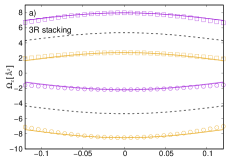
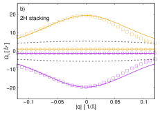
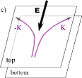
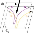
Figure 2: Comparison of numerical and analytical calculation of $\Omega_{z}$ around the $K$ point for a) 3R stacked, and b) 2H stacked bilayer MoS₂. $\square$ show the results for CBs, $\bigcirc$ for VBs. In a), brown colour corresponds to bands in the bottom layer, purple to bands in the top layer, solid lines show the results of Eq. (4b). Dashed lines indicate the Berry curvature $\Omega_{z}^{(0)}$ of a monolayer, given by Eq. (4a). In b) brown colour corresponds to the layer at $-U_{g}$, purple to the layer at $+U_{g}$ potential, solid lines show the results of Eqs. (5a)-(5b) and (6), dashed lines indicate $\Omega_{z,cb}^{(0)}$ for the inter-layer contribution given by Eq. (5a). For material parameters of the $\mathbf{k}\cdot\mathbf{p}$ models see Table 1. In b) we used $U_{g}=10$meV. The plotted range corresponds to around 10% of the $\Gamma-K$ distance in the BZ. c) and d): Schematics of the valley Hall conductivity contributions in the CB of 3R and 2H bilayers, respectively, when an in-plane electric field $\mathbf{E}$ is applied.

	$t_{\perp}$ [eV]	$\gamma_{cc}$ [eVÅ]	$\gamma_{vv}$ [eVÅ]	$\delta E_{cc}$ [eV]	$\delta E_{vv}$ [eV]
3R	-	$0.0708$	$0.0779$	$0.029$	$0.033$
2H	$0.045$	$0.0706$	-	-	-

Table 1: Material parameters obtained by fitting the DFT band structure calculations which do not take into account SOC, using Eqs. (1) and (2). To obtain Figs. 2(a) and (b) we used $\gamma_{3}=2.73$ eVÅ  and $E_{bg}=1.67$eV from Ref. 2DMaterials-paper, and $\delta E_{ll}=0.031$eV.

IV Spin-orbit coupling effects

The considerations in Sections II and III should be applicable to all homobilayer TMDCs. We have not yet discussed the effect of the spin-orbit coupling (SOC) on the Berry curvature properties of BTMDCs. Generally, the SOC in BTMDCs is more complex than in monolayers, see the Appendices B.1.2 and B.2.2 for details. Moreover, in 3R bilayers the low-energy physics also depends on the ratio of the band-edge energy difference $\delta E_{cc}$ and $\delta E_{vv}$ and the monolayer SOC coupling strengths $\Delta_{cb}$ and $\Delta_{vb}$. These energy scales can be quite different in different BTMDCs. Because of the recent experimental activityvalley-Hall-BLMoS2 ; Morpurgo-3R-bilayer we will focus on bilayer MoS₂. Our DFT calculations suggest that for bilayer MoS₂ it is sufficient to take into account only the intrinsic SOC of the constituent monolayers.

IV.1 3R bilayer MoS₂

Fig. 3(a) shows the band structure of 3R bilayer MoS₂ obtained from DFT calculations. In contrast to Fig. 1(a) here the SOC is also taken into account. The effects of the SOC at the $K$ point of the BZ are highlighted by comparing the schematic band structure without and with the SOC in Figs. 3(c) and 3(d), respectively. As already explained in Section II, the band edge energy is different for bands localized to the top and bottom layers both in the CB and the VB. Upon considering the SOC, since 3R bilayers lack inversion symmetry, their bands, apart from the $\Gamma-M$ direction in the BZ, will be spin-orbit split and spin-polarized [Fig. 3(a)]. The SOC is diagonal in the layer index and it can be described by adding a term $H_{so,cb}^{3R}=\Delta_{cb}\tau_{z}s_{z}$ ($H_{so,vb}^{3R}=\Delta_{vb}\tau_{z}s_{z}$) to the CB (VB) of the constituent monolayers, where $\Delta_{cb(vb)}$ is (in good approximation) the SOC strength in monolayer MoS₂, $s_{z}$ is a spin Pauli matrix and the Pauli matrix $\tau_{z}$ acts in the valley space. Our DFT calculations show that $\Delta_{cb}$ is much smaller than the inter-layer band-edge energy difference $\delta E_{cc}$. Therefore, as shown schematically in Fig. 3(d), it has a minor effect on the band structure. The situation is different in the VB, because $\Delta_{vb}$ is larger than the band-edge energy difference $\delta E_{vv}$. Therefore in the $\pm K$ valleys the four highest energy spin-split VB show an alternating layer polarization pattern.

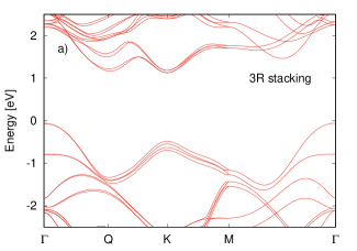
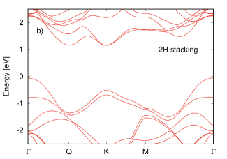
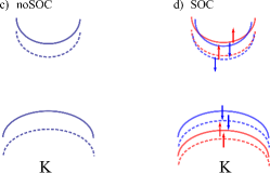
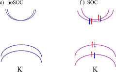
Figure 3: SOC effects in the band structure of bilayer MoS₂. a) DFT band structure calculations along the $\Gamma-K-M-\Gamma$ line of the BZ for 3R bilayer. b) The same as in a) for 2H bilayer. c) For 3R bilayers, close to the $\pm K$ points the layer index is an approximately good quantum number for each of the bands both in the CB and the VB. Neglecting the SOC (noSOC) the lowest CB is mostly localized to the top layer (dashed line), while the next CB band (solid line) to the bottom layer. The opposite is true for the two highest energy VBs. The bands are shifted in energy due to the inter-layer band edge energy difference $2\delta E_{cc}$ and $2\delta E_{vv}$. d) When SOC is taken into account for 3R bilayers, each of the bands becomes spin-split and spin polarized. Red corresponds to $\uparrow$, blue to $\downarrow$ spin polarization. The spin-splitting $\Delta_{cb}$ of the two lowest CBs is much smaller than the inter-layer splitting $\delta E_{cc}$. The situation is different for the VBs: here $\Delta_{vb}\gtrsim\delta E_{vv}$ and therefore the spin-polarized bands have an alternating layer index. e) For 2H bilayers, if SOC is neglected (noSOC), the two lowest energy CB are degenerate at the $\pm K$ points and weakly split due to the inter-layer coupling away from the $\pm K$ points. The energy splitting of the two highest energy VBs is $2t_{\perp}$. Both layers contribute with equal weight to each of the bands. f) When SOC is taken into account for 2H bilayers, in the CB there are two two-fold degenerate and spin-unpolarized bands separated by an energy $2\Delta_{cb}$ at the $\pm K$ point. A combined layer and spin index can be assigned to each of the four CB bands at the $\pm K$ point, away from the $\pm K$ points both layers contribute to each of the bands, but with different weights. In the VB both layers contribute to each of the bands, even at the $\pm K$ points. Only if $\Delta_{vb}\gg t_{\perp}$ do the bands become approximately layer polarizedWangYao-bilayer . In d) and f) the spin-polarization of the bands in the $-K$ valley can be obtained by taking the time reversed states.

Regarding the Berry curvature calculations, the effect of SOC on the formulas Eqs. (4b) can be rather straightforwardly taken into account by introducing the spin-dependent band gaps $\delta E_{bg}^{\downarrow}=\delta E_{bg}-\tau(\Delta_{cb}+\Delta_{vb})/2$ and $\delta E_{bg}^{\uparrow}=\delta E_{bg}+\tau(\Delta_{cb}+\Delta_{vb})/2$ and the corresponding spin-dependent Berry curvatures for the top and bottom layers. Note that $\delta E_{ll}$ in Eq. (4b) is not affected by the SOC because in 3R bilayers, unlike in 2H bilayers, the SOC is not layer dependent and therefore it drops out from the inter-layer energy difference.

IV.2 2H bilayer MoS₂

Turning now to the 2H bilayers, we remind that if SOC is neglected and inversion symmetry is not broken, the CB is doubly degenerate, while the VB is non-degenerate in the $\pm K$ point [Fig. 1(b)]. If now spin is taken into account but SOC is neglected, this would mean a four-fold degeneracy of the CB. However, the SOC partially lifts this four-fold degeneracy and leads to two two-fold degenerate levels, see Figs. 3(e) and 3(f). In contrast to the 3R bilayers, due to the inversion symmetry all bands of 2H bilayers remain spin-degenerate even when SOC is considered. The SOC of 2H bilayers can be described by the Hamiltonian $H_{so,cb}^{2H}=\Delta_{cb}\tau_{z}\sigma_{z}s_{z}$ ($H_{so,vb}^{2H}=\Delta_{vb}\tau_{z}\sigma_{z}s_{z}$) in the CB (VB) of the bilayer. Here the Pauli matrix $\sigma_{z}$ indicates that within a given valley the SOC has a different signWangYao-bilayer in the two layers: this can be understood from the fact that the layers are rotated by $180^{\circ}$ with respect to each other. At each energy there will be a $\uparrow$ and a $\downarrow$ polarized band, see Fig. 3(f). In the CB the splitting between the two-fold degenerate levels is essentially given by the SOC strength $2\Delta_{cb}$ of monolayer TMDCs. In the VB the main effect of the SOC is to increase the energy splitting of the two highest bands from $2t_{\perp}$ to $2\sqrt{\Delta_{vb}^{2}+t_{\perp}^{2}}$.

The SOC has an interesting effect on the Berry curvature. Considering first the CB, the SOC leads to a finite $\Omega_{z,cb}^{(0)}$ even for $U_{g}=0$, i.e., when there is no external electric field applied. The corresponding formulas can be obtained from Eqs. (5a), (5b) by making the substitution $U_{g}\rightarrow\Delta_{cb}$ and using $\tilde{\varepsilon}_{vb}=\sqrt{\Delta_{vb}^{2}+t_{\perp}^{2}}$ in the expression for $\tilde{\lambda}_{3}$. One can label $\Omega_{z}$ by a spin index $s=\uparrow,\downarrow$ and write $\Omega_{z,cb}^{\uparrow}=\Omega_{z,cb}^{(0)}+\Omega_{z,cb}^{(1,1)}$, where the upper (lower) sign appearing in Eqs. (5a) and (5b) corresponds to the band at energy $\varepsilon_{cb}+\tau\Delta_{cb}$ ($\varepsilon_{cb}-\tau\Delta_{cb}$) for $\mathbf{q}=0$. Regarding the $\downarrow$ bands, one finds $\Omega_{z,cb}^{\downarrow}=-\Omega_{z,cb}^{\uparrow}$. In the VB, for the physically relevant spin-degenerate band at the band gap one finds

$$\Omega_{z,vb}^{(1,1,s)}=\tau\cdot s\frac{2\gamma_{3}^{2}\Delta_{vb}}{\tilde{\varepsilon}_{vb}(E_{bg}-\tilde{\varepsilon}_{vb})^{2}},$$ (7)

where $s=1$ for the $\uparrow$ ($s=-1$ for $\downarrow$) spin-polarized band. This result was also obtained in Ref. WangYao-bilayer, .

V Valley Hall effects

We now discuss how the Berry curvature affects the valley and spin Hall conductivities in bilayer MoS₂. Since few-layer MoS₂ on dielectric substrate is often found to be $n$-dopedTartakovskii , we will focus on the valley Hall effects in the CB. Although the Q and K valleys are nearly degenerate, in our DFT calculations the band edge in the CB is at the $\pm K$ point. Therefore we can use the results obtained in Sections III and IV. The relevance of the $Q$ point valleys in the CB will be briefly discussed in Section VI. Regarding the VB, we briefly note that the band edge energy difference $E_{\Gamma K}$ between the $\Gamma$ and $K$ points is quite large, $500-600$ meV and therefore the $K$ valley is not relevant for transport properties of $p$-doped samples. Nevertheless, in other BTMDCs $E_{\Gamma K}$ might be much smallerFranchini ; Mauri than in MoS₂ and therefore the $\pm K$ valleys may also play an important role. We leave the study of the valley Hall effect in the VB of BTMDCs to a future work.

Due to the Berry curvature, if an in-plane electric field is applied, the charge carriers will acquire a transverse anomalous velocity componentBerry-phase-review which gives rise to an intrinsic contribution to the Hall conductivityAnomalousHall-review . We may define the valley Hall conductivity $\sigma_{v,H}$ of band $n$ asWangYao-TMDCmonolayer ; AnomalousHall-review

$$\sigma_{n,v,H}=\frac{e^{2}}{\hbar}\int\frac{d\mathbf{q}}{(2\pi)^{2}}\left[f_{n}^{\uparrow}(\mathbf{q})\Omega_{z,n}^{\uparrow}(\mathbf{q})+f_{n}^{\downarrow}(\mathbf{q})\Omega_{z,n}^{\downarrow}(\mathbf{q})\right]$$ (8)

where $f_{n}^{\uparrow,\downarrow}(\mathbf{q})$ is the Fermi-Dirac distribution function. Similarly, the spin Hall conductivity can be defined as

$$\sigma_{n,s,H}=\int\frac{d\mathbf{q}}{(2\pi)^{2}}\left[f_{n}^{\uparrow}(\mathbf{q})\Omega_{z,n}^{\uparrow}(\mathbf{q})-f_{n}^{\downarrow}(\mathbf{q})\Omega_{z,n}^{\downarrow}(\mathbf{q})\right].$$ (9)

Since we only study the valley Hall effects in the CB, we neglect the band index $n$ in the following. For later reference we note that since for each band one may write the Berry curvature as $\Omega_{z}=\Omega_{z}^{(0)}+\Omega_{z}^{(1,1)}$, the corresponding conductivities read $\sigma_{v,H}=\sigma_{v,H}^{(0)}+\sigma_{v,H}^{(1,1)}$ and $\sigma_{s,H}=\sigma_{s,H}^{(0)}+\sigma_{s,H}^{(1,1)}$.

V.1 3R bilayers

Due to the relatively large band-edge energy difference $2\delta E_{ll}=58$ meV, for typical $n$-doping only the CB (mostly) localized to the top layer would be occupied and have a finite $\sigma_{v,H}$ and $\sigma_{s,H}$ contribution [the former is shown schematically in Fig. 2(c)]. This situation is similar to one of the proposed strongly interacting phases of bilayer graphene, namely, to the Quantum Valley Hall insulator phaseBLG-Hallstates . However, in our case $\sigma_{v,H}$ is not quantized. In the following we assume that the charge density is large enough so that both spin-split CB bands in the top layer are populated and we add up their contributions to $\sigma_{v,H}$ and $\sigma_{s,H}$. Since $\Omega_{z}(\mathbf{q})$ changes rather slowly around the $\pm K$ points [see Fig. 2(a)] we may use $\Omega_{z}(\mathbf{q}=0)$ in Eq. (8) and at zero temperature one finds

$$\sigma_{v,H}^{3R} =\frac{\tau}{2}\frac{e^{2}}{\hbar}\left[\left(\frac{\gamma_{cc}}{\delta E_{cc}}\right)^{2}\frac{q_{F,\downarrow}^{2}+q_{F,\uparrow}^{2}}{4\pi}\right.$$ (10)

$$+\left.\left(\frac{\gamma_{3}}{\delta E_{bg}^{\uparrow}}\right)^{2}\frac{q_{F,\uparrow}^{2}}{4\pi}+\left(\frac{\gamma_{3}}{\delta E_{bg}^{\downarrow}}\right)^{2}\frac{q_{F,\downarrow}^{2}}{4\pi}\right]$$

where $q_{F,\downarrow}$ ($q_{F,\uparrow}$) is the Fermi wavevector for electrons of $\downarrow$ ($\uparrow$) spin. The term in the first line on the right-hand-side (r.h.s) of Eq. (10) corresponds to $\sigma_{v,H}^{(1,1)}$ while the second line is $\sigma_{v,H}^{(0)}$. One may recognize that $\sigma_{v,H}^{(0)}$ equals the valley Hall conductivity $\sigma_{v,H}^{ml}$ of monolayer TMDCsWangYao-TMDCmonolayer . Note that $(q_{F,\downarrow}^{2}+q_{F,\uparrow}^{2})/{4\pi}=n_{e,v}$ is the total charge density per valley. After expanding the second line of Eq. (10) in terms $(\Delta_{cb}+\Delta_{vb})/(2\delta E_{bg})$, one finds that it is also $\sim n_{e,v}$ plus a correction $\sim(q_{F,\uparrow}^{2}-q_{F,\downarrow}^{2})$ which is typically small with respect to terms that are $\sim n_{e,v}$. Since $\gamma_{3}/\delta E_{bg}$ and $\gamma_{cc}/\delta E_{ll}$ are of the same order of magnitude, Eq. (10) shows that $\sigma_{v,H}^{3R}$ is roughly twice as big as $\sigma_{v,H}^{ml}$. The sign of $\sigma_{v,H}^{3R}$ is opposite in the $K$ and $-K$ valleys, therefore no net bulk charge current flows unless there is a charge imbalance between the valleys. Calculating the spin Hall conductivity e.g., in the $K$ valley, it reads

$$\sigma_{s,H}^{3R} =\frac{1}{2}\left[\left(\frac{\gamma_{cc}}{\delta E_{cc}}\right)^{2}\frac{q_{F,\uparrow}^{2}-q_{F,\downarrow}^{2}}{4\pi}\right.$$ (11)

$$+\left.\left(\frac{\gamma_{3}}{\delta E_{bg}^{\uparrow}}\right)^{2}\frac{q_{F,\uparrow}^{2}}{4\pi}-\left(\frac{\gamma_{3}}{\delta E_{bg}^{\downarrow}}\right)^{2}\frac{q_{F,\downarrow}^{2}}{4\pi}\right].$$

The second line in Eq. (11), which corresponds to $\sigma_{s,H}^{(0)}$, is the same as in monolayer MoS₂. Because of the $\sigma_{s,H}^{(1,1)}$ contribution shown in the first line on the r.h.s of Eq. (11), $\sigma_{s,H}^{3R}$ is larger than $\sigma_{s,H}^{ml}$ in monolayer MoS₂. The term $q_{F,\uparrow}^{2}-q_{F,\downarrow}^{2}$ can be expressed as $(q_{F,\uparrow}^{2}-q_{F,\downarrow}^{2}){}=\frac{2(m_{\uparrow}-m_{\downarrow})}{\hbar^{2}}E_{F}+\frac{2m_{\uparrow}}{\hbar^{2}}\Delta_{cb}$ where $m_{\uparrow}$ and $m_{\downarrow}$ are the effective masses of the spin-split bands. Therefore the enhancement of $\sigma_{s,H}^{3R}$ depends on the Fermi energy $E_{F}$ and on $\Delta_{cb}$. Our DFT calculations suggest that in MoS₂ the term $\frac{2m_{\uparrow}}{\hbar^{2}}\Delta_{cb}$ would dominate for $E_{F}\lesssim$ few tens of meV because $m_{\uparrow}-m_{\downarrow}\approx 0.03m_{e}$ is rather small (here $m_{e}$ is the free electron mass). As we discussed for $\sigma_{v,H}^{3R}$, $\sigma_{s,H}^{(0)}$ can be expanded in terms of $(\Delta_{cb}+\Delta_{vb})/(2\delta E_{bg})$ and we find that $\sigma_{s,H}^{3R}$ is roughly twice as big as $\sigma_{s,H}^{ml}$. One can also easily show that, as in monolayersWangYao-TMDCmonolayer , the magnitude and sign of $\sigma_{s,H}^{3R}$ does not depend on the valley index $\tau$.

V.2 2H bilayers

The situation is more complex for 2H bilayers than for their 3R counterparts. As a first step we will discuss the valley Hall and spin Hall effects qualitatively. Let us start with the $U_{g}=0$ case. As already mentioned in Section IV, the SOC leads to a finite Berry curvature even for $U_{g}=0$. Since inversion symmetry is not broken and therefore each band is spin-degenerate, $f_{n}^{\downarrow}(\mathbf{q})=f_{n}^{\uparrow}(\mathbf{q})$. On the other hand, one finds that $\Omega_{z}^{\uparrow}(\mathbf{q})=-\Omega_{z}^{\downarrow}(\mathbf{q})$ and therefore $\sigma_{v,H}^{2H}$ vanishes in this limit. However, $\Omega_{z}^{\uparrow}(\mathbf{q})-\Omega_{z}^{\downarrow}(\mathbf{q})$, and hence $\sigma_{s,H}$ are non-zero. This is allowed because both the (in-plane) electric field and the spin current transform in the same way under time-reversal and inversion symmetriesMurakami .

In general, for $U_{g}>0$ both $\sigma_{v,H}^{2H}$ and $\sigma_{s,H}^{2H}$ will be finite. For concreteness, we consider the $K$ point and first discuss qualitatively the evolution of the band structure and the valley Hall conductivity as a function of $U_{g}$. The finite interlayer potential difference leads to the breaking of inversion symmetry and splitting of the spin-degenerate bands, as shown in Figs. 4(a) and 4(b). Each band can be labelled by a spin index $\uparrow$, $\downarrow$ and by the index $\pm$ depending on whether the band edge is at $\pm U_{g}$ potential for $\mathbf{q}=0$. Next, when $U_{g}=\Delta_{cb}$ [Fig. 4(c)] the $(+,\downarrow)$ and $(-,\downarrow)$ bands become degenerate. We will show that upon further increasing $U_{g}$ [Fig. 4(d)], the contribution $\sigma_{v,H}^{(0)}$ ($\sigma_{s,H}^{(0)}$) to the total valley Hall (spin Hall) conductivity, which is due to the inter-layer coupling (see the discussion below Eq. 5a), changes sign. This behaviour is reminiscent of the topological transition in lattice Chern insulatorsBernevig-book ; AndrasPalyi . Note however, that the true band gap of the system, between the valence and conduction bands, does not close. Nor does the gap close and re-open for the $(\uparrow,+)$ and $(\uparrow,-)$ bands. Therefore i) $\sigma_{v,H}^{2H}$ and $\sigma_{s,H}^{2H}$ are not quantized, and ii) those contributions to $\sigma_{v,H}^{2H}$ and $\sigma_{s,H}^{2H}$ which are related to the intra-layer coupling of the CBs and the VBs do not change sign as a function of $U_{g}$. At the $-K$ point, by time reversal symmetry, the $(\uparrow,+)$ and $(\uparrow,-)$ bands can become degenerate as a function of $U_{g}$.

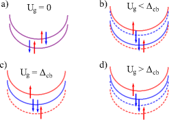
Figure 4: Schematic evolution of the four low-energy CB bands as a function of the inter-layer potential $U_{g}$ at the $K$ point of the BZ. Spin-degenerate bands are shown with purple, $\uparrow$ polarized with red and $\downarrow$ polarized with blue. Solid line corresponds to bands at $+U_{g}$, dashed line to bands at $-U_{g}$ potential.

We note that in recent experimentsvalley-Hall-BLMoS2 ; Morpurgo-3R-bilayer the bilayer devices were fabricated with a single backgate. In such devices the bilayer would be doped and at the same time a finite inter-layer potential difference $U_{g}$ would be induced by changing the backgate voltage. Depending on the $E_{F}/U_{g}$ and $E_{F}/\Delta_{cb}$ ratios, where $E_{F}$ is the Fermi energy, only one or both layers [this case is illustrated in Fig. 2(d)] and $1-4$ bands may contribute to $\sigma_{v,H}^{2H}$ and $\sigma_{s,H}^{2H}$. In the following we will assume that $E_{F}>2(U_{g}+\Delta_{cb})$ for all $U_{g}$ values considered, i.e., $E_{F}$ is large enough so that both layers and all four low-energy CBs are occupied and contribute to the valley and spin Hall effects. In MoS₂, given the relatively small $\Delta_{cb}\approx 3$meV value of the SOC, we expect that this situation is realistic. However, in other 2H-BTMDCs where the SOC constant $\Delta_{cb}$ can be substantially larger than in MoS₂, not all four CBs would be necessarily occupied. Furthermore, we neglect any Rashba type SOC induced by the external electric field because we expect that in the devices of Refs. valley-Hall-BLMoS2, ; Morpurgo-3R-bilayer, it should be much smaller than the intrinsic SOC. We also neglect the difference between the effective masses of the two spin-split CBs at $U_{g}=0$ because it is quite small in MoS₂ and use a single effective mass $m_{\rm eff}$ for all bands. On the other hand, as shown in Fig. 2(b), for $U_{g}\lesssim 20$meV the $\mathbf{q}$ dependence of $\Omega_{z,cb}(\mathbf{q})$ is more important for 2H bilayers than for 3R bilayers and we take it into account when we evaluate Eqs. (8) and (9).

We first assume that $U_{g}\lessgtr\Delta_{cb}$ and that $E_{F}\sim$ few tens of  meV. The case $U_{g}=\Delta_{cb}$, which requires slightly different considerations, will be discussed below (see also Appendix D). Under the above assumptions and after summing up the contributions of all four bands shown in Fig. 4, one finds that

$$\sigma_{v,H}^{2H}\approx\tau\frac{e^{2}}{\hbar}\left[\frac{\varepsilon_{cc}}{2\pi}\frac{U_{g}}{U_{g}^{2}-\Delta_{cb}^{2}}-\rho_{2d}U_{g}\left(\frac{\gamma_{3}}{\delta E_{bg}}\right)^{2}\lambda_{4}(U_{g})\right],$$ (12)

and

$$\sigma_{s,H}^{2H}\approx-\left[\frac{\varepsilon_{cc}}{2\pi}\frac{\Delta_{cb}}{U_{g}^{2}-\Delta_{cb}^{2}}+\rho_{2d}\Delta_{cb}\left(\frac{\gamma_{3}}{\delta E_{bg}}\right)^{2}\lambda_{4}(U_{g}).\right]$$ (13)

Here $\varepsilon_{cc}=\frac{2m_{\rm eff}}{\hbar^{2}}\gamma_{cc}^{2}$, $\rho_{2d}=m_{\rm eff}/2\pi\hbar^{2}$ is the two-dimensional density of states per spin and valley, and $\lambda_{4}(U_{g})=\left(1+\frac{3}{4}\frac{\Delta_{vb}^{2}+t_{\perp}^{2}+U_{g}^{2}}{\delta E_{bg}^{2}}\right)$. One can see that $\sigma_{v,H}^{2H}$ vanishes for $U_{g}\rightarrow 0$, but $\sigma_{s,H}^{2H}$ remains finite. When $U_{g}$ is of the order of $\Delta_{cb}$, the first term on the r.h.s of Eqs. (12) and (13), which is related to the inter-layer contribution to the Berry curvature, is larger than the second term. Moreover, this term changes sign as $U_{g}$ is changed from $U_{g}<\Delta_{cb}$ to $U_{g}>\Delta_{cb}$ and we expect that this leads to a sign change in $\sigma_{v,H}^{2H}$ and $\sigma_{s,H}^{2H}$. It is interesting to note that in e.g., lattice Chern insulators such a sign change of the off-diagonal conductivity was associated with a topological transition. In our case the sign change of $\sigma_{v,H}^{2H}$ and $\sigma_{s,H}^{2H}$ happens as the $\downarrow$ ($\uparrow$) bands first become degenerate at the $K$ ($-K$) point and then the degeneracy is lifted again as the electric field is increased further.

Regarding the $U_{g}=\Delta_{cb}$ case when two spin-polarized bands become degenerate [see Fig.4(c)], in good approximation only the bands that remain non-degenerate have finite valley and spin Hall conductivity (see Appendix D). Therefore the magnitude of $\sigma_{v,H}^{2H}$ and $\sigma_{s,H}^{2H}$ is the same (apart from the fact that they are measured in different units). Summing up the contributions of the two $\uparrow$ ($\downarrow$) bands in the $K$ ($-K$) valleys, one finds that $\sigma_{v,H}^{2H}\approx\tau\frac{e^{2}}{\hbar}\tilde{\sigma}_{v,H}$ and $\sigma_{s,H}^{2H}\approx\tilde{\sigma}_{v,H}$, where

$$\tilde{\sigma}_{v,H}\approx\frac{1}{2}\left(\frac{\varepsilon_{cc}}{4\pi\Delta_{cb}}-\rho_{2d}\Delta_{cb}\left(\frac{\gamma_{3}}{\delta E_{bg}}\right)^{2}\lambda_{5}\right)$$ (14)

and $\lambda_{5}=\left(1+\frac{3}{4}\frac{(\Delta_{vb})^{2}+t_{\perp}^{2}}{\delta E_{bg}^{2}}\right)$.

We do not discuss here the case when not all four spin-split bands below the $E_{F}$ are occupied because we expect that relatively large doping levels may be needed to suppress many-body effects, which are beyond the scope of the present work.

VI The $Q$ valleys

As one can see in, e.g., Figs. 1(a) and 1(b), the local minimum of the CB at the $Q$ point of the BZ is almost degenerate with the $K$ valley, especially for 2H stacking. In our DFT band structure calculations the band edge is at the $K$ point for both stackings and the $Q$ valleys would only be populated for a relatively strong $n$-doping. We show the calculated $\delta E_{QK}$ values, i.e., the energy difference between the bottom of the $Q$ and the $K$ valleys, without/with taking into account SOC, in Table 2 below.

	noSOC	SOC
2H	$9$ meV	$10$ meV
3R	$75$ meV	$51$ meV

Table 2: The calculated $\delta E_{QK}$ values for 2H and 3R bilayers without (no SOC) and with (SOC) taking into account the SOC.

We note that in the case of monolayers it was found that $\delta E_{QK}$ depends quite sensitively on the lattice constant, exchange-correlation potential2DMaterials-paper and it may also depend on the level of theory (DFT or GW) used in the calculations. The same is expected to be the case for bilayers as well, where in addition the inter-layer separation used in the calculations may also influence the location of the band edge.

Irrespective of the exact value of $\delta E_{QK}$ in DFT calculations, it is of interest to understand if the six $Q$ valleys can affect the valley Hall conductivity described in Section V because strain or interaction with a substrate may also affect energy difference between the bottom of the $K$ and $Q$ valleys. The calculations of Ref. JinboYang, indicate that the Berry curvature is very small at the $Q$ point of monolayer TMDCs, therefore in our case it is only the inter-layer contribution that needs to be considered. We find that, generally, the Berry curvature should be significantly smaller in the $Q$ valley than in the $K$ valley for bilayer MoS₂ (see Appendix C). This is mainly because the bands are split by a momentum independent tunnelling amplitude $t_{\perp,Q}$ which is much larger than the energy scale for momentum dependent coupling and the intra-layer spin-splitting. Therefore, as long as inter-valley scattering between the $K$ and $Q$ valleys is not strong, the $Q$ valleys should have only a minor effect on the valley Hall and spin Hall conductivities. Moreover, since the intra-layer spin-orbit coupling $\Delta_{Q}$ is one order of magnitude larger than $\Delta_{cb}$ at the $K$ point, we do not expect that in double gated devices a topological transition similar to the one at the $K$ point can take place.

VII Discussion and summary

In a very recent workKTLaw-spinHall a different type of electrically controllable valley Hall effect, due to the Rashba type SOC, was proposed in gated monolayer TMDCs. In order to obtain appreciable Rashba SOC in monolayer MoS₂, one would need rather strong displacement fieldsPRX-paper of the order of $0.3-0.4$ eVÅQun-Fang , which are attainable, e.g., in ionic liquid gated devices. In contrast, given an inter-layer distance of $d=2.975$Å,  a displacement field of $0.04$ eVÅ  would lead to an inter-layer potential difference $U_{g}\approx 13\,$meV which would give a roughly two-fold increase of $\Omega_{z,cb}$ in 2H bilayers with respect to the monolayer value. Thus we think that the Berry curvature is more easily tunable in bilayer TMDCs than in monolayers.

Another way of investigating the Berry curvature may be offered by optical methods, where one can make use of the selection rules for circularly polarized light for intra-layer excitonic transitions at the $\pm K$ point. As it was shown in Refs. Srivastava, ; JZhou, for monolayer TMDCs, the Berry curvature acts as a momentum-space magnetic field and therefore it can split the energies of excitons that have non-zero angular momentum number. By extending this argument to bilayers, one may expect that the Berry curvature should lead to a splitting of intra-layer excited excitonic states with non-zero angular momentum number and the effect would be more pronounced, especially in 2H bilayers, than in monolayers. Note, that the Berry curvature of both the CB and the VB would contribute to this effectSrivastava ; JZhou . This would constitute a novel mechanism to influence intra-layer excitonic properties: the other layer does not only provide screening, but acts through the changing of the Berry curvature of the electrons and holes.

In summary, we have studied the Berry curvature properties and the corresponding valley Hall conductivities of bilayer MoS₂. We have considered both 3R and 2H stacked bilayers and found intra-layer as well as inter-layer contributions to the Berry curvature, a situation not discussed before for layered materials. Due to the inter-layer contribution, the Berry curvature is gate tunable. Moreover, we found that in 3R stacked bilayers the Berry curvature is much larger for electronic states in one of the layers than in the other one, i.e., it is effectively localized to one of the layers. For 2H stacking, on the other hand, it is usually much larger in the CB than in the VB, but it has the same magnitude in both layers. We studied the consequences of the Berry curvature for n-doped samples. Firstly, the valley Hall conductivity will be finite if inversion symmetry is broken. Secondly, if the intrinsic SOC of the constituent layers is taken into account, the spin Hall conductivity is finite. Due to the SOC, in 3R bilayers all bands are non-degenerate and spin-polarized, while in 2H bilayers the spin-polarized bands of the monolayer constituents are energetically degenerate as long as inversion symmetry is not broken. In 2H bilayers the interplay of SOC and finite interlayer potential can lead to a topological transition for one pair of spin-polarized bands. This leads to a change in the sign of the inter-layer contribution to the valley and spin Hall effects, while the intra-layer contribution does not change sign. Our work highlights the role of the stacking, intra- and interlayer couplings on certain topological properties and can be relevant to a wide range of van der Waals materials.

VIII Acknowledgement

A. K. and G. B. acknowledge funding from FLAG-ERA through project “iSpinText” and from SFB767. V. Z. and V. F. acknowledge support from the European Graphene Flagship Project, the N8 Polaris service, and the use of the ARCHER supercomputer (RAP Project e547).

Appendix A Derivation of $\mathbf{k}\cdot\mathbf{p}$ Hamiltonians of bilayer TMDCs

We remind that the symmetry properties of a band $\eta$ at a given $\mathbf{k}$-space point can be deduced by considering the transformation properties of Bloch states of the form PRB-paper

$$| \Psi_{\eta}^{t(b)}(\mathbf{k},\mathbf{r})\rangle\equiv|\Psi_{l,m}^{t(b)}(\mathbf{k},\mathbf{r})\rangle$$ (15)

$$= \frac{1}{\sqrt{N}}\sum_{\mathbf{R}_{n}}e^{i\mathbf{k}(\mathbf{R}_{n}+\mathbf{t}_{Mo}^{t(b)})}Y_{l}^{m}(\mathbf{r}-[\mathbf{R}_{n}+\mathbf{t}_{Mo}^{t(b)})],$$

where $Y_{l}^{m}(\mathbf{r})$ are rotating orbitals formed from the atomic orbitals that contribute with large weight to a given band $\eta$ at a given $\mathbf{k}$-space point, $\mathbf{R}_{n}$ are lattice vectors in the direct lattice and $\mathbf{t}_{Mo}^{t(b)}$ give the positions of the Mo atoms in the top ($t$) and bottom ($b$) layers in the 2D unit cell. In the case of 2H bilayers in external electric field the label $t$ corresponds to the layer at $+U_{g}$ potential, while the label $b$ to the layer at $-U_{g}$ potential. For zero electric field the labels $t$ and $b$ are somewhat arbitrary, nevertheless, for convenience we will keep them in the discussion that follows. (More rigorously, if the geometric position of the three-fold rotation axis is fixed, then each band can be labelled by an irreducible representation of the pertinent group of the wave vector. Our choice of the lattice vectors and the coordinate system is shown below in Figure 5.) The situation is different for 3R bilayers: as explained in the main text, here the two layers are not equivalent and one can define unambiguously the layer indices $t$ and $b$.

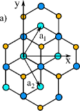
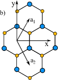
Figure 5: Schematic top view of the crystal lattice of a) 3R and b) 2H bilayer TMDC. For 3R bilayers in a) the position of the metal atoms in the unit cell are given by the vectors $\mathbf{t}_{Mo}^{t}=\frac{a}{2}(1,-1/\sqrt{3})^{T}$ and $\mathbf{t}_{Mo}^{b}=(0,0)^{T}$. Metal atoms in different layers are shown by different colours. For 2H bilayers in b) only atoms in the top layer are visible. The position of the metal atoms in the unit cell are given by the vectors $\mathbf{t}_{Mo}^{t}=\frac{a}{2}(1,-1/\sqrt{3})^{T}$ and $\mathbf{t}_{Mo}^{b}=\frac{a}{2}(1,1/\sqrt{3})^{T}$. Here $a$ is the lattice constant.

The $\mathbf{k}\cdot\mathbf{p}$ Hamiltonian at a given $\mathbf{k}$-space point (see Fig. 6 for the Brillouin zone) can be then found by considering the transformation properties of the matrix elements $\langle\Psi_{\eta}^{\nu}(\mathbf{k},\mathbf{r})|\mathbf{\hat{p}}|\Psi_{\eta^{\prime}}^{\nu^{\prime}}(\mathbf{k},\mathbf{r})\rangle$, where $\nu,\nu^{\prime}=\{t,b\}$ and $\mathbf{\hat{p}}=(\hat{p}_{x},\hat{p}_{y})$ are momentum operators (for details see, e.g., Refs. PRB-paper, ; 2DMaterials-paper, ). In this way one can arrive at a $7\times 7$ model of a monolayer TMDCs2DMaterials-paper and a corresponding $14\times 14$ model for bilayers. Similarly, the SOC matrix elements can be found by considering $\langle\Psi_{\eta}^{\nu}(\mathbf{k},\mathbf{r})|\mathbf{\hat{L}}\cdot\mathbf{\hat{S}}|\Psi_{\eta^{\prime}}^{\nu^{\prime}}(\mathbf{k},\mathbf{r})\rangle$ where $\mathbf{\hat{L}}$ is a vector of angular momentum operators and $\mathbf{\hat{S}}$ is a vector of spin operators. In some cases, especially for effective Hamiltonians, it is easier to use the theory of invariantsBirPikus . Both approaches lead to the same results. We will use the following notation. The Pauli matrices $\sigma_{x,y,z}$ act in the space of top ($t$) and bottom ($b$) layer, while the Pauli matrices $s_{x,y,z}$ act in the space of the spin degree of freedom. $\uparrow$ and $\downarrow$ denote the eigenstates of $s_{z}$. Finally, the Pauli matrix $\tau_{z}$ describes the valley degree of freedom, and whenever convenient, we use its eigenvalues $\tau=\pm 1$ for the same purpose.

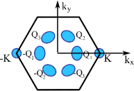
Figure 6: The Brillouin zone with the six $Q$ points and the $\pm K$ valleys.

Appendix B $\mathbf{k}\cdot\mathbf{p}$ Hamiltonians at the $\pm K$ point of the Brillouin zone

B.1 2H bilayer

B.1.1 $\mathbf{k}\cdot\mathbf{p}$ Hamiltonian

In the discussions below we will refer to the group of the wavevector at the $\mathbf{k}=\pm K=\pm\frac{4\pi}{3a}(1,0)^{T}$ points of the BZ, which is ${D}_{3}$ for this stacking ($a$ is the length of the lattice vectors $\mathbf{a}_{1}$, and $\mathbf{a}_{2}$). The character table of ${D}_{3}$ is given below in Table 3.

	E	$2C_{3}$	$3C_{2}$
$\Gamma_{1}$	1	1	1
$\Gamma_{2}$	1	1	-1
$\Gamma_{3}$	2	-1	0

Table 3: Character table of the point group ${D}_{3}$.

We remind that in monolayer TMDCs the atomic $d_{z^{2}}$ orbitals of the metal atoms contribute with largest weight to the CB at the $\pm K$ points of the BZ. Regarding the VB, the $d_{xy}$ and $d_{x^{2}-y^{2}}$ orbitals are important at the $\pm K$ points. Taking into account that in 2H bilayers one of the monolayers is rotated by $180^{\circ}$ with respect to the otherWangYao-bilayer , one finds that the minimal basis set to describe the CB are the Bloch wavefunctions $|\Psi_{2,0}^{t(b)}(K,\mathbf{r})\rangle$ and for the VB the $|\Psi_{2,-2}^{t}(K,\mathbf{r})\rangle$, $|\Psi_{2,2}^{b}(K,\mathbf{r})\rangle$ (This means that the top layer “inherits” the convention we used in Refs. PRB-paper, ; 2DMaterials-paper, for monolayer TMDCs, which is that at the $K$ point the Bloch wavefunction of the valence band is $|\Psi_{2,-2}(K,\mathbf{r})\rangle$).

As a first step, let us neglect the SOC. Using the coordinate system shown in Figure 5(b), one can easily show that $|\Psi_{2,0}^{t}(K,\mathbf{r})\rangle$ and $|\Psi_{2,0}^{b}(K,\mathbf{r})\rangle$ transform as partners of the two-dimensional irreducible representation (irrep) $\Gamma_{3}$ of ${D}_{3}$. This means that the CB is doubly degenerate at the $K$ point. We have checked that in our DFT calculations this is indeed the case (within numerical accuracy). Regarding the VBs, $|\Psi_{2,-2}^{t}(K,\mathbf{r})\rangle$ transforms as one of the partners of the irrep $\Gamma_{3}$, while $|\Psi_{2,2}^{b}(K,\mathbf{r})\rangle$ transforms as irrep $\Gamma_{1}$. Since the Bloch wavefunctions of the VBs of the $t$ and $b$ layers transform according to different irreps, the VB of the bilayer is not degenerate. One can also notice that the operators $\hat{p}_{\pm}=\hat{p}_{x}\pm i\hat{p}_{y}$ also transform as partners of the irrep $\Gamma_{3}$. Using the basis $\{|\Psi_{\rm cb}^{t}\rangle,|\Psi_{\rm vb}^{t}\rangle,|\Psi_{\rm cb}^{b}\rangle,|\Psi_{\rm vb}^{b}\rangle\}$, the above considerations then lead to the following $\mathbf{k}\cdot\mathbf{p}$ Hamiltonian:

$$H^{2H}_{K}=\left(\begin{array}[]{cccc}\varepsilon_{cb}&\gamma_{3}\,q_{+}&\gamma_{cc}\,q_{-}&\gamma_{cv}q_{+}\\ \gamma_{3}\,q_{-}&\varepsilon_{vb}&\gamma_{vc}q_{+}&t_{\perp}\\ \gamma_{cc}\,q_{+}&\gamma_{vc}q_{-}&\varepsilon_{cb}&\gamma_{3}q_{-}\\ \gamma_{cv}q_{-}&t_{\perp}&\gamma_{3}q_{+}&\varepsilon_{vb}\end{array}\right).$$ (16)

Here $t_{\perp}$ is a momentum independent tunneling amplitude between the VBs, $\gamma_{3}$ is the intra-layer coupling between the VB and the CB in each layer, while $\gamma_{cc}$ and $\gamma_{vc}=\gamma_{cv}$ are inter-layer couplings. Here $q_{\pm}=\tau q_{x}\pm iq_{y}$ denotes the wavenumber measured from the $K$ (or $-K$) point of the BZ and $\tau=\pm 1$ is the valley index. A similar Hamiltonian to (16), which only considered $t_{\perp}$ and neglected all other inter-layer coupling, was derived in Ref. WangYao-bilayer . We found that close to the $K$ point the dispersion of the CB and VB obtained from DFT calculations can be fitted quite well by assuming that the inter-layer inter-band coupling constant $\gamma_{cv}$ is small and therefore we neglected this term. In contrast, the term $\sim\gamma_{cc}$ is needed both to accurately fit the DFT band structure and for the Berry curvature calculations.

B.1.2 Spin-orbit coupling

For simplicity, we will only discuss here the case of zero external electric field. Time reversal and inversion symmetries dictate that all bands are spin-degenerate throughout the BZ. In the simplest approximation we may take into account only the SOC in the constituent monolayers. Using the basis $|\{\Psi_{\rm cb}^{t}\uparrow\rangle,|\Psi_{\rm cb}^{t}\downarrow\rangle,|\Psi_{cb}^{b}\uparrow\rangle,|\Psi_{cb}^{b}\downarrow\rangle\}$ for the CB (and an analogous basis set for the VB), the SOC Hamiltonian is

$$H_{\rm cb(vb),SOC}^{(1)}=\Delta_{cb(vb)}\tau_{z}\sigma_{z}s_{z}$$ (17)

Our DFT calculations show that the monolayer values $\Delta_{cb}$ and $\Delta_{vb}$ are indeed very close to the values $\Delta_{cb}^{bl}$, $\Delta_{vb}^{bl}$ found in bilayers. The term in Eqs. (17) is the most important one close to the $\pm K$ points.

Strictly speaking, however, $H_{\rm cb(vb),SOC}^{(1)}$ is not the only SOC term allowed by symmetries. Further terms can be obtained by using an extended $\mathbf{k}\cdot\mathbf{p}$ model for the monolayers as in Ref. 2DMaterials-paper, . For bilayers this extended basis contains $28$ basis states. The resulting SOC Hamiltonian has matrix elements that connect basis states within the same layer as well as inter-layer matrix elements. To simplify the discussion, we project the SOC onto the CBs and the VBs closest to the band gap. Then one can also use the theory of invariants to derive the SOC terms that appear in this effective low-energy model. For example, as already mentioned, the basis states $|\Psi_{2,0}^{t}(K,\mathbf{r})\rangle$ and $|\Psi_{2,0}^{b}(K,\mathbf{r})\rangle$ transform as partners of the two-dimensional irreducible representation $\Gamma_{3}$ of ${D}_{3}$. This means that for the CB one can adapt the results derived for bilayer grapheneWinkler-BLG ; JFabian-bilayer ; trilayer-SOC and siliceneTrauzettel-silicene , where the low-energy sector of the Hamiltonian is also spanned by basis vectors transforming according to irrep $\Gamma_{3}$ of $D_{3}$. One finds that in lowest order of $\mathbf{k}$, in addition to the Eq. (17), one more term is allowed:

$$H_{cb,SOC}^{(2)}=\Delta_{cb(vb)}^{(2)}\sigma_{z}(s_{x}q_{y}-s_{y}q_{x}).$$ (18)

Similarly to the CB, one finds that a term

$$H_{vb,SOC}^{(2)}=\Delta_{vb}^{(2)}\sigma_{z}(s_{x}q_{y}-s_{y}q_{x})$$ (19)

can be added to the low-energy Hamiltonian in the VB. As one can see $H_{cb(vb),SOC}^{(2)}$ introduces a Rashba-like coupling within each of the layers.

We note that although $H_{cb(vb),SOC}^{(2)}$ is diagonal in the layer space, a similar term is absent in monolayers. This follows from the different symmetries of monolayers and bilayers. In monolayer TMDCs the pertinent symmetry group at $\pm K$ points is the $C_{3h}$ point group. This point group contains the symmetry element $\sigma_{h}$ corresponding to a horizontal mirror plane. Polar vectors (such as $q_{x}$, $q_{y}$) and axial vectors (such as $s_{x}$, $s_{y}$) transform differently under $\sigma_{h}$ and therefore terms that contain their products, such as those in Eq. (18), are not allowed. In the case of bilayer TMDCs the pertinent point group for the wavevector is $D_{3}$, which does not discriminate between polar and axial vectors and hence terms containing the products of wavenumber and spin components become admissible.

From a more microscopic point of view one can show that $H_{cb,SOC}^{(2)}$ and $H_{vb,SOC}^{(2)}$ are both due to an interplay of i) wavenumber dependent intra-layer coupling to higher or lower energy orbitals, and ii) certain off-diagonal intra-layer SOC matrix elements. The details of these calculations will be given elsewhere. The coupling constant $\Delta_{cb}^{(2)}$ and $\Delta_{vb}^{(2)}$ appear to be small in MoS₂ and we could not reliably extract them from our DFT calculations.

B.2 3R bilayer

B.2.1 $\mathbf{k}\cdot\mathbf{p}$ Hamiltonian

The 3R bilayer has lower symmetry than 2H bilayers, e.g., as already mentioned in the main text, the crystal structure lacks inversion symmetry. The group of the wavevector at the $\pm K$ points of the BZ is $C_{3}$, for the character table see Table 4.

	E	$C_{3}$	$C_{3}^{2}$
$\Gamma_{1}$	1	1	1
$\Gamma_{2}$	1	$\omega$	$\omega^{2}$
$\Gamma_{3}$	1	$\omega^{2}$	$\omega$

Table 4: Character table of the group ${C}_{3}$. Here $\omega=e^{2i\pi/3}$.

One can see that all irreps of $C_{3}$ are one-dimensional. This suggest that the bands of 3R bilayers are non-degenerate in the $\pm K$ valleys.

Using the coordinate system shown in Figure 5(a), the basis state $|\Psi_{2,0}^{t}(K,\mathbf{r})\rangle$ ($|\Psi_{2,0}^{b}(K,\mathbf{r})\rangle$) in the CB of the top (bottom) layer transforms as $\Gamma_{2}$ ($\Gamma_{1}$) of $C_{3}$. Regarding the VB, one finds that $|\Psi_{2,-2}^{t}(K,\mathbf{r})\rangle$ ($|\Psi_{2,-2}^{b}(K,\mathbf{r})\rangle$) transforms as $\Gamma_{1}$ ($\Gamma_{3}$). In the basis $\{|\Psi_{\rm cb}^{b}\rangle,|\Psi_{\rm vb}^{b}\rangle,|\Psi_{\rm cb}^{t}\rangle,|\Psi_{\rm vb}^{t}\rangle\}$ these symmetry considerations then lead to the following general form of the $\mathbf{k}\cdot\mathbf{p}$ Hamiltonian

$$H^{3R}_{K}=\left(\begin{array}[]{cccc}\varepsilon_{cb}^{b}&\gamma_{3}\,q_{+}&\gamma_{cc}\,q_{-}&t_{cv}\\ \gamma_{3}\,q_{-}&\varepsilon_{vb}^{b}&\gamma_{vc}q_{+}&\gamma_{vv}\,q_{-}\\ \gamma_{cc}\,q_{+}&\gamma_{vc}q_{-}&\varepsilon_{cb}^{t}&\gamma_{3}q_{+}\\ t_{cv}&\gamma_{vv}q_{+}&\gamma_{3}q_{-}&\varepsilon_{vb}^{t}\end{array}\right).$$ (20)

Here we assumed that the diagonal elements $\varepsilon^{t}$ and $\varepsilon^{b}$ can be different in the two layers. This can be motivated by noticing that the Mo atoms in the two layers have different chemical environment, since one of them is above a sulphur atom of the other layer, while the second Mo atom can be found in a hollow position. In contrast, in the crystal structure of 2H bilayers the metal atoms in the two layers have the same chemical environment and therefore one expects that the diagonal elements of the effective Hamiltonians are the same in the two layers, see Eq. (16). This argument can also be formulated from a symmetry point of view: in 2H bilayers the metal atoms are connected by symmetry operations of the crystal lattice, while this is not the case in 3R bilayers.

Looking at Eq. (20), one can notice that the tunnelling amplitude $t_{cv}$, in principle, introduces a band repulsion between the CB of the bottom layer and the VB of the top layer even for $\mathbf{q}=0$. This looks similar to the situation in 2H bilayers, where such a tunnelling element appears between the two VB states, see Eq. (16). Indeed, in a recent workXiaoou on the selection rules of optical transitions in 3R bilayers an estimate of $t_{cv}\approx 50$ meV was given, which is comparable to $t_{\perp}$ in 2H bilayers. However, the analysis of our DFT calculations suggests that $t_{cv}$ in 3R bilayers is much smaller than $t_{\perp}$. To substantiate this claim we show firstly the weight of the atomic orbitals in the highest energy VB of 2H bilayers at the $K$ point, as obtained from DFT calculations, in Table 5. Only atomic orbitals with non-zero weight are included.

	$p_{y}$	$p_{x}$	$d_{xy}$	$d_{x^{2}-y^{2}}$	tot
Mo(b)	$0.0$	$0.0$	$0.166$	$0.166$	$0.333$
Mo(t)	$0.0$	$0.0$	$0.167$	$0.167$	$0.334$
S${}^{(b)}_{1}$	$0.017$	$0.017$	$0.0$	$0.0$	$0.034$
S${}^{(b)}_{2}$	$0.017$	$0.017$	$0.0$	$0.0$	$0.034$
S${}^{(t)}_{1}$	$0.017$	$0.017$	$0.0$	$0.0$	$0.034$
S${}^{(t)}_{2}$	$0.017$	$0.017$	$0.0$	$0.0$	$0.034$

Table 5: The weight of the atomic orbitals in the highest valence band of 2H bilayer MoS₂ at the $K$ point of the BZ. Mo^(b) (Mo^(t)) stands for the molybdenum atom in the top (bottom) layer. Similarly, S${}^{(b)}_{1}$ and S${}^{(b)}_{2}$ (S${}^{(t)}_{1}$ and S${}^{(t)}_{2}$) stands for the two sulphur atoms in the two layers.

As one can see, the atomic orbitals of both layers contribute with equal weight to this band. This agrees with the conclusion that one could draw from the Hamiltonian (2): by diagonalizing it at $\mathbf{q}=0$, one can see that the VB states of the two layers form “bonding” and “antibonding” states due to the tunnelling $t_{\perp}$. In these new states the weight of the states from each layer is the same. Moreover, we find the same atomic weights as shown in Table 5 for the second highest energy VB, which again supports the above interpretation.

In the case of 3R bilayers, a similar argument would suggest that both atomic orbitals belonging to the bottom layer and orbitals belonging to the top layers would have finite weight in one of the CBs. In Tables 6 and 7 we show the weight of the atomic orbitals in the first and second CB of 3R bilayer MoS₂, respectively. The SOC is neglected in these calculations since it is not important for the argument that we make.

	$s$	$p_{x}$	$p_{y}$	$d_{z^{2}}$
Mo(b)	$0.0$	$0.0$	$0.0$	$0.0$
Mo(t)	$0.043$	$0.0$	$0.0$	$0.743$
S${}^{(b)}_{1}$	$0.0$	$0.0$	$0.0$	$0.0$
S${}^{(b)}_{2}$	$0.0$	$0.0$	$0.0$	$0.0$
S${}^{(t)}_{1}$	$0.0$	$0.017$	$0.017$	$0.0$
S${}^{(t)}_{2}$	$0.0$	$0.017$	$0.017$	$0.0$

Table 6: The weight of the atomic orbitals in the first conduction band of 3R bilayer MoS₂ at the $K$ point of the BZ. Mo^(b) (Mo^(t)) stands for the molybdenum atom in the top (bottom) layer. Similarly, S${}^{(b)}_{1}$ and S${}^{(b)}_{2}$ (S${}^{(t)}_{1}$ and S${}^{(t)}_{2}$) stands for the two sulphur atoms in the top (bottom) layer.

	$s$	$p_{x}$	$p_{y}$	$d_{z^{2}}$
Mo(b)	$0.043$	$0.0$	$0.0$	$0.744$
Mo(t)	$0.0$	$0.0$	$0.0$	$0.0$
S${}^{(b)}_{1}$	$0.0$	$0.016$	$0.016$	$0.0$
S${}^{(b)}_{2}$	$0.0$	$0.017$	$0.017$	$0.0$
S${}^{(t)}_{1}$	$0.0$	$0.0$	$0.0$	$0.0$
S${}^{(t)}_{2}$	$0.0$	$0.0$	$0.0$	$0.0$

Table 7: The same as in Table 6 but for the second conduction band of 3R bilayer MoS₂ at the $K$ point of the BZ.

According to our DFT calculations the atomic orbitals from the two layers are not admixed, i.e., the two layers are practically decoupled at the $K$ point. The results in Table 6 and 7 therefore suggest that $t_{cv}$, although allowed to be non-zero by symmetry considerations, is probably very small. We think that the splitting of both the VB and CB states that can be clearly seen in Figure 1(a) of the main text is due to the difference between the band edge energies $\varepsilon_{cb}^{b}$ and $\varepsilon_{cb}^{t}$ ($\varepsilon_{vb}^{b}$ and $\varepsilon_{vb}^{t}$). This is the reason why we neglected $t_{cv}$ in the effective $\mathbf{k}\cdot\mathbf{p}$ model used in the main text.

B.2.2 Spin-orbit coupling

Since inversion symmetry is broken by the lattice in 3R bilayers, the bands need not be spin-degenerate when SOC is taken into account. We will use the basis $\{|\{\Psi_{\rm cb}^{b}\uparrow\rangle,|\Psi_{\rm cb}^{b}\downarrow\rangle,|\Psi_{cb}^{t}\uparrow\rangle,|\Psi_{cb}^{t}\downarrow\rangle\}$ and an analogous basis for the VB. Considering only the SOC coupling of the constituent monolayers, the SOC Hamiltonians are

$$H_{cb(vb),SOC}^{(1)}=\Delta_{cb(vb)}\tau_{z}s_{z},$$ (21)

for the CB and the VB, respectively. Note that, in contrast to the 2H bilayers [see Eq. (17)] the Hamiltonian (21) does not depend on $\sigma_{z}$, i.e., it is independent of the layer index. This is in agreement with the findings of Ref. Arita, . $H_{cb(vb),SOC}^{(1)}$ leads to the splitting of the otherwise spin degenerate CB and VB in each of the layers. These bands are therefore non-degenerate and the spin-polarization of the bands is the same in both layers.

Similarly to the 2H case, further SOC terms become possible if one considers virtual intra-layer and inter-layer processes. To simplify the discussion, we project the SOC onto the CBs and the VBs closest to the band gap. We list here the possible terms for the CBs, the same terms, albeit with different SOC strength, can be obtained for the VBs. Firstly, the intra-layer processes give rise to a term similar to Eq. (18):

$$H_{cb,so}^{(2,t(b))}=\Delta_{cb}^{(2,t(b))}(s_{x}q_{y}-s_{y}q_{x}),$$ (22)

where in general the SOC coupling strengths are different in the two layers: $\Delta_{cb}^{(2,b)}\neq\Delta_{cb}^{(2,t)}$. Due to the lower symmetry of the 3R stacking, one finds further three non-zero inter-layer SOC terms. Defining $\sigma_{\pm}=(\sigma_{x}\pm i\sigma_{y})/2$ and $s_{\pm}^{\tau}=(s_{x}\pm i\tau s_{y})/2$, one may write the first one as

$$H_{cb,so}^{(3)}=i\Delta_{cb}^{(3)}(\sigma_{+}s_{-}^{\tau}-\sigma_{-}s_{+}^{\tau})=\frac{\Delta_{cb}^{(3)}}{2}(\tau_{z}\sigma_{x}s_{y}-\sigma_{y}s_{x})$$ (23)

where $\Delta_{cb}^{(3)}$ describes direct spin-flip tunnelling between the CBs of the two layers. The second one reads

$$H_{cb,so}^{(4)} =i\tau\Delta_{cb}^{(4)}(\sigma_{+}s_{+}^{\tau}q_{+}^{\tau}-\sigma_{-}s_{-}^{\tau}q_{-}^{\tau})$$

$$= -\frac{\Delta_{cb}^{(4)}}{2}[\sigma_{x}(s_{x}q_{y}+s_{y}q_{x})+\tau_{z}\sigma_{y}(s_{x}q_{x}-s_{y}q_{y})],$$

and the third one is

$$H_{cb,so}^{(5)}=\Delta_{cb}^{(5)}[\sigma_{+}q_{-}^{\tau}+\sigma_{-}q_{+}^{\tau}]s_{z}=\Delta_{cb}^{(5)}[\sigma_{x}q_{x}+\tau_{z}\sigma_{y}q_{y}]s_{z}.$$ (25)

One can show that the last two terms, $H_{cb,so}^{(4)}$ and $H_{cb,so}^{(5)}$ are due to the interplay of a spin-dependent intra-layer hopping to a higher or lower energy orbital followed by a spin-independent inter-layer tunnelling or vice versa, a spin-independent intra-layer hopping followed by a spin-dependent inter-layer tunnelling.

Our DFT calculations suggest that in MoS₂ the terms corresponding to Eqs. (22)-(25) are much smaller than the monolayer SOC term Eq. (21). Moreover, we find that $\delta E_{cc}=(\varepsilon_{cb}^{b}-\varepsilon_{cb}^{t})/2\gg\Delta_{cb}^{(1)}$, which means that the low-energy CB bands are localized to the top layer. In contrast, $\delta E_{vv}=(\varepsilon_{vb}^{b}-\varepsilon_{vb}^{t})/2$ and $\Delta_{vb}^{(1)}$ are of similar magnitude in MoS₂ and following the convention of Ref. 2DMaterials-paper, , whereby $\Delta_{vb}<0$ at the $K$ point, the highest energy state at $K$ is $|\Psi_{\rm vb}^{b}\downarrow\rangle$, followed by $|\Psi_{vb}^{t}\downarrow\rangle$, $|\Psi_{\rm vb}^{b}\uparrow\rangle,$ and finally $|\Psi_{vb}^{t}\uparrow\rangle$.

Looking beyond MoS₂, in other MX₂ bilayers it may happen that the crystal field splitting $\delta E_{cc}$ and the SOC strength $\Delta_{cb}^{(1)}$ are of comparable magnitude. In this case the two lowest energy CB bands would be localized on different layers, in the same way as in the VB of bilayer MoS₂.

Appendix C $\mathbf{k}\cdot\mathbf{p}$ Hamiltonians at the $Q$ points of the Brillouin zone

In addition to the valleys at the $\pm K$ points, there are six $Q$ valleys in the CB, see Fig. 6. Although in our DFT calculations the band edge in the CB can always be found at the $\pm K$ point, the minima at the $Q$ points is close in energy to the minima at the $\pm K$ point [see Section VI in themain text]. For finite doping therefore it may happen that both the $\pm K$ and the $Q$ valleys are populated. For this reason it is of interest to understand the Berry curvature properties of the $Q$ valleys.

Firstly, we note that the numerical calculations of Ref. JinboYang, indicate that the Berry curvature in the CB of monolayer MoS₂ is much smaller at the $Q$ point than at the $\pm K$ point. We will argue that this is also the case in bilayer TMDCs, i.e., in contrast to the $\pm K$ point, inter-layer coupling does not give a significant contribution to the Berry curvature in the Q valleys.

To show this, we remind that according to DFT calculations (see, e.g., Ref. 2DMaterials-paper, ), in monolayer TMDCs the $d_{z^{2}}$, $d_{xy}$ and $d_{x^{2}-y^{2}}$ atomic orbitals of the metal atom have large weight at the $Q$ points. Therefore, in contrast to the $\pm K$ point where in the simplest approximation only the $d_{z^{2}}$ orbital needs to be considered in the construction of Bloch wavefunctions, here it is necessary to take into account two other $d$ orbitals of the metal atom. Considering, for concreteness, the Bloch wavefunction at the $Q_{1}$ point, it can be written:

$$|\Psi_{cb}(Q_{1},\mathbf{r})\rangle=c_{1}|d_{z^{2}}(Q_{1},\mathbf{r})\rangle + ic_{2}|d_{xy}(Q_{1},\mathbf{r})\rangle$$

$$+ c_{3}|d_{x^{2}-y^{2}}(Q_{1},\mathbf{r})\rangle$$

where $|d_{z^{2}}(Q_{1},\mathbf{r})\rangle$, $|d_{xy}(Q_{1},\mathbf{r})\rangle$ and $|d_{x^{2}-y^{2}}(Q_{1},\mathbf{r})\rangle$ are Bloch wavefunctions of the form shown in Eq. (15) and $c_{1}$, $c_{2}$, $c_{3}$ are real numbers. The fact that $c_{1}$, $c_{2}$, $c_{3}$ are real can be shown by noticing that the valleys at $Q_{1}$ and $-Q_{1}$ are related by both time reversal $\mathcal{T}$ and the vertical reflection $\sigma_{v}^{y}$ with respect to the $y$ axis, see Figure 5(b). One can then use the combined symmetry $\sigma_{v}^{y}\mathcal{T}$ to obtain restrictions on the wavefunction and hence on the coefficients $c_{1}$, $c_{2}$, $c_{3}$. The same considerations apply to the $Q_{2}$ and $Q_{3}$ points as well.

C.1 2H bilayer

Let us first assume zero external electric field and no coupling between the layers. At the $Q_{1}$ point the small group of the wavevector is $C_{2}$, which contains the identity element and the rotation $C_{2}^{x}$ by $\pi$ around the $x$ axis, see Figure 5(b). Bloch wavefunctions in the uncoupled top and bottom layers are also related by this symmetry and therefore they are given by

$$|\Psi_{cb}^{(t)}(Q_{1},\mathbf{r})\rangle=c_{1}|d_{z^{2}}^{(t)}(Q_{1},\mathbf{r})\rangle+ic_{2}|d_{xy}^{(t)}(Q_{1},\mathbf{r})\rangle+c_{3}|d_{x^{2}-y^{2}}^{(t)}(Q_{1},\mathbf{r})\rangle,$$ (27a)

$$|\Psi_{cb}^{(b)}(Q_{1},\mathbf{r})\rangle=c_{1}|d_{z^{2}}^{(b)}(Q_{1},\mathbf{r})\rangle-ic_{2}|d_{xy}^{(b)}(Q_{1},\mathbf{r})\rangle+c_{3}|d_{x^{2}-y^{2}}^{(b)}(Q_{1},\mathbf{r})\rangle.$$ (27b)

The minus sign appearing in the expression for $|\Psi_{cb}^{(b)}(Q_{1},\mathbf{r})\rangle$ with respect to $|\Psi_{cb}^{(t)}(Q_{1},\mathbf{r})\rangle$ is due to the transformation rule $C_{2}^{x}d_{xy}=-d_{xy}$ of these atomic orbitals, while $d_{z^{2}}$ and $d_{x^{2}-y^{2}}$ are not changed by $C_{2}^{x}$.

In the simplest approximation one may assume that to describe the low-energy states of bilayer MoS₂ at the $Q_{1}$ point it is sufficient to consider the states given by Eqs. (27). Neglecting, as a first step, the SOC and up to second order in the wavenumber the corresponding $\mathbf{k}\cdot\mathbf{p}$ Hamiltonian $H_{Q_{1}}^{2H}$ for the bilayer case reads

$$H_{Q_{1}}^{2H}=\frac{\hbar^{2}q_{x}^{2}}{2m_{x,Q}}+\frac{\hbar^{2}q_{y}^{2}}{m_{y,Q}}+t_{\perp,Q}\sigma_{x}+\gamma_{x}q_{x}\sigma_{x}+\gamma_{y}q_{y}\sigma_{y}.$$ (28)

Here $q_{x,y}$ are measured from the $Q_{1}$ point and one can show that $t_{\perp,Q}$ and $\gamma_{x,y}$ are real numbers. The first two terms describe the dispersion at the $Q_{1}$ point of the isolated monolayers2DMaterials-paper , $t_{\perp,Q}$ is a wavenumber independent inter-layer tunnelling, and the last two terms describe wavenumber dependent interlayer coupling.

Let us consider the $\Gamma-K$ line of the BZ, where $q_{y}=0$. Neglecting, as a first step, the wavenumber dependent inter-layer coupling given by $\gamma_{x}q_{x}\sigma_{x}$, the spectrum of $H_{Q_{1}}^{2H}$ consists of two parabolas shifted in energy: $E_{\pm}=\frac{\hbar^{2}q_{x}^{2}}{2m_{x,Q}}\pm t_{\perp,Q}$. This allows to estimate the value of $t_{\perp,Q}$ using the DFT band structure calculations and we find $t_{\perp,Q}\approx 205$ meV. If now $\gamma_{x}q_{x}\sigma_{x}$ is taken into account, by calculating the eigenvalues of $H_{Q_{1}}^{2H}$ one can see that the minima of the two parabolas are not at $q_{x}=0$ but they can be found at slightly different ${q}_{x}$ points. This agrees with results of the DFT band structure calculations. One can use this observation to extract the ratio $\gamma_{x}/t_{\perp,Q}\approx 0.82$ Å  and one may use this value as an order of magnitude estimate for $\gamma_{y}/t_{\perp,Q}$ as well.

Regarding the SOC, we make the same approximation as for the $K$ point and take into account only the intra-layer SOC of the constituent monolayers. Thus we use the Hamiltonian $\Delta_{Q}\tau_{z}\sigma_{z}s_{z}$, where the SOC amplitude $\Delta_{Q}\approx 70$ meV is found from calculations in monolayer MoS₂2DMaterials-paper . The SOC splits the CB in both layers but in 2H bilayers the bands are spin-degenerate, as it is required by the time reversal and inversion symmetries. If an interlayer potential difference $U_{g}$ is present due to an external electric field, then the effective Hamiltonian reads $\tilde{H}_{Q_{1}}^{2H}=H_{Q_{1}}^{2H}+U_{g}\sigma_{z}+\Delta_{Q}\tau_{z}\sigma_{z}s_{z}$. Since inversion symmetry is broken, all bands are now spin $\uparrow$ or $\downarrow$ polarized. This behavior is qualitatively the same as for the $K$ point, see Fig. 6(a) in the main text.

Using the eigenstates of $\tilde{H}_{Q_{1}}^{2H}$ to calculate the Berry curvature for the lowest-in-energy spin-split CB bands one finds that $|\Omega_{z,cb}^{(0)}(\mathbf{q}=0)|\sim\frac{\gamma_{x}\gamma_{y}}{t_{\perp,Q}^{2}}\frac{\Delta_{Q}\pm U_{g}}{t_{\perp,Q}}$, where the $+$ ($-$) sign is for $\uparrow$ ($\downarrow$) polarized band (we remind that $\mathbf{q}$ is measured from the $Q_{1}$ point). Given the above estimate of $\frac{\gamma_{x}}{t_{\perp,Q}}$, $\frac{\gamma_{y}}{t_{\perp,Q}}$ and $\Delta_{Q}/t_{\perp}$, $\Omega_{z,cb}^{(0)}$ is typically much smaller than the corresponding inter-layer contribution in the $\pm K$ valley. On the other hand, as already mentioned, previous workJinboYang indicated that the intra-layer contribution is also very small at the $Q$ point. We may thus conclude that even if both $Q$ and $K$ valleys are populated, the important contribution to the valley Hall effect should come from the $K$ valleys.

C.2 3R bilayer

The derivation of the effective Hamiltonian for the $Q$ valley in 3R bilayers is very similar to the case of 2H bilayers, see Section C.1. The general form of the Bloch wavefunctions at the $Q_{1}$ point of the isolated monolayers is

$$|\Psi_{cb}^{(t)}(Q_{1},\mathbf{r})\rangle=c_{1}^{(t)}|d_{z^{2}}^{(t)}(Q_{1},\mathbf{r})\rangle+ic_{2}^{(t)}|d_{xy}^{(t)}(Q_{1},\mathbf{r})\rangle+c_{3}^{(t)}|d_{x^{2}-y^{2}}^{(t)}(Q_{1},\mathbf{r})\rangle$$ (29a)

$$|\Psi_{cb}^{(b)}(Q_{1},\mathbf{r})\rangle=c_{1}^{(b)}|d_{z^{2}}^{(b)}(Q_{1},\mathbf{r})\rangle+ic_{2}^{(b)}|d_{xy}^{(b)}(Q_{1},\mathbf{r})\rangle+c_{3}^{(b)}|d_{x^{2}-y^{2}}^{(b)}(Q_{1},\mathbf{r})\rangle$$ (29b)

where $c_{1}^{(t)}$, $c_{2}^{(t)}$ and $c_{3}^{(t)}$ in the top layer need not be exactly the same as $c_{1}^{(b)}$, $c_{2}^{(b)}$ and $c_{3}^{(b)}$ in the bottom layer. The effective Hamiltonian reads

$$H_{Q_{1}}^{3R}=\frac{\hbar^{2}q_{x}^{2}}{2m_{x,Q}}+\frac{\hbar^{2}q_{y}^{2}}{m_{y,Q}} + \delta E_{cc,Q}\sigma_{z}$$

$$+ t_{\perp,Q}\sigma_{x}+\gamma_{x}q_{x}\sigma_{x}+\gamma_{y}q_{y}\sigma_{y},$$

where $\delta E_{cc,Q}$ is the band-edge energy difference. This term is allowed since the top and bottom layers are not related by any symmetry of the crystal lattice.

One can again consider the $\Gamma-K$ line of the BZ, where $q_{y}=0$. By comparing the eigenvalues of $H_{Q_{1}}^{3R}$ with DFT band structure calculations, one can find that $\sqrt{t_{\perp,Q}^{2}+\delta E_{cc,Q}^{2}}\approx 170$ meV. The values of $\delta E_{cc,Q}$ and $t_{\perp,Q}$ cannot be extracted independently, but assuming a similar value for $\delta E_{cc,Q}$ as at the $K$ point, where it is $\approx 30$ meV, we obtain an estimate of $t_{\perp}\approx 167$ meV. Using the difference between the positions of the band-edge minima along the $\Gamma-K$ line one finds $\gamma_{x}/t_{\perp,Q}\approx 1.5$ Å   and one can take this value as an estimate for $\gamma_{y}/t_{\perp,Q}$ as well.

One can use the eigenstates of $H_{Q_{1}}^{3R}$ to calculate the Berry curvature due to the inter-layer coupling. (In the approximation where only intra-layer SOC is taken into account, the energy scale $\Delta_{Q}$ drops out from the calculations). One finds that the inter-layer Berry curvature close to the Q valley minima is $|\Omega_{z,cb}^{0}(\mathbf{q}=0)|\approx\frac{\gamma_{x}\gamma_{y}}{t_{\perp,Q}^{2}}\frac{\delta E_{cc,Q}}{t_{\perp,Q}}\approx 0.4$ Ų, which is again significantly smaller than the Berry curvature at the $\pm K$ points.

We also note that according to our DFT calculations the energy difference $\delta E_{QK}$ is larger in 3R bilayers than in 2H bilayers, see Section VI. Therefore the $Q$ valleys would be populated only for stronger doping. We may conclude that the contribution of the $Q$ valleys to the valley Hall conductivities should be small in 3R bilayers.

C.3 Remark on the model in Appendices C.1 and C.2

Looking at Eqs. (28) and (C.2), one would expect that inter-layer coupling would only weakly affect the effective mass $m_{Q,x}$ (along the $\Gamma-K$ line) and therefore the two lowest energy bands at the $Q$ point would have equal effective masses. To check the validity of the two-band model introduced in Sections C.1 and C.2, we have fitted the results of DFT band structure calculations to extract $m_{x,Q}^{(1)}$ and $m_{x,Q}^{(2)}$ for these two bands. For 2H bilayer the difference between $m_{x,Q}^{(1)}$ and $m_{x,Q}^{(2)}$ is around $4\%-5\%$, while it is $22\%-25\%$ for 3R bilayers. Within the $\mathbf{k}\cdot\mathbf{p}$ formalism such an effective mass difference can be understood as being due to coupling to other bands, not included into the simple two-band model. This indicates the limitations of the two-band model.

Appendix D Calculation of $\sigma_{v,H}^{2H}$ and $\sigma_{s,H}^{2H}$

We start by showing explicitly the results of the Berry curvature calculations. For concreteness, we first consider the $K$ valley. As explained in the main text, for $U_{g}>0$ the four low energy CBs of the $K$ valley can be labelled by the spin index $\uparrow$, $\downarrow$ and by the index $\pm$ depending on whether the band edge can be found at $\pm U_{g}$ potential at the $K$ point. For spin $\uparrow$ bands one finds

$$\Omega_{z}^{(0,\pm,\uparrow)}(\mathbf{q},U_{g})=\mp\frac{1}{2}\left(\frac{\gamma_{cc}}{\Delta_{cb}+U_{g}}\right)^{2}f_{1}^{3/2}(\mathbf{q},U_{g}),$$ (31a)

$$\Omega_{z}^{(1,1,\pm,\uparrow)}(\mathbf{q},U_{g})=\pm\frac{1}{2}\left(\frac{\gamma_{3}}{\delta E_{bg}}\right)^{2}\lambda_{3}^{\uparrow}(U_{g})f_{1}^{1/2}(\mathbf{q},U_{g}).$$ (31b)

The function $f_{1}(U_{g})$ is defined as $f_{1}(\mathbf{q},U_{g})=\frac{1}{1+\left(\frac{\gamma_{cc}|\mathbf{q}|}{\Delta_{cb}+U_{g}}\right)^{2}}$ and $\lambda_{3}^{(\uparrow)}(U_{g})=1+\frac{3}{4}\frac{(\Delta_{vb}-U_{g})^{2}+t_{\perp}^{2}}{\delta E_{bg}^{2}}$. For the spin $\downarrow$ bands we assume that $U_{g}\neq\Delta_{cb}$ (the case $U_{g}=\Delta_{cb}$ will be considered separately, see below), then the result is

$$\Omega_{z}^{(0,\pm,\downarrow)}( \mathbf{q} ,U_{g})=\mp{\rm sign}(U_{g}-\Delta_{cb})\times$$ (32a)

$$\frac{1}{2} \left(\frac{\gamma_{cc}}{\Delta_{cb}-U_{g}}\right)^{2}f_{1}^{3/2}(\mathbf{q},-U_{g}),$$

$$\Omega_{z}^{(1,1,\pm,\downarrow)}( \mathbf{q} ,U_{g})=\pm{\rm sign}(U_{g}-\Delta_{cb})\times$$ (32b)

$$\frac{1}{2} \left(\frac{\gamma_{3}}{\delta E_{bg}}\right)^{2}\lambda_{3}^{(\downarrow)}(U_{g})f_{1}^{1/2}(\mathbf{q},-U_{g}),$$

where ${\rm sign}[x]=1$ if $x>0$ and ${\rm sign}[x]=-1$ if $x<0$ and $\lambda_{3}^{(\downarrow)}(U_{g})=\lambda_{3}^{(\uparrow)}(-U_{g})$.

Repeating the calculations for the $-K$ point, we find that the results can be written in the following form. Introducing the index $s=1$ ($s=-1$) for $\uparrow$ ($\downarrow$) spin-polarized bands and $\tau=1$ ($\tau=-1$) for the $K$ ($-K$) valley, for $\tau\cdot s=1$ one finds

$$\Omega_{z}^{(0,\pm,s)}(\mathbf{q},U_{g})=\mp\frac{\tau}{2}\left(\frac{\gamma_{cc}}{\Delta_{cb}+U_{g}}\right)^{2}f_{1}^{3/2}(\mathbf{q},U_{g}),$$ (33a)

$$\Omega_{z}^{(1,1,\pm,s)}(\mathbf{q},U_{g})=\pm\frac{\tau}{2}\left(\frac{\gamma_{3}}{\delta E_{bg}}\right)^{2}\lambda_{3}^{(s)}(U_{g})f_{1}^{1/2}(\mathbf{q},U_{g}),$$ (33b)

while for $\tau\cdot s=-1$,

$$\Omega_{z}^{(0,\pm,s)}( \mathbf{q} ,U_{g})=\mp{\rm sign}(U_{g}-\Delta_{cb})\times$$ (34a)

$$\frac{\tau}{2} \left(\frac{\gamma_{cc}}{\Delta_{cb}-U_{g}}\right)^{2}f_{1}^{3/2}(\mathbf{q},-U_{g}),$$

$$\Omega_{z}^{(1,1,\pm,s)}( \mathbf{q} ,U_{g})=\pm{\rm sign}(U_{g}-\Delta_{cb})\times$$ (34b)

$$\frac{\tau}{2} \left(\frac{\gamma_{3}}{\delta E_{bg}}\right)^{2}\lambda_{3}^{(s)}(U_{g})f_{1}^{1/2}(\mathbf{q},-U_{g}).$$

Turning now to the calculation of the valley Hall conductivities, for concreteness we again take the $K$ ($\tau=1$) valley. When $E_{F}>2(\Delta_{cb}+U_{g})$ and therefore all four low-energy CB bands are populated, one may write

$$\tilde{\sigma}_{v,H}^{(0)} = \tilde{\sigma}_{v,H}^{(0,\uparrow)}+\tilde{\sigma}_{v,H}^{(0,\downarrow)}=\sum_{n=\pm}\int\frac{d\mathbf{q}}{(2\pi)^{2}}\left[f_{n}^{(\uparrow)}(\mathbf{q})\Omega_{z}^{(0,n,\uparrow)}(\mathbf{q})+f_{n}^{(\downarrow)}(\mathbf{q})\Omega_{z}^{(0,n,\downarrow)}(\mathbf{q})\right],$$ (35)

$$\tilde{\sigma}_{v,H}^{(1,1)} = \tilde{\sigma}_{v,H}^{(1,1,\uparrow)}+\tilde{\sigma}_{v,H}^{(1,1,\downarrow)}=\sum_{n=\pm}\int\frac{d\mathbf{q}}{(2\pi)^{2}}\left[f_{n}^{(\uparrow)}(\mathbf{q})\Omega_{z}^{(1,1,n,\uparrow)}(\mathbf{q})+f_{n}^{(\downarrow)}(\mathbf{q})\Omega_{z}^{(1,1,n,\downarrow)}(\mathbf{q})\right],$$ (36)

where $f_{n}^{(\uparrow,\downarrow)}(\mathbf{q})$ are Fermi-Dirac distribution functions. The valley Hall conductivity is then given by $\sigma_{v,H}^{2H}=\ \frac{e^{2}}{\hbar}(\tilde{\sigma}_{v,H}^{(0)}+\tilde{\sigma}_{v,H}^{(1,1)})$. Similarly, we may define $\sigma_{s,H}^{(0)}=\tilde{\sigma}_{v,H}^{(0,\uparrow)}-\tilde{\sigma}_{v,H}^{(0,\downarrow)}$ and $\sigma_{s,H}^{(1,1)}=\tilde{\sigma}_{v,H}^{(1,1,\uparrow)}-\tilde{\sigma}_{v,H}^{(1,1,\downarrow)}$. In terms of these quantities the spin Hall conductivity reads $\sigma_{s,H}^{2H}=\sigma_{s,H}^{(0)}+\sigma_{s,H}^{(1,1)}$.

We now explicitly calculate $\tilde{\sigma}_{v,H}^{(0,\uparrow\downarrow)}$ and $\tilde{\sigma}_{v,H}^{(1,1,\uparrow\downarrow)}$. At zero temperature the integrals appearing in Eqs. (35) and (36) are elementary. The upper limits of the integration, i.e., the Fermi momentum $q_{F,\pm}^{(s)}$, $s=\uparrow,\downarrow$ can be found from the dispersion relations

$$E_{F}=\frac{\hbar^{2}(q_{F,\pm}^{(\uparrow)})^{2}}{2m_{\rm eff}}\pm\sqrt{(\Delta_{cb}+U_{g})^{2}+(q_{F,\pm}^{(\uparrow)})^{2}\gamma_{cc}^{2}}$$ (37a)

and

$$E_{F}=\frac{\hbar^{2}(q_{F,\pm}^{(\downarrow)})^{2}}{2m_{\rm eff}}\pm\sqrt{(\Delta_{cb}-U_{g})^{2}+(q_{F,\pm}^{(\downarrow)})^{2}\gamma_{cc}^{2}}.$$ (37b)

Using the notation $x=U_{g}-\Delta_{cb}$, one finds

$$\sigma_{v,H}^{(0)}=\frac{1}{2}\frac{e^{2}}{\hbar}\frac{\varepsilon_{cc}}{2\pi}\left[f_{2}(U_{g})+{\rm sign(x)}f_{2}(-U_{g})\right],$$ (38)

$$\sigma_{s,H}^{(0)}=\frac{\varepsilon_{cc}}{4\pi}\left[f_{2}(U_{g})-{\rm sign(x)}f_{2}(-U_{g})\right],$$ (39)

where $f_{2}(U_{g})=\frac{1}{\sqrt{(\Delta_{cb}+U_{g})^{2}+q_{F}^{2}\gamma_{cc}^{2}}}$, $q_{F}=\sqrt{\frac{2m_{\rm eff}}{\hbar^{2}}E_{F}}$ and the energy $\varepsilon_{cc}$ is defined as $\varepsilon_{cc}=\frac{2m_{\rm eff}}{\hbar^{2}}\gamma_{cc}^{2}$. Using the value for $\gamma_{cc}=0.071$ eVÅ  that we obtained fitting our DFT band structure calculations and assuming, e.g., $E_{F}\sim 10$ meV, one finds that typically $q_{F}\gamma_{cc}\ll|\Delta_{cb}\pm U_{g}|$ and therefore $q_{F}^{2}\gamma_{cc}^{2}$ can be neglected in $f_{2}(U_{g})$ and $f_{2}(-U_{g})$ (except when $U_{g}-\Delta_{cb}\approx 0$).

Regarding $\sigma_{v,H}^{(1,1)}$ and $\sigma_{s,H}^{(1,1)}$, one obtains

$$\sigma_{v,H}^{(1,1)} = -\frac{1}{2}\frac{e^{2}}{\hbar}\rho_{2d}\left(\frac{\gamma_{3}}{\delta E_{bg}}\right)^{2}\left[\lambda_{3}^{(\uparrow)}(U_{g})[U_{g}+\Delta_{cb}]+\lambda_{3}^{(\downarrow)}(U_{g})[U_{g}-\Delta_{cb}]\right]$$ (40)

$$\sigma_{s,H}^{(1,1)} = -\frac{1}{2}\rho_{2d}\left(\frac{\gamma_{3}}{\delta E_{bg}}\right)^{2}\left[\lambda_{3}^{(\uparrow)}(U_{g})[U_{g}+\Delta_{cb}]-\lambda_{3}^{(\downarrow)}(U_{g})[U_{g}-\Delta_{cb}]\right].$$ (41)

Here $\rho_{2d}=m_{\rm eff}/2\pi\hbar^{2}$ is the two-dimensional density of states per spin and valley, $\lambda_{3}^{(\uparrow)}(U_{g})=1+\frac{3}{4}\frac{(\Delta_{vb}-U_{g})^{2}+t_{\perp}^{2}}{\delta E_{bg}^{2}}$ and $\lambda_{3}^{(\downarrow)}=\lambda_{3}^{(\uparrow)}(-U_{g})$. Note, that $\lambda_{3}^{(\uparrow)}+\lambda_{3}^{(\downarrow)}=2(\lambda_{3}(0)+\frac{3}{4}\frac{U_{g}^{2}}{\delta E_{bg}^{2}})=2\lambda_{4}(U_{g})$ and $\lambda_{3}^{(\uparrow)}-\lambda_{3}^{(\downarrow)}=-3\frac{\Delta_{vb}U_{g}}{\delta E_{bg}^{2}},$ hence for MoS₂ typically $\lambda_{3}^{(\uparrow)}+\lambda_{3}^{(\downarrow)}\gg\lambda_{3}^{(\uparrow)}-\lambda_{3}^{(\downarrow)}$ holds. Therefore terms that are $\sim\lambda_{3}^{(\uparrow)}-\lambda_{3}^{(\downarrow)}$ in Eqs. (40) and (41) can be neglected. By repeating these calculations for the $-K$ ($\tau=-1$) valley, we arrive to the results given in the main text.

Finally, we briefly discuss the $U_{g}=\Delta_{cb}$ case and for concreteness, we consider the $K$ valley. $\Omega_{z}^{(0,\pm,\uparrow)}$ and $\Omega_{z}^{(1,1,\pm,\uparrow)}$ [see Eqs. (31a) and (31b)] are smooth functions of $U_{g}$ and therefore one may write $\tilde{\sigma}_{v,H}^{(0,\uparrow)}=\frac{1}{2}\frac{\varepsilon_{cc}}{2\pi}f_{2}(\Delta_{cb})$ and $\tilde{\sigma}_{v,H}^{(1,1,\uparrow)}=-\frac{1}{2}\Delta_{cb}\rho_{2d}\left(\frac{\gamma_{3}}{\delta E_{bg}}\right)^{2}\lambda_{3}^{(\uparrow)}(\Delta_{cb}).$ Assuming $E_{F}\sim 10$ meV, one finds that typically $q_{F}\gamma_{cc}\ll 2\Delta_{cb}$ and therefore $f_{2}(\Delta_{cb})\approx\frac{1}{2\Delta_{cb}}$ and we may take $\lambda_{3}^{(\uparrow)}(\Delta_{cb})\approx\lambda_{3}^{(\uparrow)}(0)=\lambda_{5}$ because $\Delta_{cb}\ll\Delta_{vb}$ in MoS₂.

Regarding the $\downarrow$ bands, since they are degenerate, only $\Omega_{z}^{(1,1,\pm,\downarrow)}$ is finite. We repeat the calculations and find

$$\Omega_{z}^{(1,1,+,\downarrow)}=\Omega_{z}^{(1,1,-,\downarrow)}\approx\frac{1}{2}\left(\frac{\gamma_{3}}{\delta E_{bg}}\right)^{2}\frac{\Delta_{cb}+\Delta_{vb}}{2\delta E_{bg}}.$$ (42)

Strictly speaking, such term is also present for $U_{g}\neq\Delta_{cb}$, but it was neglected in Eq. (32b) because it is much smaller than the one shown in Eq. (32b). We have also neglected terms that are $\sim\mathbf{q}^{2}$. Using Eq. (42) to calculate $\tilde{\sigma}_{v,H}^{(1,1,\downarrow)}$ one obtains

$$\tilde{\sigma}_{v,H}^{(1,1,\downarrow)}=\frac{1}{2}\left(\frac{\gamma_{3}}{\delta E_{bg}}\right)^{2}\frac{\Delta_{cb}+\Delta_{vb}}{2\delta E_{bg}}\left[\frac{(q_{F,+}^{(\downarrow)})^{2}+(q_{F,-}^{(\downarrow)})^{2}}{4\pi}\right],$$ (43)

where $q_{F,\pm}^{\downarrow}$ is determined by the dispersion relation $E_{F}=\frac{\hbar^{2}(q_{F,\pm}^{(\downarrow)})^{2}}{2m_{\rm eff}}\pm\gamma_{cc}q_{F,\pm}^{(\downarrow)}.$ For $E_{F}\sim 10$ meV one finds that $\tilde{\sigma}_{v,H}^{(1,1,\downarrow)}\ll\tilde{\sigma}_{v,H}^{(1,1,\uparrow)},\tilde{\sigma}_{v,H}^{(0,\uparrow)}$.

References

- (1) H. Zeng, J. Dai, W. Yao, D. Xiao, and X. Cui, Valley polarization in MoS2 monolayers by optical pumping, Nature Nano 7, 490 (2012).
- (2) K. F. Mak, K. He, J. Shan and T. F. Heinz, Control of valley polarization in monolayer MoS2 by optical helicity, Nature Nano 7, 494 (2012).
- (3) T. Cao, G. Wang, W. Han, H. Ye, Ch. Zhu, J. Shi, Q. Niu, P. Tan, E. Wang, B. Liu and J. Feng, Valley-selective circular dichroism of monolayer molybdenum disulphide, Nature Communications 3, 887 (2012).
- (4) G. Sallen, L. Bouet, X. Marie, G. Wang, C. R. Zhu, W. P. Han, Y. Lu, P. H. Tan, T. Amand, B. L. Liu, and B. Urbaszek, Robust optical emission polarization in MoS2 monolayers through selective valley excitation, Phys. Rev. B 86, 081301 (2012).
- (5) Kin Fai Mak, K. L. McGill, J. Park, and P. L. McEuen, The valley Hall effect in MoS2 transistors, Science 344, 1489 (2014).
- (6) Di Xiao, Wang Yao, and Qian Niu, Valley-constrasting physics in graphene: Magnetic moment and topological transport, Phys. Rev. Lett. 99, 236809 (2007).
- (7) Wang Yao, Di Xiao, and Qian Niu, Valley-dependent optoelectronics from inversion symmetry breaking, Phys. Rev. B 77, 235406 (2008).
- (8) Di Xiao, Gui-Bin Liu, Wang Feng, Xiaodong Xu, and Wang Yao, Coupled spin and valley physics in monolayers of MoS2 and other group-VI dichalcogenides, Phys. Rev. Lett. 108, 196802 (2012).
- (9) Di Xiao, Min-Che Chang, and Quian Niu, Berry phase effects on electronic properties, Rev. Mod. Phys. 82, 1959 (2010).
- (10) Sanfeng Wu, Jason S. Ross, Gui-Bin Liu, Grant Aivazian, Aaron Jones, Zaiyao Fei, Wenguang Zhu, Di Xiao, Wang Yao, David Cobden, and Xiaodong Xu, Electrical tuning of valley magnetic moment through symmetry control in bilayer MoS2, Nature Physics 9, 149 (2013).
- (11) Jieun Lee, Kin Fai Mak, and Jie Shan, Electrical control of the valley Hall effect in bilayer MoS2 transistors, Nature Nano 11, 421 (2016).
- (12) Nicolas Ubrig, Sanghyun Jo, Marc Philippi, Davide Costanzo, Helmuth Berger, Alexey B. Kuzmenko, and Alberto F. Morpurgo, Microscopic Origin of the Valley Hall Effect in Transition Metal Dichalcogenides Revealed by Wavelength Dependent Mapping, Nano Letters 17 (9), 5719 (2017).
- (13) R. Suzuki, M. Sakano, Y. J. Zhang, R. Akashi, D. Morikawa, A. Harasawa, K. Yaji, K. Kuroda, K. Miyamoto, T. Okuda, K. Ishizaka, R. Arita, and Y. Iwasa, Valley-dependent spin-polarization in bulk MoS2 with broken inversion symmetry, Nature Nano 9, 611 (2014).
- (14) Ryosuke Akashi, Masayuki Ochi, Sándor Bordács, Ryuji Suzuki, Yoshinori Tokura, Yoshihiro Iwasa, and Ryotaro Arita, Two-dimensional valley electrons and excitons in noncentrosymmetric 3R-MoS2, Phys. Rev. Applied 4, 014002 (2015).
- (15) Jiaxu Yan, Juan Xia, Xingli Wang, Lei Liu, Jer-Lai Kuo, Beng Kang Tay, Shoushun Chen, Wu Zhou, Zheng Liu, and Ze Xiang Shen, Stacking-dependnent interlayer coupling in trilayer MoS2 with broken inversion symmetry, Nano Lett. 15, 8155 (2015).
- (16) Jian Li, Ivar Martin, Markus Büttiker, and Alberto F Morpurgo, Topological origin of subgap conductance in insulating bilayer graphene, Nature Physics 7, 38 (2011).
- (17) Yongji Gong, Junhao Lin, Xingli Wang, Gang Shi, Sidong Lei, Zhong Lin, Xiaolong Zou, Gonglan Ye, Robert Vajtai, Boris I. Yakobson, Humberto Terrones, Mauricio Terrones, Beng Kang Tay, Jun Lou, Sokrates T. Pantelides, Zheng Liu, Wu Zhou, and Pulickel M. Ajayan, Vertical and in-plane heterostructures from WS2/MoS2 monolayers, Nature Materials 13, 1135 (2014).
- (18) Philipp Nagler, Mariana V. Ballottin, Anatolie A. Mitioglu, Fabian Mooshammer, Nicola Paradiso, Christoph Strunk, Rupert Huber, Alexey Chernikov, Peter C. M. Christianen, Christian Schüller, and Tobias Korn, Giant Zeeman splitting inducing near-unity valley polarization in van der Waals heterostructures, Nature Communications 8, 1551 (2017).
- (19) J. A. Wilson and A. D. Yoffe, The transition metal dichalcogenides discussion and interpretation of the observed optical, electrical and structural properties, Advances in Physics 18, 193 (1969).
- (20) Xiaoou Zhang, Wen-Yu Shan, and Di Xiao, Optical Selection Rule of Excitons in Gapped Chiral Fermion Systems, Phys. Rev. Lett 120, 077401 (2018).
- (21) Andor Kormányos, Viktor Zólyomi, Neil D. Drummond, Péter Rakyta, Guido Burkard, and Vladimir I. Fal’ko, Monolayer MoS2 : Trigonal warping, the valley, and spin-orbit coupling effects, Phys. Rev B 88, 045416 (2013).
- (22) Habib Rostami, Ali G. Moghaddam, Reza Asgari, Effective lattice Hamiltonian for monolayer MoS2: Tailoring electronic structure with perpendicular electric and magnetic fields, Phys. Rev. B 88, 085440 (2013).
- (23) A. Kormányos, G. Burkard, M. Gmitra, J. Fabian, V. Zólyomi, and V. I. Fal’ko, theory for two-dimensional transition metal dichalcogenide semiconductors, 2D Materials 2, 022001 (2015).
- (24) G. Kresse and J. Furthmüller, Efficient iterative schemes for ab initio total-energy calculations using a plane-wave basis set, Phys. Rev. B 54, 11169 (1996).
- (25) In our density functional calculations we used the local density approximation. The structure of the monolayer was optimized as reported previously, see 2DMaterials-paper , while the inter-layer separation was taken from experiments and set to 6.147 Å in both stackings. Since VASP relies on a plane-wave basis in a three-dimensional box, we set the vertical separation between the periodic images of the unit cell to 20 Å, which is large enough to ensure that the structure can be considered isolated in two dimensions. We used a plane-wave cutoff energy of eV and sampled the Brillouin zone with a grid to compute the band structures.
- (26) Zhirui Gong, Gui-Bin Liu, Hongyi Yu, Di Xiao, Xiaodong Cui, Xiaodong Xu, and Wang Yao, Magnetoelectric effects and valley-controlled spin quantum gates in transition metal dichalcogenide bilayers, Nature Communications 4, 2053 (2013).
- (27) Takahiro Fukui, Yasuhiro Hatsugai, Hiroshi Suzuki, Chern numbers in discretized Brillouin zone: efficient method of computing (spin) Hall conductances, J. Phys. Soc. Jpn. 74, 1674 (2005).
- (28) R. Winkler, Spin-Orbit Coupling Effects in Two-Dimensional Electron and Hole Systems, Springer-Verlag Berlin Heidelberg (2003).
- (29) Zhirui Gong, Gui-Bin Liu, Hongyi Yu, Di Xiao, Xiaodong Cui, Xiaodong Xu, and Wang Yao, Magnetoelectric effects and valley-controlled spin quantum gates in transition metal dichalcogenide bilayers, Nature Communications 4:2053 (2013).
- (30) Shiang Fang, Rodrick Kuate Defo, Sharmila N. Shirodkar, Simon Lieu, Georgios A. Tritsaris, and Efthimios Kaxiras, Ab initio tight-binding Hamiltonian for transition metal dichalcogenides, Phys. Rev B 92, 205108 (2015).
- (31) D. Sercombe, S. Schwarz, O. Del Pozo-Zamudio, F. Liu, B. J. Robinson, E. A. Chekhovich, I. I. Tartakovskii, O. Kolosov, A. I. Tartakovskii, Optical investigation of the natural electron doping in thin MoS2 films deposited on dielectric substrates, Scientific Reports 3, 3489 (2013).
- (32) Jiangang He, Kerstin Hummer, and Cesare Franchini, Stacking effects on the electronic and optical properties of bilayer transition metal dichalcogenides MoS2, MoSe2, WS2, and WSe2, Phys. Rev. B 89, 075409 (2014).
- (33) Thomas Brumme, Matteo Calandra, and Francesco Mauri, First principles theory of field-effect doping in transition metal dichalcogenides: Structural properties, electronic structure, Hall coefficient, and electrical conductivity, Phys. Rev B 91, 155436 (2015).
- (34) Naoto Nagaosa, Jairo Sinova, Shigeki Onoda, A. H. MacDonald, N. P. Ong, Anomalous Hall effect, Rev. Mod. Phys. 82, 1539 (2010).
- (35) Fan Zhang, Jeil Jung, Gregory A. Fiete, Qian Niu, and Allan H. MacDonald, Spontaneous quantum Hall States in chirally stacked few-layer graphene systems, Phys. Rev. Lett. 106, 156801 (2011).
- (36) Suichi Murakami, Naoto Nagaosa, and Shou-Cheng Zhang, Dissipationless quantum spin current at room temperature, Science 301, 1348 (2003).
- (37) B. Andrei Bernevig and Taylor S. Hughes, Topological insulators and topological superconductors, Princeton University Press, Princeton and Oxford, 2013.
- (38) János K Asbóth, László Oroszlány, and András Pályi, A Short Course on Topological Insulators, Lecture Notes in Physics, Springer (2017).
- (39) Zhigang Song, Ruge Quhe, Shunquan Liu, Yan Li, Ji Feng, Yingchang Yang, Jing Lu, and Jinbo Yang, Tunable Valley Polarization and Valley Orbital Magnetic Moment Hall Effect in Honeycomb Systems with Broken Inversion Symmetry, Scientific Reports 5, 13906 (2015).
- (40) Benjamin T. Zhou, Katsuhisa Taguchi, Yuki Kawaguchi, Yukio Tanaka, and K. T. Law, Spin valley Hall effects in transition-metal dichalcogenides, arXiv:1712.02942 (unpublished).
- (41) Andor Kormányos, Viktor Zólyomi, Neil D. Drummond, and Guido Burkard, Spin-Orbit coupling, Quantum Dots, and Qubits in Monolayer Transition Metal Dichalcogenides, Phys. Rev. X 4, 011034 (2014).
- (42) Qun-Fang Yao, Jia Cai, Wen-Yi Tong, Shi-Jing Gong, Ji-Qing Wang, Xiangang Wan, Chun-Gang Duan, and J. H. Chu, Manipulation of the large Rashba spin splitting in polar two-dimensional transition-metal dichalcogenides, Phys. Rev. B 95, 165401 (2017).
- (43) Ajit Srivastava and Ataç Imamoğlu, Signatures of Bloch-band geometry on Excitons:nonhydrogenic spectra in transition metal dichalcogenides, Phys. Rev. Lett. 115, 166802 (2015).
- (44) Jianhui Zhou, Wen-Yu Shan, Wang Yao, and Di Xiao, Berry phase modification to the energy spectrum of excitons, Phys. Rev. Lett. 115, 166803 (2015).
- (45) G.L. Bir and G. E. Pikus, Symmetry and Strain-induced Effects in Semiconductors, Wiley, New York (1974).
- (46) Roland Winkler and Ulrich Zülicke, Electromagnetic coupling of spins and pseudospins in bilayer graphene, Phys. Rev. B 91, 205312 (2015).
- (47) S. Konschuh, M. Gmitra, D. Kochan, and J. Fabian, Theory of spin-orbit coupling in bilayer graphene, Phys. Rev. B 85, 115423 (2012).
- (48) Andor Kormányos and Guido Burkard, Intrinsic and substrate induced spin-orbit interaction in chirally stacked trilayer graphene, Phys. Rev. B 87, 045419 (2013).
- (49) Florian Geissler, Jan Carl Budich, and Björn Trauzettel, Group theoretical and topological analysis of the quantum spin Hall effect in silicene, New Journal of Physics 15, 085030 (2013).