HD-Index: Pushing the Scalability-Accuracy Boundary for Approximate kNN Search in High-Dimensional Spaces

Abstract

Nearest neighbor searching of large databases in high-dimensional spaces is inherently difficult due to the curse of dimensionality. A flavor of approximation is, therefore, necessary to practically solve the problem of nearest neighbor search. In this paper, we propose a novel yet simple indexing scheme, HD-Index, to solve the problem of approximate $k$-nearest neighbor queries in massive high-dimensional databases. HD-Index consists of a set of novel hierarchical structures called RDB-trees built on Hilbert keys of database objects. The leaves of the RDB-trees store distances of database objects to reference objects, thereby allowing efficient pruning using distance filters. In addition to triangular inequality, we also use Ptolemaic inequality to produce better lower bounds. Experiments on massive (up to billion scale) high-dimensional (up to 1000+) datasets show that HD-Index is effective, efficient, and scalable.

1 Motivation

Nearest neighbor (NN) search is a fundamental problem with applications in information retrieval, data mining, multimedia and scientific databases, social networks, to name a few. Given a query point $q$, the NN problem is to identify an object $o$ from a dataset of objects $\mathcal{D}$ such that $q$ is closest to $o$ than any other object. A useful extension is to identify $k$-nearest neighbours (kNN), i.e., an ordered set of top-$k$ closest objects $\{o_{1},\ldots,o_{k}\}$ to $q$.

While there exist a host of scalable methods to efficiently answer NN queries in low- and medium-dimensional spaces [14, 61, 28, 9, 21, 12, 20, 10, 55, 11], they do not scale gracefully with the increase in dimensionality of the dataset. Under the strict requirement that the answer set returned should be completely accurate, the problem of high dimensionality in similarity searches, commonly dreaded as the “curse of dimensionality” [14], renders these methods useless in comparison to a simple linear scan of the entire database [71].

In many practical applications, however, such a strict correctness requirement can be sacrificed to mitigate the dimensionality curse and achieve practical running times [66, 26, 64]. A web-scale search for similar images, e.g., Google Images (www.google.com/imghp), Tineye (www.tineye.com), RevIMG (www.revimg.com), perhaps best exemplifies such an application. Moreover, a single query is often just an intermediate step and aggregations of results over many such queries is required for the overall retrieval process. For example, in image searching, generally multiple image keypoints are searched. The strict accuracy of a single image keypoint search is, therefore, not so critical since the overall aggregation can generally tolerate small errors.

With this relaxation, the NN and kNN problems are transformed into ANN (approximate nearest neighbors) and kANN problems respectively, where an error, controlled by a parameter $c$ that defines the approximation ratio (defined formally in Def. 1), is allowed. The retrieved object(s) $o^{\prime}=\{o^{\prime}_{1},\ldots,o^{\prime}_{k}\}$ is such that their distance from $q$ is at most $c$ times the distance of the actual nearest object(s) $o=\{o_{1},\ldots,o_{k}\}$ respectively.

The locality sensitive hashing (LSH) family [34] is one of the most popular methods capable of efficiently answering kANN queries in sub-linear time. However, these methods are not scalable owing to the requirement of large space for constructing the index that is super-linear in the size of the dataset [24]. While there have been many recent improvements [65, 26, 44] in the original LSH method with the aim of reducing the indexing space, asymptotically they still require super-linear space and, thus, do not scale to very large datasets. A recent proposition, SRS [64], addresses this problem by introducing a linear sized index while retaining high efficiency and is the state-of-the-art in this class of techniques.

A notable practical limitation of these techniques with theoretical guarantees is that the error is measured using the approximation ratio $c$. Given that the task is to identify an ordered set of $k$ nearest objects to a query point $q$, the rank at which an object is retrieved is significant. Since $c$ is characterized by the properties of the ratio of distances between points in a vector space, a low (close to $1$) approximation ratio does not always guarantee similar relative ordering of the retrieved objects. This problem worsens with increase in dimensionality $\nu$, as the distances tend to lose their meaning, and become more and more similar to each other [14]. Mathematically, $\lim\limits_{\nu\to\infty}\frac{d_{max}}{d_{min}}=1$ where $d_{max}$ and $d_{min}$ are the maximum and minimum pairwise distances between a finite set of $n$ points. Hence, it is not surprising that $c$ rapidly approaches $1$ for extremely high-dimensional spaces (dimensionality $\geq 100$). Thus, while $c$ might be a good metric in low- and medium-dimensional spaces ($\lesssim 20$), it loses its effectiveness with increasing number of dimensions.

Thus, for assessing the quality of kANN search, especially in high-dimensional spaces, a metric that gives importance to the retrieval rank is warranted. Mean Average Precision (MAP), which is widely used and accepted by the information retrieval community [49] for evaluation of ranked retrieval tasks, fits perfectly. MAP@k (defined formally in Def. 3) takes into account the relative ordering of the retrieved objects by imparting higher weights to objects returned at ranks closer to their original rank. Additionally, it has been shown to possess good discrimination and stability [49]. Thus, MAP should be the target for evaluating the quality.

To highlight the empirical difference between the two metrics, we plot both MAP@10 and approximation ratio (for $k=10$) for different techniques and real datasets (details in Sec. 5) in Fig. 1 (these and other figures look better in color). It is clear that good approximation ratios can lead to poor MAP values (e.g., in Fig. 1a, C2LSH and SRS have ratios $1.24$ and $1.31$ respectively with MAP values of $0.18$ and $0.10$ respectively). Moreover, the relative orders may be flipped (such as in Fig. 1b where C2LSH offers better ratio but poorer MAP than SRS). On the whole, this shows that MAP cannot be improved by just having better approximation ratios.

To the best of our knowledge, there is no method that can guarantee a bound on the MAP. Thus, the existing techniques that provide bounds on approximation ratio cannot be deemed to be advantageous in practice for the task of kANN in high-dimensional spaces.

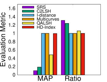
(a) Dataset: SIFT10K

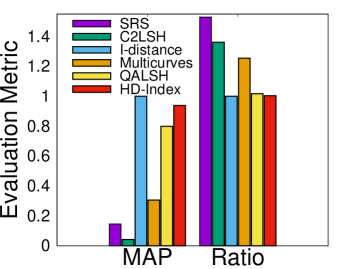
(b) Dataset: Audio

Figure 1: Comparing MAP with approximation ratio ($k=10$).

We next analyze another class of techniques that rely on the use of space-filling curves (such as Hilbert or Z-order) [59] for indexing high-dimensional spaces [66, 51, 46, 42, 40]. Although devoid of theoretical guarantees, these methods portray good retrieval efficiency and quality. The main idea is to construct single/multiple single-dimensional ordering(s) of the high-dimensional points, which are then indexed using a standard structure such as B+-tree for efficient querying. These structures are based on the guarantee that points closer in the transformed space are necessarily close in the original space as well. The vice versa, however, is not true and serves as the source of inaccuracy.

The leaf node of a B+-tree can either store the entire object which improves efficiency while hampering scalability, or store a pointer to the database object which improves scalability at the cost of efficiency. Hence, these methods do not scale gracefully to high-dimensional datasets due to their large space requirements as only a few objects can fit in a node.

In light of the above discussion, the need is to design a scheme that congregates the best of both the worlds (one-dimensional representation of space-filling curves with hierarchical pruning of B+-trees with leaves modified as explained later) to ensure both efficiency and scalability.

To this end, in this paper, we propose a hybrid index structure, HD-Index (High-Dimensional Index). We focus on solving the kANN query for large disk-resident datasets residing in extremely high-dimensional spaces.

We first divide the $\nu$-dimensional space into disjoint partitions. For each lower-dimensional partitioned space, we construct a hierarchical tree structure using the Hilbert space-filling curve orderings. We then propose a novel design called RDB-trees (Reference Distance B+-trees), where instead of object descriptors or pointers, the distances to a fixed set of reference objects are stored in the leaves. While querying, in addition to distance approximation using triangular inequality, we incorporate the use of a more involved lower bounding filter known as the Ptolemaic inequality [30]. Instead of using a single reference object, it approximates the distance using a pair of reference objects. Although costlier to compute, it yields tighter lower bounds. The novel design of RDB-tree leaves allows application of these filtering techniques using the reference objects easily.

Contributions. In sum, our contributions in this paper are:

• We propose a novel, scalable, practical, and yet simple indexing scheme for large extremely high-dimensional Euclidean spaces, called HD-Index (Sec. 3).

• We design a novel structure called RDB-tree with leaves designed to store distances to reference objects for catering to extremely high-dimensional spaces (Sec. 3.2).

• We devise an efficient and effective querying algorithm (Sec. 4) that leverages lower-bounding filters to prune the search space.

• We advocate the use of mean average precision or MAP (Def. 3) as a better metric to benchmark techniques in terms of quality of the retrieved top-$k$ objects, instead of the approximation ratio, especially in high-dimensional spaces. We motivate the need of MAP in real-world applications through an actual information retrieval application, that of image search (Sec. 5.5).

• Through an in-depth empirical analysis (Sec. 5), we show that HD-Index scales gracefully to massive high-dimensional datasets on commodity hardware, and provides speed-ups in running time of up to orders of magnitude, while providing significantly better quality results than the state-of-the-art techniques.

2 Background

2.1 Preliminaries

We consider a dataset $\mathcal{D}$ with $n=|\mathcal{D}|$ $\nu$-dimensional points spanning a vector space. Given a query $q=(q^{1},\dots,q^{\nu})$, and the Euclidean distance function $d$ ($L_{2}$ norm), the k-nearest neighbor (kNN) query is to retrieve the set $T\subset\mathcal{D},|T|=k$ of $k$ nearest neighbors of $q$ from $\mathcal{D}$ such that $\forall o_{i}\in T,\forall o_{j}\notin T,d(q,o_{i})<d(q,o_{j})$. The approximate k-nearest neighbor (kANN) problem relaxes the strict requirement and aims to retrieve a set $A$ of size $k$ that contains close neighbors of $q$.

We next describe two quality metrics to assess the quality of the retrieved kANN answer set. Suppose the true $k$ nearest neighbors of $q$ are $T_{k}=\{o_{1},\dots,o_{k}\}$ in order, i.e., $o_{1}$ is closest to $q$, then $o_{2}$, and so on. Assume that the approximate $k$ nearest neighbors returned are $A_{k}=\{o^{\prime}_{1},\dots,o^{\prime}_{k}\}$, again, in order.

Definition 1 (Approximation Ratio)

The approximation ratio $c\geq 1$ is simply the average of the ratio of the distances:

$$c=\frac{1}{k}.\sum_{i=1}^{k}\frac{d(q,o^{\prime}_{i})}{d(q,o_{i})}$$ (1)

Definition 2 (Average Precision)

Consider the $i^{\text{th}}$ returned item $o^{\prime}_{i}$. If $o^{\prime}_{i}$ is not relevant, i.e., it does not figure in the true set at all in any rank, its precision is $0$. Otherwise, the recall at position $i$ is captured. If out of $i$ items $o^{\prime}_{1},\dots,o^{\prime}_{i}$, $j$ of them figure in the true set, then the recall is $(j/i)$. The average of these values for ranks $1$ to $k$ is the average precision at $k$, denoted by $AP@k$:

$$AP@k=\frac{1}{k}.\sum_{i=1}^{k}\left[I_{o^{\prime}_{i}\in T_{k}}\cdot(j/i)\right]$$ (2)

$I$ is the indicator function: $I=1$ if $o^{\prime}_{i}\in T_{k}$; and $0$ otherwise.

The AP function, thus, prefers correct answers at higher ranks.

Definition 3 (Mean Average Precision)

The mean average precision, denoted by $MAP@k$, is the mean over $AP@k$ values for $Q$ queries:

$$MAP@k=\frac{1}{Q}.\sum_{\forall i=1}^{Q}AP@k(q_{i})$$ (3)

AP and, thus, MAP lie in the range $[0,1]$.

Example 1

Suppose the true ranked order for a query is $\{o_{1},$ $o_{2},o_{3}\}$. Consider $A_{1}=\{o_{4},o_{3},o_{2}\}$. Since $o_{4}$ is not relevant, its precision is $0$. Next, for rank $2$, only $o_{3}$ is relevant. Thus, the precision is $1/2$. Similarly, the precision at $o_{2}$ is $2/3$. The AP, therefore, is $(0+1/2+2/3)/3=0.39$.

The AP for the same set of returned elements but in a different ranked order, $A_{2}=\{o_{3},o_{2},o_{4}\}$, is $(1+1+0)/3=0.67$.

Hence, the MAP for $A_{1}$ and $A_{2}$ is $(0.39+0.67)/2=0.53$.

2.2 Related Work

The problem of nearest neighbor searches, more popularly known as the kNN query, has been investigated by the database community for decades. The basic technique of scanning the entire data does not scale for large disk-resident databases and, consequently, a host of indexing techniques (e.g., R-tree [28] and M-tree families [21]) have been designed to efficiently perform the kNN query [14, 61].

2.2.1 Hierarchical Structures

The R-tree family of structures builds a hierarchy of data objects with the leaf pages containing the actual data points. In each level, the MBR (minimum bounding rectangle) corresponding to the internal node covers all its children nodes. The branching factor indicates how many children nodes can be packed within one disk page. The MBRs can be hyper-rectangular (R-tree [28], R*-tree [9]) or hyper-spherical (SS-tree [72]) or mixed (SR-tree [38]).

Unfortunately enough, for datasets having a large dimensionality, the infamous “curse of dimensionality” [14] renders almost all these hierarchical indexing techniques inefficient and linear scan becomes the only feasible solution [71]. Structures such as the VA-file [71] have, therefore, been designed to compress the data and perform the unavoidable linear scan faster. Techniques to particularly handle the problem of high dimensionality have also been proposed (e.g., the pyramid technique [11], iMinMax [55], iDistance [73], etc.). These structures map a high-dimensional point to a single number and then index that using a B+-tree [22]. A specialized hierarchical structure X-tree [12], on the other hand, adjusts itself with growing dimensionality. In the extreme case, it resembles a simple flat file and the searching degrades to that of a linear scan. To beat the curse of dimensionality, compression through quantization has also been employed. A-tree [60] uses a fixed number of bits per dimension to quantize the data, thereby enabling packing of more children nodes in an internal node. IQ-tree [10] uses different number of quantization bits depending on the number of points in a data MBR and is restricted to only two levels of hierarchy before it indexes the leaf pages directly. Both of them in the end, however, produce the exact correct answer. A survey of such high-dimensional techniques, especially in the context of multimedia databases, is available at [15].

Hierarchical index structures of the M-tree family [21] exploit the property of triangular inequality of metric distances. These structures do not need the vector space representation of points and work directly with the distance between two points. Nevertheless, at high dimensions, the Euclidean distance itself tends to lose its meaning [14] and these structures fail as well.

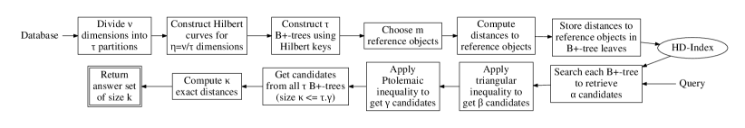
Figure 2: Overview of our approach.

2.2.2 Reference Object-Based Structures

Instead of hierarchical tree-based structures, another important line of research has been the use of reference objects or landmarks or pivots [18, 56]. Certain database points are marked as reference objects and distance of all other points from one or more of these reference objects are pre-computed and stored. Once the query arrives, its distance to the reference objects are computed. Using the triangular inequality (based on the assumption that the underlying distance measure is a metric), certain points can be pruned off without actually computing their distance to the query. AESA [58, 68] and LAESA [52] use the above generic scheme.

Marin et al. [50] employed clustering and the cluster representatives were used as reference objects. Amato et al. [7] proposed inverted distance mappings from a set of representative points based on the premise that in a metric space, if two objects are close to each other, then the relative ordering of the data points from these two objects would also be similar. Chen et al. [20] used representative objects to obtain a vector of distances. The one-dimensional ordering of these vectors were then indexed using a B+-tree.

The choice of representative points has been governed by various factors such as maximizing distance to the already chosen set [16, 18], maximizing the minimum distance among themselves [23], location on the boundary of the dataset [36], whether they are outliers [17], using a nearest neighbor distance loss function [29], minimizing the correlation among themselves [41], or through a sample of queries [67]. Chen et al. [20] included a nice survey of methods to choose representative objects.

2.2.3 Space-Filling Curves

Space-filling curves [59, 14] provide an intuitive way of approximating the underlying data space by partitioning it into grid cells. A one-dimensional ordering is then imposed on the grid cells such that the resultant curve covers each and every grid cell exactly once. The sequence of an occupied grid cell according to the curve is its one-dimensional index. The multi-dimensional points are indexed by the one-dimensional index of the grid cell it occupies. The basic property of these curves ensure that when two points are close in the one-dimensional ordering, they are necessarily close in the original high-dimensional space. The reverse may not be true, though, due to the “boundary” effects where the curve visits a neighboring cell after a long time. Among the different types of space-filling curves, the Hilbert curve is considered to be the most appropriate for indexing purposes [37].

To diminish the boundary effects, the use of multiple space-filling curves have been incorporated. Deterministic translation vectors were used by [42] whereas [62] used random transformation or scaling of data points. Valle et al. [66] proposed an alternative way where different subsets of the dimensions are responsible for each curve. This helps to reduce the dimensionality of the space handled by each curve. Different B+-trees, each corresponding to a particular Hilbert curve, were built. When a query point arrives, the nearest neighbor searches in the different B+-trees aggregate the points. Finally, the approximate nearest neighbors are chosen from this aggregated set.

2.2.4 Locality-Sensitive Hashing

The locality-sensitive hashing (LSH) family [34] of randomized algorithms adopt a completely different approach. The database points are probabilistically hashed to multiple hash tables. The hash functions follow two crucial properties: (1) if two points are close enough, they are very likely to fall in the same hash bucket, and (2) if two points are far-off, they are quite unlikely to fall in the same hash bucket. At run time, the query point is also hashed, and the points falling in the same hash buckets corresponding to each hash table form the candidates. The final approximate nearest neighbor set is chosen from these candidates.

The basic LSH scheme [34] was extended for use in Euclidean spaces by E2LSH [24]. C2LSH [26] was specifically designed on top of E2LSH to work with high-dimensional spaces. LSB-forest [65] builds multiple trees to adjust to the NN distance. Sun et al. devised SRS [64] to have a small index footprint so that the entire index structure can fit in the main memory.

Recently, a query-aware data-dependent LSH scheme, QALSH, has been proposed [33]. The bucket boundaries are not decided apriori, but only after the query arrives in relation to the position of the query. As a result, accuracy improves.

Although the LSH family [34] provides nice theoretical guarantees in terms of running time, space and approximation ratio, however, importantly enough, they provide no guarantees on MAP.

Symbol	Definition
$\mathcal{D}$	Database
$n=|\mathcal{D}|$	Size of database
$o$	Database object
$\nu$	Dimensionality of each object
$\mathcal{P}$	Partition of dimensions
$\tau=|\mathcal{P}|$	Total number of partitions
$\mathcal{H}$	Set of Hilbert curves corresponding to $\mathcal{P}$
$\eta=\nu/\tau$	Dimensionality of each Hilbert curve
$\omega$	Order of Hilbert curve
$\mathcal{B}$	RDB-trees corresponding to $\mathcal{H}$
$\Omega$	Order of RDB-tree leaf
$B$	Disk page size
$\mathcal{R}$	Set of reference objects
$m=|\mathcal{R}|$	Number of reference objects
$q$	Query object
$\alpha$	Number of candidates after RDB-tree search
$\beta$	Number of candidates after triangular inequality
$\gamma$	Number of candidates after Ptolemaic inequality
$\mathcal{C}$	Final candidate set
$\kappa=|\mathcal{C}|$	Size of final candidate set
$\mathcal{A}$	Final answer set
$k=|\mathcal{A}|$	Number of nearest neighbors returned

Table 1: Symbols used in this paper.

2.2.5 In-memory Indexing Techniques

Flann [53] uses an ensemble of randomized KD-forests [63] and priority K-means trees to perform fast approximate nearest neighbor search. Its key novelty lies in the automatic selection of the best method in the ensemble, and allowing identification of optimal parameters for a given dataset. Recently, Houle et al. [31] proposed a probabilistic index structure called the Rank Cover tree (RCT) that entirely avoids the use of numerical pruning techniques like triangle inequality etc., and instead uses rank-based pruning. This alleviates the curse of dimensionality to a large extent.

Proximity graph-based kANN methods [70, 69, 8, 47] have gained popularity, out of which, the hierarchical level based navigable small world method HNSW [48] has been particularly successful.

Quantization based methods aim at significantly reducing the size of the index structure, thereby facilitating in-memory querying of approximate $k$-nearest neighbors. The product quantization (PQ) method [35] divides the feature space into disjoint subspaces and quantize them independently. Each high-dimensional data point is represented using just a short code composed of the subspace quantization indices. This facilitates efficient distance estimation. The Cartesian K-means (CK-Means) [54] and optimized product quantization (OPQ) [27] methods were proposed later as improvements and a generalization of PQ respectively.

Despite their attempt to reduce the index structure size, the techniques discussed above find difficulty in scaling to massive high-dimensional databases on commodity hardware, and instead require machines possessing a humongous amount of main memory.

There have been many other indexing schemes built specifically for ANN queries [13, 25, 32, 39, 43, 44, 45].

2.2.6 Representative Methods

For comparison, we choose the following representative methods: iDistance [73] (as an exact searching technique), Multicurves [66] (hierarchical index using space-filling curves), SRS [64] (low memory footprint), C2LSH [26] (low running time), QALSH [33] (data-dependent hashing with high quality), OPQ [27] (product quantization), and HNSW [48] (graph-based method) since they claim to outperform the other competing methods in terms of either running time, or space overhead, or quality.

3 HD-Index Construction

Algorithm 1 HD-Index Construction

Input: Dataset $\mathcal{D}$ of size $n$ and dimensionality $\nu$
Output: Index HD-Index

1:  $\mathcal{R}\leftarrow$ set of reference objects $\triangleright$Sec. 3.3

2:  $rdist\leftarrow$ dist($\forall\mathcal{R}_{i},\forall\mathcal{D}_{j}$)

3:  $\mathcal{P}\leftarrow$ partition of dimensions $\triangleright$equal and contiguous

4:  $\tau=|\mathcal{P}|$; $\eta=\nu/\tau$

5:  for $i\leftarrow 1$ to $\tau$ do

6:     $\mathcal{P}_{i}\leftarrow$ dimensions $i.\eta$ to $(i+1).\eta-1$

7:     $\mathcal{H}_{i}\leftarrow$ Hilbert($\mathcal{P}_{i},\omega$) $\triangleright$Sec. 3.1

8:     Insert $\mathcal{D}_{j}$ with key $HK(\mathcal{D}_{j})$ into RDB-tree $\mathcal{B}_{i}$ $\triangleright$Sec. 3.2

9:     for $\forall\mathcal{D}_{j}$ in each leaf of $\mathcal{B}_{i}$ do

10:        Store $rdist(\mathcal{D}_{j},\forall\mathcal{R}_{i})$

In this section, we describe in detail the construction of our index structure, HD-Index (Algo. 1). Fig. 2 shows the overall scheme of our method. We use the terminology listed in Table 1.

(a) Dim 1-2

(b) Dim 3-4

(c) Modified RDB-trees.

Figure 3: Hilbert keys and resulting RDB-trees for the example in Table 2.

Since we are specifically targeting datasets in high-dimensional vector spaces, we first divide the entire dimensionality into smaller partitions. A Hilbert curve is then passed through each partition. The resultant one-dimensional values are indexed using a novel structure called RDB-tree. While the upper levels of a RDB-tree resembles that of a B+-tree, the leaves are modified.

We next explain each of the fundamental steps in detail.

3.1 Space-Filling Curves

The total number of dimensions $\nu$ is first divided into $\tau$ disjoint and equal partitions. Although the partitioning can be non-equal and/or overlapping as well, we choose an equal and contiguous partitioning scheme due to two reasons: (1) it is simpler, and (2) the other partitioning schemes do not give any tangible benefit since we assume that the dimensions are independent. The claim is empirically verified in Sec. 5.2.1.

For each partition, a Hilbert curve, catering to $\eta=\nu/\tau$ dimensions, is constructed using the Butz algorithm [19]. The order of a Hilbert curve specifies the number of bits used to describe every dimension. Thus, if the order is $\omega$, each dimension is divided into $2^{\omega}$ equal grid partitions. The single-dimensional value of an object in the Hilbert curve ordering is called its Hilbert key.

As an example, consider the $4$-dimensional dataset of $8$ objects shown in Table 2. The dimensions are broken into two partitions, 1-2 and 3-4. The Hilbert curve for each of these partitions is shown in Fig. 3a and Fig. 3b. The Hilbert keys for the objects are obtained by considering the sorted order along the curve, and are shown in the last two columns of Table 2.

Multiple Hilbert curves are beneficial in not only reducing the dimensionality but also tackling the “boundary” effect. It is unlikely that nearby objects will have far-off Hilbert keys in all the partitions. For example, in Fig. 3a, $O_{7}$ and $O_{1}$ having adjacent Hilbert keys are nearby in space, while objects $O_{8}$ and $O_{4}$, despite being close in space, have far-off Hilbert keys. However, in Fig. 3b, $O_{8}$ and $O_{4}$ have adjacent Hilbert keys. Objects $O_{7}$ and $O_{1}$ continue to be close in both the cases. It is enough for an object that is a nearest neighbor to have a close Hilbert key in only one partition to be chosen as a candidate.

Object	Dim 1	Dim 2	Dim 3	Dim 4	HK 1	HK 2
$O_{1}$	0.20	0.74	0.68	0.73	3	5
$O_{2}$	0.84	0.34	0.49	0.81	6	5
$O_{3}$	0.97	0.64	0.32	0.93	5	3
$O_{4}$	0.42	0.86	0.12	0.82	4	2
$O_{5}$	0.62	0.09	0.56	0.07	7	7
$O_{6}$	0.84	0.59	0.49	0.73	5	4
$O_{7}$	0.05	0.43	0.52	0.82	2	6
$O_{8}$	0.40	0.24	0.10	0.64	1	1
$Q$	0.18	0.87	0.76	0.23	-	-

Table 2: Running example ($O_{3},O_{7}$ are reference objects).

3.2 RDB-trees

Corresponding to the $\tau$ Hilbert curves, $\tau$ RDB-trees are next constructed using the Hilbert keys of the objects.

The reasons for not adapting the standard B+-tree leaf structure are as follows. If only the pointers to the actual objects are stored in the leaf, then accessing $\alpha$ objects require $\alpha$ random disk accesses. The number of such random disk accesses can be reduced by storing the entire object descriptor (and not a pointer to it) in the leaf itself. However, in high dimensions, the number of objects that can be stored in the leaf is extremely low. For example, assuming a page size of 4 KB, only $4$ objects of dimensionality $128$ can fit in a page, where each dimension is of $8$ bytes. Hence, none of these designs is suitable for high-dimensional spaces.

We, therefore, modify the leaves to store distances to reference objects. Reference objects are specially designated objects from the dataset that are used to quickly obtain approximate distances to the query. We explain the querying process using reference objects in Sec. 4 and how they are chosen in Sec. 3.3. In this section, we assume that the set of reference objects $\mathcal{R}$ of size $m$ is known.

For each object, the distance to all the $m$ reference objects are stored as part of its description. Hence, as long as $m<\nu$, where $\nu$ is the dimensionality of the object, more number of objects can fit in a page of RDB-tree than a B+-tree (assuming that the storage requirement for a distance value is the same as that for a dimension).

In Sec. 5, we show that even for extremely large datasets, a reference set size of $10$ suffices. Thus, the reduction in number of random disk accesses required to retrieve the same number of candidate objects for a $128$-dimensional space is almost $13$ times.

Dataset	Dimen-	Hilbert	Dimensions	Reference	RDB-tree
	sions, $\nu$	order, $\omega$	per curve, $\eta$	objects, $m$	leaf order, $\Omega$
SIFTn	128	8	16	10	63
Yorck	128	32	16	10	36
SUN	512	32	64	10	13
Audio	192	32	24	10	28
Enron	1369	16	37	10	18
Glove	100	32	10	10	40

Table 3: RDB-tree leaf order (page size = 4 KB).

The order of the RDB-tree leaves is computed as follows. Storing the Hilbert key of an object requires $\eta.(\omega/8)$ bytes since for each of the $\eta$ dimensions, $\omega/8$ bytes describe the key. The distances to $m$ reference objects requires $4.m$ bytes of storage. The pointer to the complete object descriptor consumes a further $8$ bytes. Thus, if there are $\Omega$ objects in a RDB-tree, its storage requirement is $(\eta.(\omega/8)+4.m+8).\Omega$ bytes. Adding the overheads of left and right pointers ($8$ bytes each) to the sibling leaves and an indicator byte to indicate that it is a leaf, if the page size is $B$ bytes,

$$(\eta\cdot(\omega/8)+4\cdot m+8)\cdot\Omega+16+1\leq B$$ (4)

The order $\Omega$ is the largest integer that satisfies Eq. (4). Table 3 lists the RDB-tree leaf orders for the datasets we use.

Assuming that the reference objects chosen are $O_{3}$ and $O_{7}$, the RDB-trees constructed using the Hilbert keys are shown in Fig. 3c. The leaves contain actual distances to $O_{3}$ and $O_{7}$ respectively.

3.3 Reference Object Selection

In order to avoid the actual distance computation between an object and the query at run time, reference objects are used to approximate the distance and quickly filter out objects. We describe the details of how the distance is approximated later in Sec 4. In this section, we describe the desirable properties of the set of reference objects $\mathcal{R}$ and how they are chosen.

The nature of the distance approximation is such that the closer a reference object is to the query, the better is the approximation. Hence, the set of reference objects should be well spread in the data space. This ensures that no matter where the query is located, there is at least one reference object that is not too far away from it and, hence, the approximation of distances to other objects using this reference object is good. The above objective assumes that any reference object can be used to approximate the distance for any other object. In other words, the purview of every reference object is the entire dataset. Thus, the distance from an object to all the reference objects must be pre-computed and stored.

Considering the above issues, a good choice for reference object selection is the sparse spatial selection (SSS) algorithm [56]. The method first estimates the largest distance, $d_{max}$, between any two objects in the database using the following heuristic. A random object is selected and its farthest neighbor is found. This neighbor is then selected and the process of finding the farthest object is repeated. The process continues till convergence or for a fixed number of iterations.

Once $d_{max}$ is estimated, an object is chosen randomly as the first reference object. In every iteration, the dataset is scanned till an object whose distance to all the previously selected reference objects is greater than a fraction $f$ of $d_{max}$ is found. This object is added to the set $\mathcal{R}$. The process is continued till $|\mathcal{R}|=m$.

The SSS dynamic (SSS-Dyn) [18] method extends the above by continuing the process beyond the first $m$ iterations. For every new object that satisfies the fraction $f$ condition, it chooses a victim from the current set. The victim is the one that contributes the least towards approximating the distance between a set of (pre-selected and fixed) object pairs. If the contribution of the new object is better than the victim, it replaces the victim as a reference object. This goes on till there are no more objects that satisfy the $f$ condition. The choice of the method is discussed in Sec. 5.2.2.

The number of reference objects, $m$, determines the amount of pre-processing and storage required for each database object. More importantly, since the RDB-tree leaves store the distances to these $m$ reference objects, it determines the order of the RDB-trees at the leaf level as shown in Eq. (4).

The offline index building phase is completed with the construction of the $\tau$ RDB-trees. We refer to this union of the $\tau$ RDB-trees, each storing $n$ Hilbert key values of the database points from $\eta$-dimensional sub-spaces, with the leaves storing the distances to $m$ reference objects, as the HD-Index (High-Dimensional Index).

3.4 Tuning of Parameters

The order $\omega$ of the Hilbert curve should be such that there is no large loss in the representation after the quantization using $\omega$ bits. Therefore, it depends on the domain from which the individual dimensions of the descriptors draw their value. Table 4 shows the details of the datasets including their domain sizes while Table 3 lists the Hilbert curve orders and other parameters.

If the number of partitions $\tau$ is more, then the larger number of Hilbert curves increases the number of RDB-tree searches, thereby increasing the overall searching time. However, simultaneously, $\eta$ decreases which results in better approximation by the Hilbert curve, thereby increasing the accuracy. Hence, the value of $\tau$ (or equivalently, $\eta$) provides a handle to balance the trade-off between running time and accuracy. We discuss the tuning of these parameters experimentally in Sec. 5.

From our experiments, we observed that the effect of varying $f$ on the overall quality and efficiency of the reference object selection method is minimal. Hence, we chose $f=0.3$.

3.5 Analysis

3.5.1 Time and Space Complexities

We first analyze the index construction time of HD-Index.

Estimating $d_{max}$ for reference object selection requires $O(n)$ time since the iterations are continued for at most a (constant) threshold number of times. In each iteration, a potential reference object is checked against all the $O(m)$ existing reference objects. Assuming a worst case of $O(n)$ potential reference objects, the total time for $m$ iterations is $O(m^{2}.n)$.

Computing the distances between the objects and the references having dimensionality $\nu$ consumes $O(m.n.\nu)$ time.

Mapping a single point to a Hilbert key of order $\omega$ catering to a dimensionality of $\eta$ requires $O(\omega.\eta)$ time. Thus, the time for $n$ objects is $O(\omega.\eta.n)$. The RDB-tree construction requires $O(n.\log_{\theta}n)$ time where $\theta$ is the branching factor of the internal nodes. Since there are $\tau=\nu/\eta$ RDB-trees, the total time for this phase is $O((\omega.\eta.n+n.\log_{\theta}n).\tau)=O(\nu.\omega.n+\tau.n.\log_{\theta}n)$.

The total construction time of HD-Index is, therefore, $O(m^{2}.n+m.n.\nu+\nu.\omega.n+\tau.n.\log_{\theta}n)$.

We next analyze the space requirements for HD-Index. The original data objects require $O(n.\nu)$ storage. In each of the $\tau$ RDB-trees and for each of the database objects, the following are stored: (1) Hilbert key composed from $\eta$ dimensions, (2) pointer to the original object, and (3) distances to $m$ reference objects. This requires a total of $O(\tau.n.(\eta+O(1)+m))=O(n.\nu+\tau.n.m)$ space. The rest of the RDB-tree requires $O(n.\eta)$ space to store the $O(n)$ internal nodes consisting of Hilbert keys. Hence, the total space requirement of HD-Index is $O(n.\nu+n.m.\tau)$.

3.5.2 Discussion

In practice, $\omega$, $\tau$, the height of the RDB-tree ($\log_{\theta}n$), and $m\ll n$ are small constants (as verified experimentally in Sec. 5 as well). Hence, the construction time and space complexities of HD-Index are essentially $O(n.\nu)$, which is the size of the input. This linear scaling factor allows HD-Index to scale gracefully to extremely large datasets and high dimensionality.

3.6 Handling Updates

In this section, we describe how updates are handled. We only discuss insertions since deletions can be handled by simply marking the object as “deleted” and not returning it as an answer. Since B+-trees are naturally update-friendly, inserting new points in a RDB-tree requires a very small amount of computation: the Hilbert key of the new object and its distances to reference objects.

Although the set of reference objects may change with insertions, since the performance with even random reference objects are quite close in quality to a carefully chosen set (Sec. 5.2.2), we do not re-compute the set $\mathcal{R}$ with every new insertion. Also, the number of updates, if any, are generally insignificant with respect to the total number of objects and, hence, there is little merit in updating the reference set.

4 Querying

We next describe the kNN search procedure for a query object $q$ residing in the same $\nu$-dimensional Euclidean space (Algo. 2).

Algorithm 2 kNN Query using HD-Index

Input: Query $q$, Number of nearest neighbors $k$
Output: Approximate kNN $\mathcal{A}$

1:  for $i\leftarrow 1$ to $\tau$ do

2:     $q_{i}\leftarrow$ dimensions of $q$ according to $\mathcal{P}_{i}$

3:     $k_{i}\leftarrow$ Hilbert key of $q_{i}$

4:     $C^{1}_{i}\leftarrow\alpha$ nearest objects of $k_{i}$ from $\mathcal{B}_{i}$

5:     for $j\leftarrow 1$ to $\alpha$ do

6:        Compute $\tilde{d}_{\triangle}(q,C^{1}_{i}(j))$ using Eq. (5)

7:     $C^{2}_{i}\leftarrow\beta$ nearest objects from $\tilde{d}_{\triangle}(q,C^{1}_{i}(j))$

8:     for $j\leftarrow 1$ to $\beta$ do

9:        Compute $\tilde{d}_{\square}(q,C^{2}_{i}(j))$ using Eq. (6)

10:     $C^{2}_{i}\leftarrow\gamma$ nearest objects from $\tilde{d}_{\square}(q,C^{2}_{i}(j))$

11:  $\mathcal{C}\leftarrow\cup_{i=1}^{\tau}C^{2}_{i}$

12:  for $j\leftarrow 1$ to $\kappa=|\mathcal{C}|$ do

13:     Access object $\mathcal{C}(j)$

14:     Compute actual distance $d(q,\mathcal{C}(j))$

15:  $\mathcal{A}\leftarrow k$ nearest objects from $d(q,\mathcal{C}(j))$

16:  return  $\mathcal{A}$

The querying process follows three broad steps: (i) retrieving candidate objects from the RDB-trees using the Hilbert keys, (ii) refining the candidate set by applying distance approximation inequalities, and (iii) retrieving the $k$ approximate nearest neighbors by computing the actual distances from the candidates.

We next describe each of them in detail.

4.1 Retrieving Candidates from RDB-trees

The $\nu$ dimensions of the query $q$ are divided into $\tau$ groups according to the same partitioning scheme $\mathcal{P}$ as the dataset.

For each of these $\tau$ partitions, the corresponding RDB-tree $\mathcal{B}_{i}$ is searched with the Hilbert key of $q$ associated with the dimensions $\mathcal{P}_{i}$. The nearest $\alpha$ candidate objects are returned. These objects are close in the space represented by $\mathcal{P}_{i}$ and, therefore, have the potential to be close in the entire $\nu$-dimensional space as well.

Returning to our example in Fig. 3, assuming $\alpha=2$, the first RDB-tree returns $O_{1},O_{4}$ while the second one returns $O_{5},O_{7}$.

4.2 Refining Candidates using Approximation

The $\alpha$ objects are then successively refined by applying two distance approximation schemes—triangular inequality and Ptolemaic inequality—using the reference objects. As a pre-requisite, the distance of query $q$ to all the $m$ reference objects are computed.

The triangular inequality using the $i^{\text{th}}$ reference object $\mathcal{R}_{i}$ lower bounds the distance between the query $q$ and an object $o$ as follows:

$$d(q,o)\geq\tilde{d}_{\triangle}(q,o)_{i}=|d(q,\mathcal{R}_{i})-d(o,\mathcal{R}_{i})|$$

Using $m$ reference objects produces $m$ lower bounds for an object $o$. The best lower bound is the one that is maximal and is, therefore, considered as the approximate distance of $o$ from $q$:

$$\tilde{d}_{\triangle}(q,o)=\max_{\forall\mathcal{R}_{i}\in\mathcal{R}}\tilde{d}_{\triangle}(q,o)_{i}$$ (5)

Using this approximate distance, the $\alpha$ candidates are sorted and the $\beta$ nearest ones to $q$ are chosen as the next set of candidates for the application of the next distance approximation, the Ptolemaic inequality [30], which is respected by the Euclidean distance.

The Ptolemaic inequality uses two reference objects $\mathcal{R}_{i}$ and $\mathcal{R}_{j}$ to lower bound the distance:

$$d(q,o)\geq\tilde{d}_{\square}(q,o)_{i,j}=\frac{|d(q,\mathcal{R}_{i}).d(o,\mathcal{R}_{j})-d(q,\mathcal{R}_{j}).d(o,\mathcal{R}_{i})|}{d(\mathcal{R}_{i},\mathcal{R}_{j})}$$

The best (i.e., maximal) lower bound among the $m\choose 2$ possibilities is considered as the approximate distance:

$$\tilde{d}_{\square}(q,o)=\max_{\forall\mathcal{R}_{i},\mathcal{R}_{j}\in\mathcal{R}}\tilde{d}_{\square}(q,o)_{i,j}$$ (6)

The nearest $\gamma$ candidates, chosen from the $\beta$ candidates using Eq. (6), forms the final candidate set from the RDB-tree $\mathcal{B}_{i}$.

The order of applying the inequalities is important as the approximation using Ptolemaic inequality is costlier but better than the triangular inequality.

The $\gamma$ candidates from each $\mathcal{B}_{i}$ are merged to form the final candidate set $\mathcal{C}$. The size of $\mathcal{C}$, denoted by $\kappa$, is at least $\gamma$ (when all the partitions produce the same set) and at most $\tau.\gamma$ (when the partitions produce completely disjoint sets). Thus, $\gamma\leq\kappa\leq\tau.\gamma$.

4.3 Retrieving k Nearest Neighbors

Finally, the complete descriptions of the candidate objects in $\mathcal{C}$ are accessed using the corresponding object pointers from the RDB-trees, and the actual distances from $q$ are computed. The $k$ nearest objects from $\mathcal{C}$ are returned as the kANN answer set $\mathcal{A}$.

4.4 Analysis

4.4.1 Time and Space Complexities

We first analyze the time complexity of the querying phase.

The cost of distance computation from $q$ to all the $m$ reference objects is $O(m.\nu)$.

For each of the $\tau$ partitions, the following costs are paid. Retrieval of $\alpha$ candidates from a RDB-tree requires $O(\log_{\theta}n+\alpha)$ time where $\theta$ is the branching factor of the RDB-tree internal nodes. Computing the triangular inequalities for $\alpha$ candidates using $m$ reference objects takes $O(\alpha.m)$ time due to pre-processing. By using a heap, the nearest $\beta$ candidates are chosen in $O(\alpha.\log\beta)$ time. Subjecting the $\beta$ candidates to Ptolemaic inequalities requires $O(\beta.m^{2})$ time. Finally, $\gamma$ candidates are extracted using a heap in $O(\beta.\log\gamma)$ time. The total cost over $\tau$ partitions is, therefore, $O(\tau.(\log_{\theta}n+\alpha+\alpha.m+\alpha.\log\beta+\beta.m^{2}+\beta.\log\gamma))$.

Computing the actual distances for $\kappa$ candidates requires $O(\kappa.\nu)$ time. Since $\kappa$ is at most $\tau.\gamma$, this phase runs in $O(\tau.\gamma.\nu)$ time.

Adding up the costs of each phase gives the total time.

The extra space overhead is that of $\alpha$ candidates. Since the RDB-trees are processed sequentially, the extra space overhead remains $O(\alpha)$ which is essentially a constant.

Since HD-Index is a disk-based structure, we next analyze the number of random disk accesses needed for a kANN query. The computation of $m$ distances from the query to the reference objects require $O(m)$ disk accesses. However, since $m\ll n$, the reference object set can be assumed to fit in memory and, therefore, no I/O cost is incurred. Assuming the order of a RDB-tree leaf to be $\Omega$, retrieving $\alpha$ objects requires $O(\log_{\theta}n+(\alpha/\Omega))$ disk accesses. The computation of the distance inequalities do not require any more disk access since the distances to the reference objects are stored in the leaves themselves. Computing $\kappa$ exact distances from the candidates require $\kappa=O(\tau.\gamma)$ disk accesses. Hence, the total number of disk accesses is $O(\tau.(\log_{\theta}n+(\alpha/\Omega)+\gamma))$.

4.4.2 Discussion

As shown in Sec. 5, it suffices to have $\alpha\ll n$ for even extremely large datasets. Consequently, $\alpha$, $\beta$ and $\gamma$ are essentially constants in the overall analysis. Since $\omega$ and $m\ll n$ are also small constants, the running time of a kANN query can be summarized as $O(\tau.(\log_{\theta}n+\nu))$, i.e., it is linear on the number of RDB-tree searches, the height of a RDB-tree, and the dimensionality. The extra space consumed during the search is $O(\alpha)$, which is negligible. The number of disk accesses is linear in the number of trees, the height of the trees, and candidate size, thus allowing HD-Index to scale gracefully to large datasets and high-dimensional spaces.

5 Experiments

All the experiments were done using codes written in C++ on an Intel(R) Core(TM) i7-4770 machine with 3.4 GHz CPU, 32 GB RAM, and 2 TB external disk space running Linux Ubuntu 12.04. The results are summarized in Sec. 5.6.

Datasets: We present results on large-scale high-dimensional real-world and benchmark datasets, taken from various publicly available sources [6, 5, 3, 4, 2, 1], as described in Table 4. Our datasets constitute a judicious mix of scale, dimensionality, and domain types.

• The Audio dataset comprises of audio features extracted using Marsyas library from the DARPA TIMIT speech database [2].

• The SUN dataset comprises of extremely high-dimensional GIST features of images [5].

• The SIFT datasets comprise of SIFT features [1] at varying scale.

• The Yorck dataset comprises of SURF features extracted from images in the Yorck project [6].

• The Enron dataset comprises of feature vectors of bi-grams of collection of emails [3].

• The Glove dataset comprises of word feature vectors extracted from Tweets [4].

Dataset	Type	Dimen-	# Objects	Domain	# Queries
		sionality		of values
SIFT10K	Tiny	128	10,000	[0,255]	100
Audio	Small	192	54,287	[-1,1]	10,000
SUN	Small	512	80,006	[0,1]	100
SIFT1M	Medium	128	1,000,000	[0,255]	10,000
SIFT10M	Medium	128	10,000,000	[0,255]	10,000
Yorck	Medium	128	15,120,935	[-1,1]	1,254
SIFT100M	Large	128	100,000,000	[0,255]	10,000
SIFT1B	Large	128	999,494,170	[0,255]	10,000
Enron	Small	1369	93,986	[0,252429]	1,000
Glove	Medium	100	1,183,514	[-10,10]	10,000

Table 4: Datasets.

Note that SIFT and Enron features are integers, while all other datasets possess floating point feature values. The Hilbert curve and RDB-tree orders are shown in Table 3.

Next, we state the methods, their parameters and the evaluation metrics used for obtaining the results.

Methods: We compare HD-Index for effectiveness, efficiency and scalability against a number of representative state-of-the-art methods, namely, Multicurves, C2LSH, SRS, QALSH, OPQ, and HNSW [66, 26, 64, 33, 27, 48]. In addition, we also consider iDistance [73], which is an exact method for kNN queries and will, therefore, always exhibit perfect quality. For all these techniques, we adopt the C++ implementations made available by their authors.

Parameters: The disk page size for the machine on which the experiments were run is $B=4096$ bytes. We set the number of nearest neighbors $k=100$. The parameters for the competing techniques were set as follows: iDistance: initial radius $r=0.01$, $\Delta r=0.01$; Multicurves: $\tau=8$, $\alpha=4096$; C2LSH: approximation ratio $c=2$, interval size $w=1$, false-positive percentage $\beta^{C2LSH}=100/n$, error probability $\delta=1/e$; QALSH: approximation ratio $c=2$, false-positive percentage $\beta^{QALSH}=100/n$, error probability $\delta=1/e$; SRS: algorithm SRS-12, approximation ratio $c=2$, number of 2-stable random projections $m^{SRS}=6$, early termination threshold $\tau^{SRS}=0.1809$, maximum percentage of examined points $t=0.00242$; OPQ: number of subspaces $M=8$; HNSW: number of nearest neighbors $M=10$. The search parameters of OPQ and HNSW were set such that their MAP values were close to those of HD-Index. Note that most of these parameters have been set according to the recommendations by their respective authors.

Evaluation Metrics: We consider the following metrics:

• Quality: We adopt approximation ratio (Def. 1) and MAP@$k$ (Def. 3) to evaluate the quality of the discussed methods.

• Efficiency: We evaluate the efficiency of the methods using the running time of the queries. For fairness, we turn off buffering and caching effects in all the experiments.

• Scalability: To evaluate the scalability, we measure (1) the size and (2) construction time of the index structures, and main memory consumption during (3) index construction and (4) querying.

All the reported values are averages over the entire query set.

5.1 Comments

All the datasets are pre-processed to remove the duplicate points, if any. We used the set of queries provided with the Audio and the SIFT datasets for our experiments. For the datasets where query sets were not provided, namely, SUN, Yorck, Enron, and Glove, we reserved $100$, $1254$, $1000$, and $10000$ random data points respectively as queries. Since the implementations of some of the techniques do not support floating point data, to enable them to run on datasets with floating point feature values, the values are scaled by a sufficiently large number. This is as suggested by the corresponding authors of C2LSH and SRS.

Although it is not a requirement of the algorithms, the publicly available implementations of C2LSH, QALSH, and iDistance load the entire dataset into main memory during the index construction step. Thus, it crashed on our machine for the two largest datasets, SIFT100M and SIFT1B, that require $\sim$52GB and $\sim$520GB of RAM to be loaded respectively. Further, the underlying implementation of R-trees used by SRS suffers from memory leaks. Hence, to enable SRS run on SIFT100M and SIFT1B, as suggested by the authors, these datasets were divided into chunks, indexed separately and then combined together into a single index for the whole dataset. This discussion highlights the importance of purely disk-based methods, as even with today’s hardware, methods using very large amounts of main memory in a single machine to build and load the index structure may not be deemed as scalable.

5.2 Internal Parameter Tuning

Since the HD-Index structure and its querying mechanism uses some parameters, the first set of experiments is performed to determine a good range of their values. This is a critical step. The parameter tuning process follows an order such that the most general parameter, i.e., the one which is independent of other parameters, is tuned first and so on. In general, we follow the intuitive order of first tuning the parameters specific to HD-Index construction followed by those used during querying.

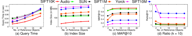
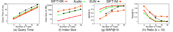
Figure 4: Effect of varying number of reference objects, $m$, on (a) Query time, (b) Index size, (c) MAP@10, and (d) Ratio ($k=10$). Effect of varying number of RDB-trees, $\tau$, on (e) Query time, (f) Index size, (g) MAP@10, and (h) Ratio ($k=10$).

(a) Query Time (SIFT10K)

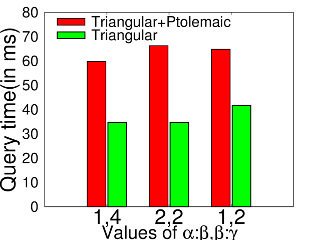
(b) Query Time (Audio)

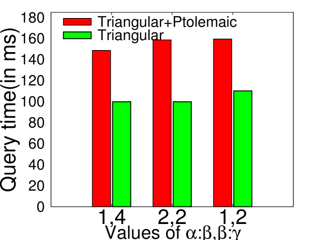
(c) Query Time (SUN)

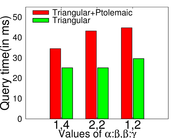
(d) Query Time (SIFT1M)

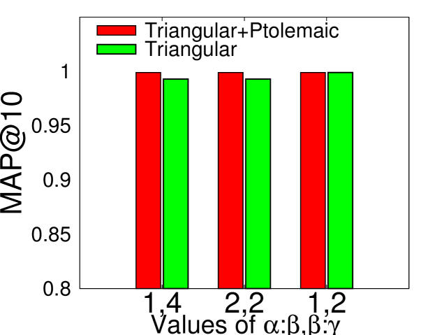
(e) MAP@10 (SIFT10K)

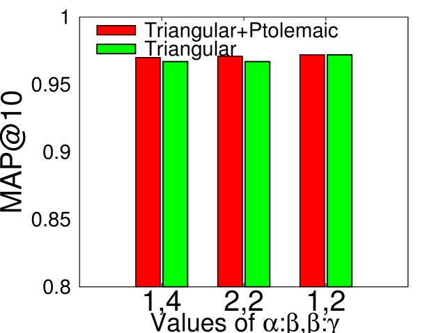
(f) MAP@10 (Audio)

(g) MAP@10 (SUN)

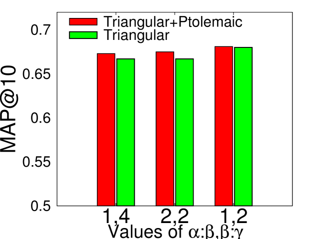
(h) MAP@10 (SIFT1M)

Figure 5: Effect of the filtering mechanism (either triangular inequality alone or a combination of triangular and Ptolemaic inequalities) on query time (a-d) and MAP@10 (e-h) with $\alpha=4096$.

5.2.1 Indexing: Subspace Partitioning Scheme

During the index construction step, HD-Index requires data to be partitioned into different lower dimensional sub-spaces. For ease of use, we sequentially partition the feature space. However, that is not necessary, since HD-Index is not dependent upon a particular partitioning scheme. To substantiate this claim, we perform querying on $100$ indices constructed by randomly partitioning the full space into multiple sub-spaces. The MAP@10 values over the $100$ indices for the different datasets are as follows: (a) SIFT10K: $0.974\pm 0.002$, (b) Audio: $0.934\pm 0.013$, (c) SUN: $0.750\pm 0.010$, (d) SIFT1M: $0.660\pm 0.010$. Considering the small standard deviations and comparable results of MAP@10 for contiguous partitioning (as shown later in Fig. 5e-Fig. 5h), we conclude that quality does not depend significantly on the choice of partitioning scheme.

5.2.2 Indexing: Reference Object Selection Method

As mentioned earlier in Sec. 2.2, there are multiple methods of choosing the reference objects. We have experimented with three algorithms: the random method, where $m$ random objects are chosen as reference objects, SSS and SSS-Dyn. Compared to the other sophisticated methods, even the random reference object selection has comparable accuracy levels. (The MAP values are within 90% of those of SSS). The figures are shown in Fig. 10 in Appendix A.

This indicates that the design of HD-Index by itself is good enough to achieve a high accuracy, and the choice of reference objects is not very critical. The SSS method is faster and has similar MAP values as SSS-Dyn. Also, the larger the dataset, the lesser the difference between the methods. Consequently, we recommend the SSS method as the reference object selection algorithm.

5.2.3 Indexing: Number of Reference Objects

The first important parameter is the number of reference objects, $m$. To effectively tune $m$, we consider the top $6$ datasets of up to medium size from Table 4. Fig. 4a shows that the query time increases in a sub-linear fashion with $m$. The size of the final index (Fig. 4b) grows linearly with $m$ (y-axis in log scale). However, for all the datasets, the quality metrics saturate after $m=10$, with little or no further changes (Fig. 4c and Fig. 4d). Thus, we choose $m=10$ as the recommended number of reference objects. For the rest of the experiments, we use this value.

5.2.4 Indexing: Number of RDB-trees

Next, we analyze the effect of the number of RDB-trees $\tau$ on the different evaluation metrics. We use the top $4$ datasets from Table 4. Figs. 4e and 4f show that, as expected, the running time and the size of the final index grow linearly with increasing $\tau$, for all the datasets. However, Figs. 4g and 4h portray that quality saturates after a while. The MAP@10 values for all the datasets, except SUN, saturates after $\tau=8$. A similar effect is observed for the approximation ratio as well. Thus, we choose $\tau=8$ as the recommended number of RDB-trees. However, for the SUN dataset, which has a very high dimensionality of $\nu=512$, choosing $\tau=8$ makes each Hilbert curve cater to a dimensionality of $\eta=512/8=64$. Consequently, for such a high dimensionality, the MAP performance suffers. The MAP performance increases significantly by using double the number of trees, i.e., $\tau=16$. Hence, while the default value is $\tau=8$, for extremely high dimensional datasets (500+), we recommend $\tau=16$. For datasets where the dimensionality is not a power of $2$, we choose parameters that are as close as possible to the recommended values. Thus, for Enron, we use $\tau=37$ trees, each catering to $\eta=37$ dimensions, while for Glove, we use $\tau=10$ trees, each handling $\eta=10$ dimensions.

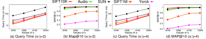
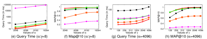
Figure 6: Effect of varying $\alpha$ on query time and MAP@10 with $\alpha/\gamma=2$ (a,b); with $\alpha/\gamma=4$ (c,d); and with $\alpha/\gamma=8$ (e,f); and Effect of varying $\gamma$ on (g) query time and (h) MAP@10 with $\alpha=4096$.

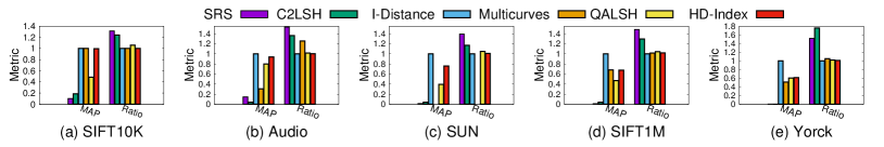
Figure 7: Comparison of MAP@10 and approximation ratio for $k=10$ on different datasets.

5.2.5 Querying: Importance of Ptolemaic Inequality

Having tuned the parameters specific to HD-Index, we next analyze the effect of parameters associated with the querying mechanism. We first evaluate the effect of the lower bounding filters – triangular and Ptolemaic inequalities. Fig. 5 presents a detailed analysis of using (1) just the triangular inequality, i.e., $\beta=\gamma$ (as explained in Sec. 4.2), and (2) a combination of both triangular and Ptolemaic inequalities, for an initial candidate set size of $\alpha=4096$ on different datasets. While it is clear from Figs. 5e-5h that MAP@10 obtained using a combination of triangular and Ptolemaic inequality filters is always better when compared to using the triangular inequality alone, the gain is not significant under all scenarios. Notable gains are observed only when we use $\alpha/\beta=1$ and $\beta/\gamma=4$ for the combined filtering process, and $\alpha/\gamma=4$ for triangular inequality alone. This is because tighter lower bounds using Ptolemaic inequality are more robust to large reductions during the filtering process. On the other hand, it is evident from Figs. 5a- 5d that the running times obtained using the combined filters are consistently $1.5$–$2$ times slower when compared to using the triangular inequality alone. A similar pattern is followed for different $\alpha$ values as well (additional results are shown in Appendix B).

In sum, although the use of Ptolemaic inequality results in better MAP, the gain in quality is not significant in majority of the cases when compared to the increase in query time, which almost doubles. Therefore, it is more prudent to use the triangular inequality alone to trade a little amount of quality (loss in MAP) for a much higher query efficiency. Thus, we henceforth choose triangular inequality alone as the recommended choice of lower bounding filter.

As an alternate analysis, although the application of Ptolemaic inequality is slower, importantly, it does not affect the number of disk I/Os. Since all the $\alpha$ candidates are processed in main memory without the need to access the disk, Ptolemaic inequality only requires more CPU time. Thus, if the performance metric of an application is the number of disk I/Os (instead of the wall clock running time), it is better to use Ptolemaic inequality since it produces better quality results using the same number of disk accesses.

5.2.6 Querying: Filter Parameters

Since we do not use the Ptolemaic inequality, the intermediate filter parameter $\beta$ is not needed any further. We next fine tune the other filter parameters $\alpha$ and $\gamma$ by plotting (Fig. 6) MAP@10 and running time for the top $5$ datasets from Table 4. Figs. 6a, 6c and 6e show that, as expected, the running time scales linearly with increase in $\alpha$. However, Figs. 6b,  6d and 6f portray that the quality saturates after a while (after $\alpha=4096$). Thus, we choose $\alpha=4096$ as the recommended value.

However, for SIFT1M and Yorck, $\alpha=4096$ is not sufficient since these datasets are extremely large. MAP improves when double the value, i.e., $\alpha=8192$ is used and saturates beyond that. Hence, for very large datasets, we recommend $\alpha=8192$.

Having fixed $\alpha$, we analyze the MAP@10 and running times for all the datasets with varying $\gamma$. Fig. 6g shows that the running time scales linearly with increase in $\gamma$. However, once again, MAP@10 saturates after $\gamma=1024$ for all the datasets. Thus, we choose $\gamma=1024$, and $\alpha/\gamma=4$, as the recommended values.

5.2.7 Robustness with Number of Nearest Neighbors

We also evaluate MAP@$k$ and running times of the techniques with varying $k$ on the tiny, small and medium datasets (results in Appendix C). While the running times of the other techniques increase with $k$, it remains almost constant for HD-Index and Multicurves. This is mainly due to the design of these structures where $\alpha$ candidates are selected and then refined to return $k$ answers in the end. Since $\alpha>k$, the running times are not affected by $k$.

5.2.8 Limitations

It needs to be noted that the current parameter tuning of HD-Index is almost purely empirical. In future, we would like to analyze the parameters from a theoretical stand-point and understand what values can be reasonable for a given dataset.

Also, if the dataset really exhibits ultra-high dimensionality (in order of hundreds of thousands), then HD-Index is unable to process the queries efficiently since there are too many B+-trees. However, on that note, we would also like to clarify that to the best of our knowledge, there is no disk-based database indexing method that can really handle such ultra-high dimensionality. However, our method can be easily parallelized and/or distributed with little synchronization steps due to its nature of building and querying using multiple independent RDB-trees.

For small datasets, HD-Index is not as efficient as some of the other techniques (as explained in more detail in Sec. 5.4). However, as the dataset size increases, it scales better.

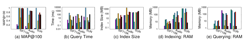
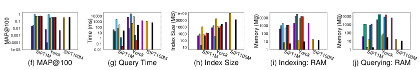
Figure 8: Comparison on different parameters for $k=100$ using small datasets (a-e), larger datasets (f-j), and text datasets (k-o).

5.3 Quality Metrics

With the HD-Index parameters fine-tuned, we evaluate the two quality metrics, MAP@$k$ and approximation ratio vis-à-vis the other methods. It is evident from Fig. 7a-7e that even for good approximation ratios ($c\leq 1.5$), MAP values can be surprisingly and significantly low (MAP $\leq 0.15$). Moreover, with increase in dimensionality $\nu$, this effect becomes more and more prominent. For instance, in Fig. 7c, $c=1.15$ and $1.39$ for C2LSH and SRS respectively, while MAP are $0.04$ and $0.01$ respectively.

This analysis highlights a notable limitation of the techniques that possess theoretical guarantees on the approximation ratio as it empirically proves that the ratio loses its significance. Thus, henceforth, we use only MAP@k.

5.4 Comparative Study

In this section, we perform an in-depth comparison of the different methods with respect to three aspects: (a) quality of results, (b) efficiency of retrieval in terms of running time, and (c) scalability in terms of space usage for both main memory and on disk.

5.4.1 Quality

Figs. 8a, 8f, 8k show a comparison of MAP@100 of the different techniques. Being an exact technique, iDistance possesses the best quality, with a MAP of $1$. However, it is neither efficient nor scalable. Table 5 shows that HD-Index significantly outperforms all the other techniques except HNSW and OPQ in terms of quality. The empty bars in the figures indicate that the methods could not be run for the corresponding datasets (e.g., in Fig. 8a, Multicurves was unable to run on SUN).

5.4.2 Efficiency

Figs. 8b, 8g, 8l show a comparison of the running times of HD-Index with the different methods. iDistance possesses the highest running times and was almost as slow as the linear scan method and is, therefore, not efficient at all. OPQ and HNSW, being memory-based techniques, run extremely fast. As indicated later, this is possible since they consume and utilize a large amount of main memory. Compared to purely disk-based methods that aim to scale for large datasets, these methods enjoy an unfair advantage in terms of running time efficiency. C2LSH is the most efficient disk-based technique; it, however, crashed on SIFT100M. HD-Index is comparatively not very efficient for smaller datasets, as is clear from Fig. 8b. However, its running time scales gracefully with dataset size and it becomes increasingly efficient with larger data sizes.

5.4.3 Scalability

The final set of results deal with the scalability of the various techniques. Figs. 8c, 8h, 8m show a comparison of the index sizes of the different techniques. Multicurves possesses the largest sized index and consumes up to 1.2TB of disk-space for the SIFT100M dataset. Owing to this, it is unable to scale to the SIFT1B dataset on our machine, as its projected index size in this case is $\approx$12TB. HNSW, although extremely fast and fairly accurate, requires a very large amount of main memory. For SIFT1M, it consumes 1.43GB of main memory. Hence, its projected main memory requirement for SIFT100M is beyond the 32GB capacity of our machine. Not surprisingly, it also crashes for this dataset. iDistance possesses the smallest index size. However, in addition to index size, the memory consumption during the index construction step is also significant. iDistance consumes a lot of main memory (RAM) during the index construction step as shown in Figs. 8d, 8i, and  8n. Thus, it crashed for SIFT100M during the index construction step. C2LSH, QALSH, and OPQ also suffer from the same problem and, thus, they also crashed on SIFT100M.

With this, the only two scalable techniques left are HD-Index and SRS, with the index size of SRS being 2-3 times smaller when compared to that of HD-Index. The implementation of SRS possesses a memory leak, which is evident from the increasing RAM consumption with dataset sizes. To enable SRS to run on larger datasets, as mentioned in Sec. 5.1, the memory leak was solved using chunking of the large datasets. Due to this chunking effect, SRS exhibits a stable memory consumption of 2GB for Yorck and larger datasets. The results depict that HD-Index possesses the smallest memory-footprint during the index construction step, and is as low as 100MB across the different datasets. This establishes the fact that HD-Index is the most scalable technique.

Dataset	Query	Gain of HD-Index in Query Time over						MAP	Gain of HD-Index in MAP@100 over
	Time (ms)	C2LSH	SRS	Multicurves	QALSH	OPQ	HNSW	@100	C2LSH	SRS	Multicurves	QALSH	OPQ	HNSW
SIFT10K	19.46	0.06x	0.17x	2.88x	0.20x	0.10x	0.004x	0.98	2.44x	4.45x	0.98x	1.81x	0.99x	0.98x
Audio	44.18	0.02x	0.88x	2.44x	0.21x	0.02x	0.0007x	0.86	14.33x	6.61x	3.05x	1.28x	0.98x	0.99x
SUN	105.78	0.12x	0.22x	NP	0.15x	0.02x	0.007x	0.69	3.83x	23.00x	NP	1.72x	1.00x	0.88x
SIFT1M	25.10	5.30x	1.56x	22.98x	11.27x	0.05x	0.002x	0.56	2.80x	28.00x	0.97x	1.19x	1.00x	0.92x
Yorck	262.29	0.27x	27.56x	2.21x	33.54x	0.01x	0.002x	0.39	1542.51x	39.18x	1.24x	1.01x	1.00x	1.02x
SIFT100M	732.04	CR	2.17x	1.73x	CR	CR	CR	0.40	CR	75.72x	1.13x	CR	CR	CR
SIFT1B	4855.20	CR	DNF	CR	CR	CR	CR	0.25	CR	DNF	CR	CR	CR	CR
Enron	242.69	0.02x	0.06x	NP	NP	0.06x	0.002x	0.92	5.12x	12.07x	NP	NP	0.99x	0.99x
Glove	85.20	0.75x	0.06x	2.6x	2.28x	0.05x	0.0003x	0.24	8.87x	80.00x	1.26x	1.43x	0.99x	0.31x

Table 5: Comparison of HD-Index with other techniques. DNF indicates that index construction did not terminate even after running for 20 times the duration of the slowest among the other techniques. CR indicates that index construction crashed due to running out of resources. NP indicates that index construction is not at all possible due to an inherent limitation of the technique.

We also analyze the main memory consumption during the querying stage. Figs. 8e, 8j, 8o show that apart from HD-Index, Multicurves and QALSH (each consuming less than 40MB), all the other techniques consume a significant amount of RAM. Utilizing a large amount of RAM during the querying phase puts these methods at an unfair advantageous position vis-à-vis the strictly disk-based methods when running times are concerned.

5.4.4 Billion Scale Dataset

We could not compare the results for the largest SIFT1B dataset with any other technique, as none of them were able to run on it. Since C2LSH, iDistance, QALSH, OPQ and HNSW crashed on SIFT100M (we use a commodity machine with 32GB of RAM and 2TB of HDD), they could not be run. Multicurves consumed 1.2TB of disk space on SIFT100M and, hence, could not scale to the 10 times larger SIFT1B dataset on our machine. Although the memory leak in the index construction step of SRS was solved using chunking of the datasets, even after running for more than 25 days, it was unable to complete the index construction for SIFT1B.

HD-Index required around 10 days and 1.2TB of space to construct the index. Querying produced a MAP@100 of 0.25 in 4.8s per query by consuming 30MB of main memory.

5.5 Real-World Application: Image Search

We finally highlight the importance of kANN searches and the MAP measure through an actual image retrieval application. We use the Yorck dataset [6] that consists of SURF descriptors from 10,000 art images. We mention only the quality results here and do not repeat the running times.

All the descriptors from the query image are searched for $100$ nearest neighbors. The retrieved results, i.e., the database descriptors are then aggregated using the Borda count [57]. In Borda count, a score is given to each image $i$ based on their depth in the kANN result of each of the $Q$ descriptors in the query image $q$ (details are in Appendix D). The $k$ images with the highest Borda counts are retrieved as the top-$k$ similar images to the query image. The top-$k$ image results for a representative query for the different methods are shown in Appendix E.

In general, HD-Index, QALSH, OPQ and HNSW possess the highest overlap with the ground truth produced by the linear scan method. While linear scan has impractical running times, HD-Index, OPQ, HNSW and C2LSH have better running times than SRS and QALSH. However, C2LSH has a poor image retrieval quality, while SRS exhibits moderate quality.

HD-Index is faster than QALSH but slower than both OPQ and HNSW. However, it has a much smaller memory footprint when compared to OPQ and HNSW while both indexing and querying.

5.6 Summary

A good indexing technique for approximate nearest neighbor search stands on three pillars: quality of retrieved objects, running time efficiency, and memory footprint (both external memory while storing the index and main memory while querying). Our experimental analyses compared HD-Index with $6$ state-of-the-art techniques across all of these features. A quantitative summary of the results is presented in Table 5 while a broad qualitative summary is depicted in Fig. 9.

QALSH [33], SRS [64] and C2LSH [26] are the state-of-the-art techniques with respect to quality, memory footprint and running time efficiency respectively. However, just optimizing one category is not sufficient. For instance, it is useless to produce spurious results extremely fast with a high memory overhead. Therefore, for a technique to be useful, it should be classified at the intersection of at least two classes, that too preferably “QE” or “QM”, since poor quality results is of no importance. If quality is sacrificed, even a technique producing random results without any computation would fall in the class “ME”. To this end, Multicurves [66], HNSW [48] and OPQ [27] (classified as “QE”) are useful; however, they possess several disadvantages. First, owing to its large index space requirements, Multicurves finds difficulty in scaling to massive datasets. Next, due to its inherent design, it cannot scale to extremely high-dimensional datasets such as the $512$-dimensional SUN dataset. HNSW and OPQ, being memory-based techniques, are quite fast and fairly accurate; however, their memory requirements are impractically large. They, therefore, fail to run on large datasets. Thus, as verified empirically, none of these methods could run on the billion-scale dataset.

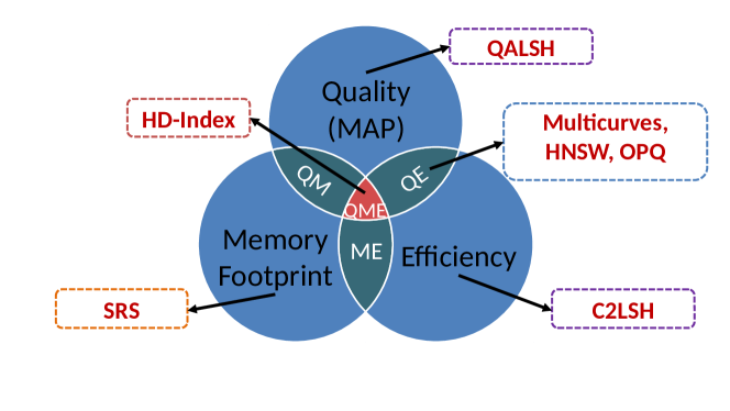
Figure 9: Summarizing the spectrum of approximate nearest neighbor search techniques.

In sum, HD-Index (classified as “QME”) stands strong on all the three pillars, and is an effective, efficient and scalable index structure which scales gracefully to massive high-dimensional datasets even on commodity hardware.

6 Conclusions and Future Work

In this paper, we addressed the problem of approximate nearest neighbor searching in massive high-dimensional datasets within practical compute times while simultaneously exhibiting high quality. We designed an efficient indexing scheme, HD-Index, based on a novel index structure, RDB-tree. Experiments portrayed the effectiveness, efficiency and scalability of HD-Index.

In future, we would like to attempt a parallel implementation to cater to higher dimensional datasets. Also, we would like to analyze the effect of parameters from a theoretical point of view.

Appendix A Reference Object Selection

The comparison of different reference object selection methods is shown in Fig. 10. The method selected is SSS.

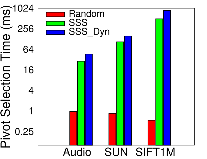
(a) Time

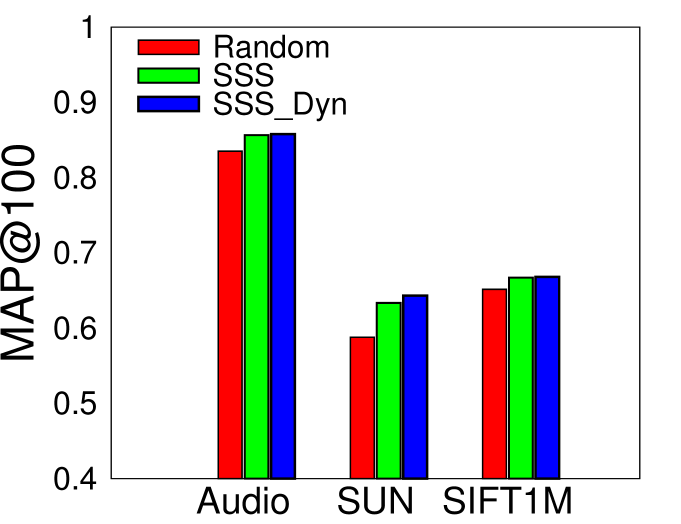
(b) MAP@k

Figure 10: Comparison of different reference object selection algorithms.

Appendix B Ptolemaic Inequality

Fig. 11 and Fig. 12 describe the detailed results of using the triangular inequality alone versus a combination of triangular and Ptolemaic inequalities. For a fixed value of $\alpha$ and the same amount of reduction through the filtering process, using only the triangular inequality provides the fastest response times, being $1.5$-$2$ times faster than when both the inequalities are used. However, it is clear from the highlighted entries in the 5${}^{\text{th}}$ column that usually the best MAP@10 is obtained when the Ptolemaic inequality is employed either alone or in conjunction with the triangular inequality. Since Ptolemaic inequality provides tighter bounds, the improvements in MAP values are prominent where the amount of reduction using the filters is large.

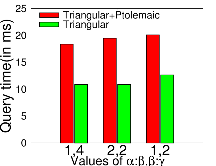
(a) Query Time (SIFT10K)

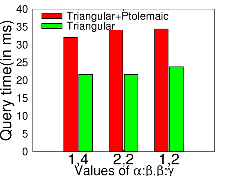
(b) Query Time (AUDIO)

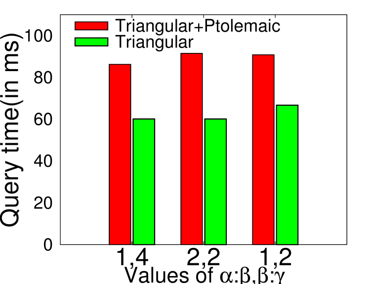
(c) Query Time (SUN)

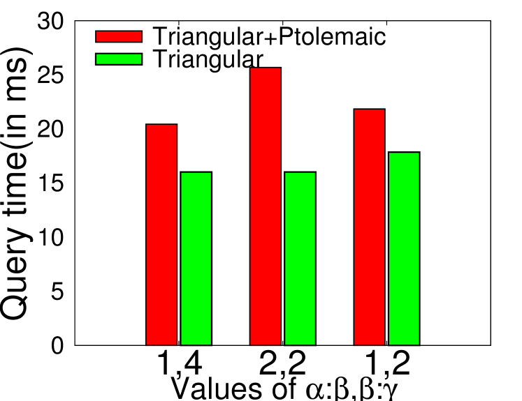
(d) Query Time (SIFT1M)

(e) MAP@10 (SIFT10K)

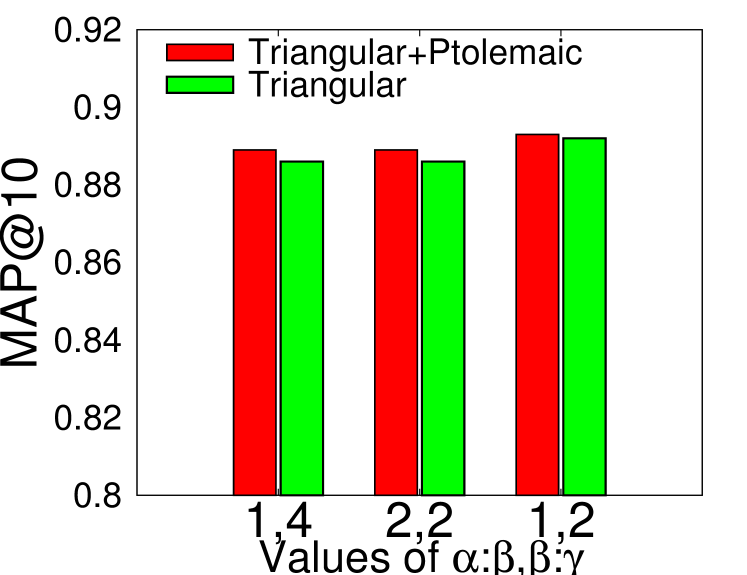
(f) MAP@10 (AUDIO)

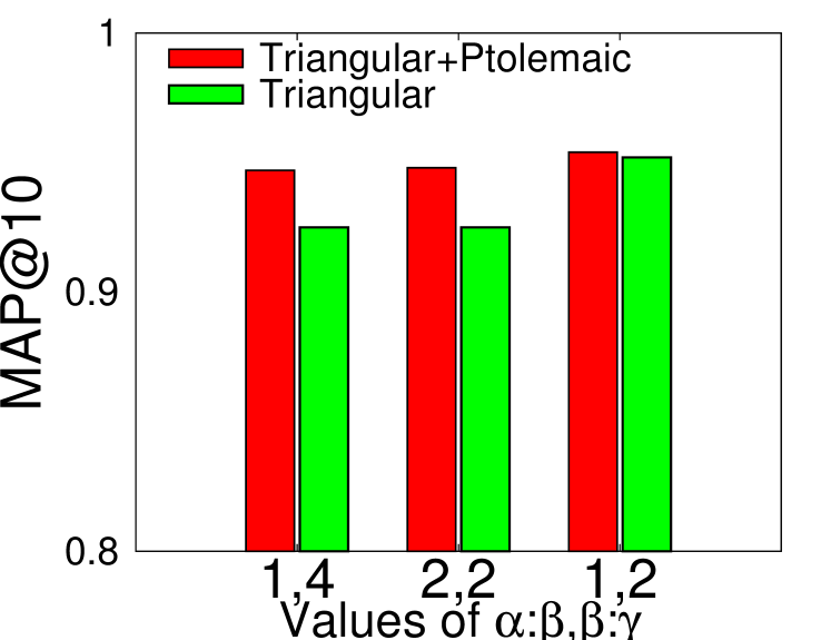
(g) MAP@10 (SUN)

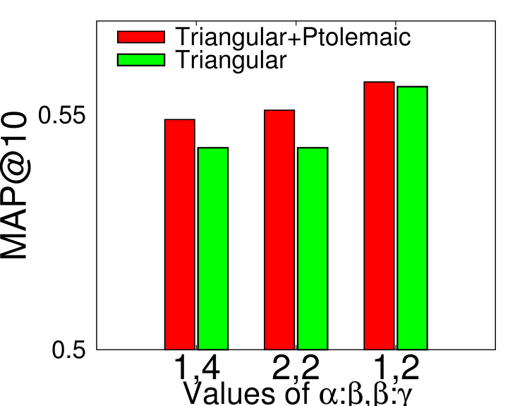
(h) MAP@10 (SIFT1M)

Figure 11: Effect of the filtering mechanism (either triangular inequality alone or a combination of triangular and Ptolemaic inequalities) on query time (a-d) and MAP@10 (e-h) with $\alpha=2048$.

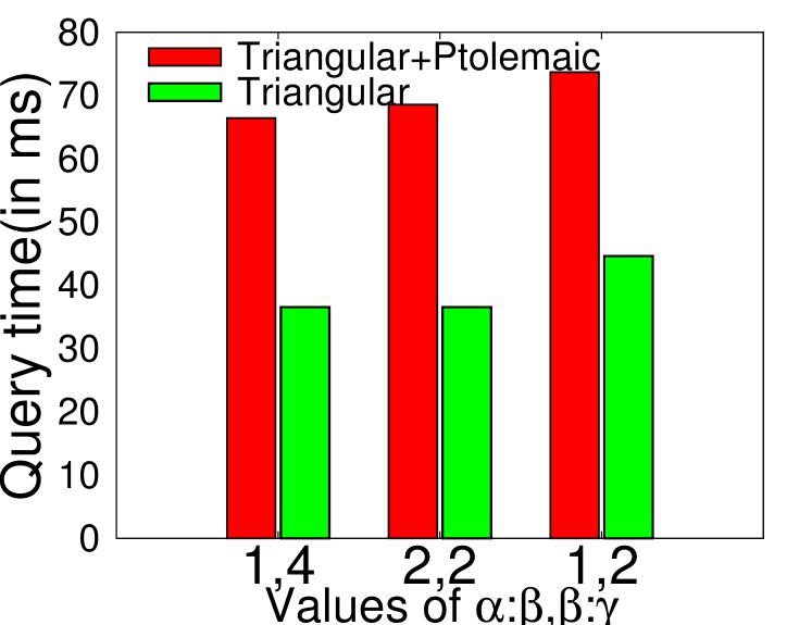
(a) Query Time (SIFT10K)

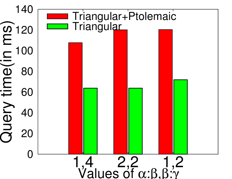
(b) Query Time (AUDIO)

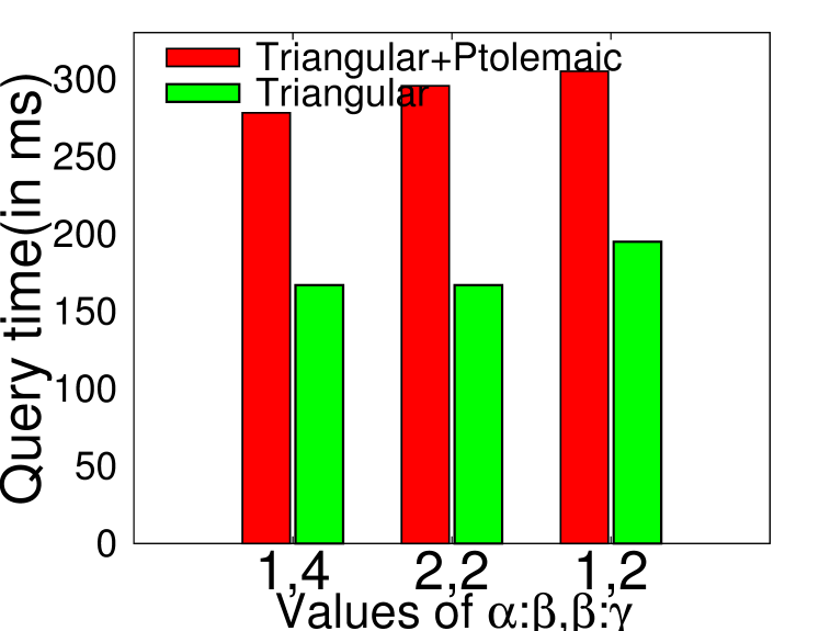
(c) Query Time (SUN)

(d) Query Time (SIFT1M)

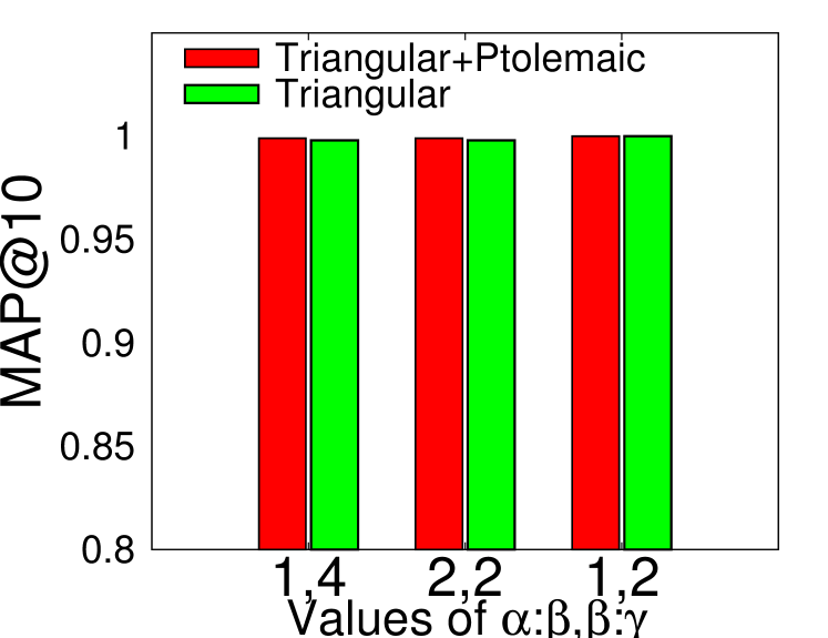
(e) MAP@10 (SIFT10K)

(f) MAP@10 (AUDIO)

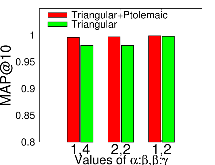
(g) MAP@10 (SUN)

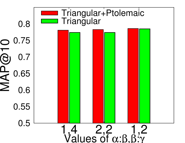
(h) MAP@10 (SIFT1M)

Figure 12: Effect of the filtering mechanism (either triangular inequality alone or a combination of triangular and Ptolemaic inequalities) on query time (a-d) and MAP@10 (e-h) with $\alpha=8192$.

Appendix C Number of Nearest Neighbors

The results of varying the number of nearest neighbors, $k$, for all the methods on the tiny, small and medium datasets are shown in Fig. 13. Since iDistance is an exact method, it always returns correct answers and, hence, possesses a MAP@k of $1$. Consequently, we do not show its MAP results. Moreover, the results of the Multicurves technique is not shown for SUN (Figs. 13c and 13h) due to reasons explained in Sec. 5.4.

The running time remains almost constant for HD-Index and Multicurves, while for the other techniques, it increase with $k$. This is mainly due to the design of HD-Index and Multicurves as explained in Sec. 5.2.7.

Moreover, as shown in Figs. 13a to 13e, even the MAP@k for HD-Index and Multicurves almost remain constant with varying $k$. For the other techniques, MAP@k is unstable with varying $k$. This is due to the fact that when these techniques are allowed to examine more objects, i.e., $k$ is increased, some actual answers are sometimes retrieved. Since the answers are returned in a sorted manner, the true answers find their correct places and MAP increases.

Overall, HD-Index reports the best MAP@$k$ and scales gracefully with dataset size.

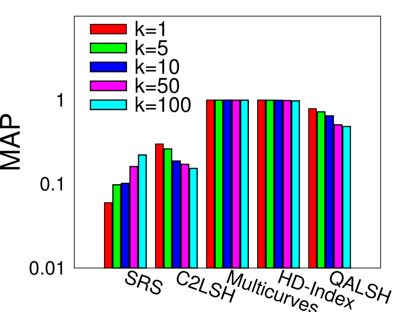
(a) SIFT10K

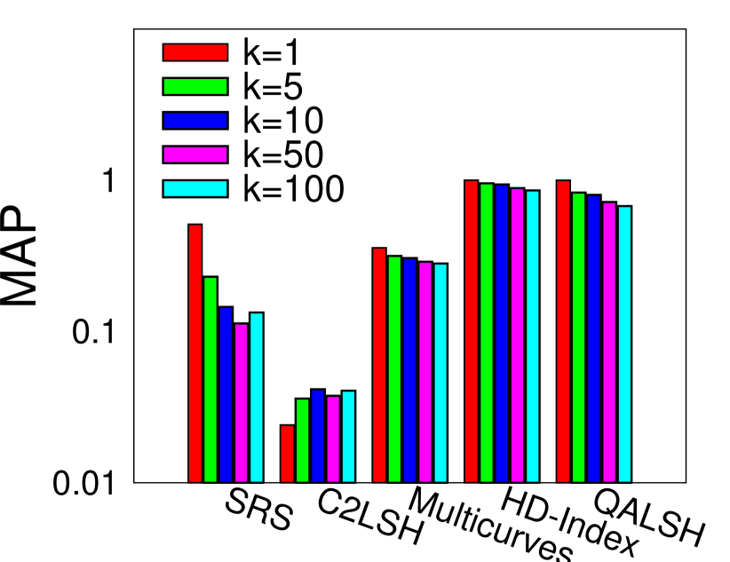
(b) Audio

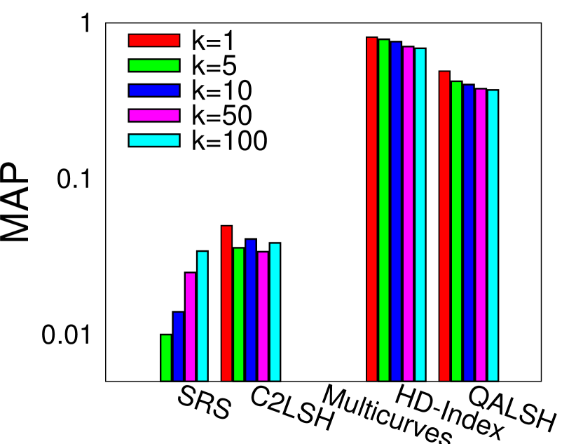
(c) SUN

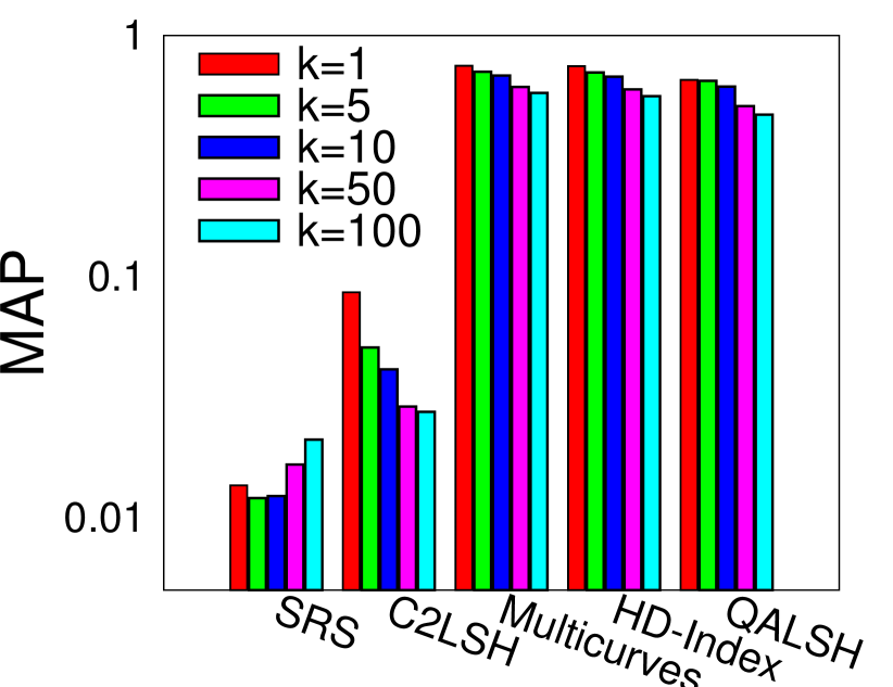
(d) SIFT1M

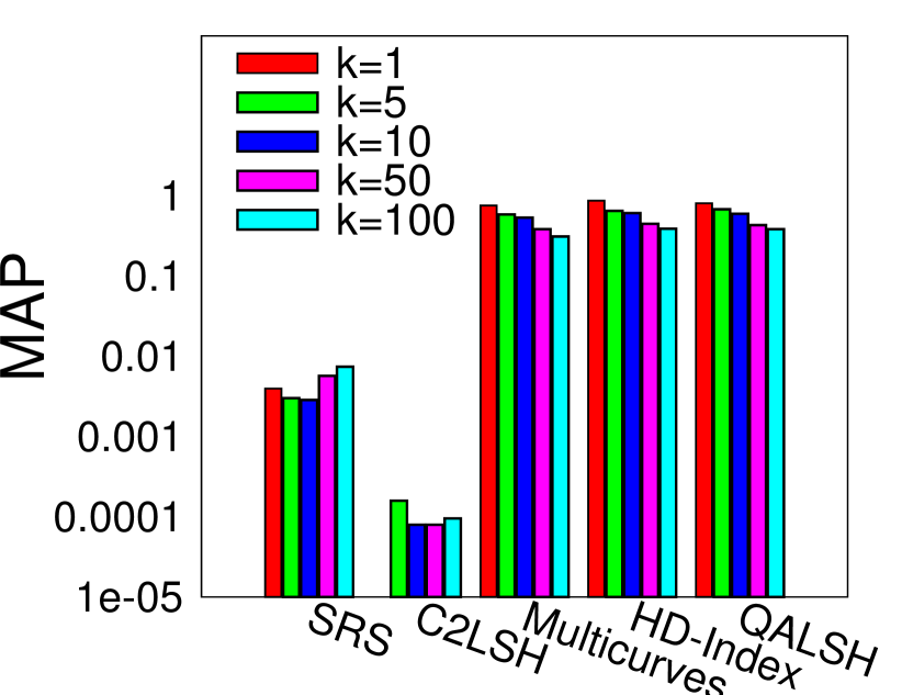
(e) Yorck

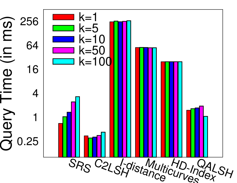
(f) SIFT10K

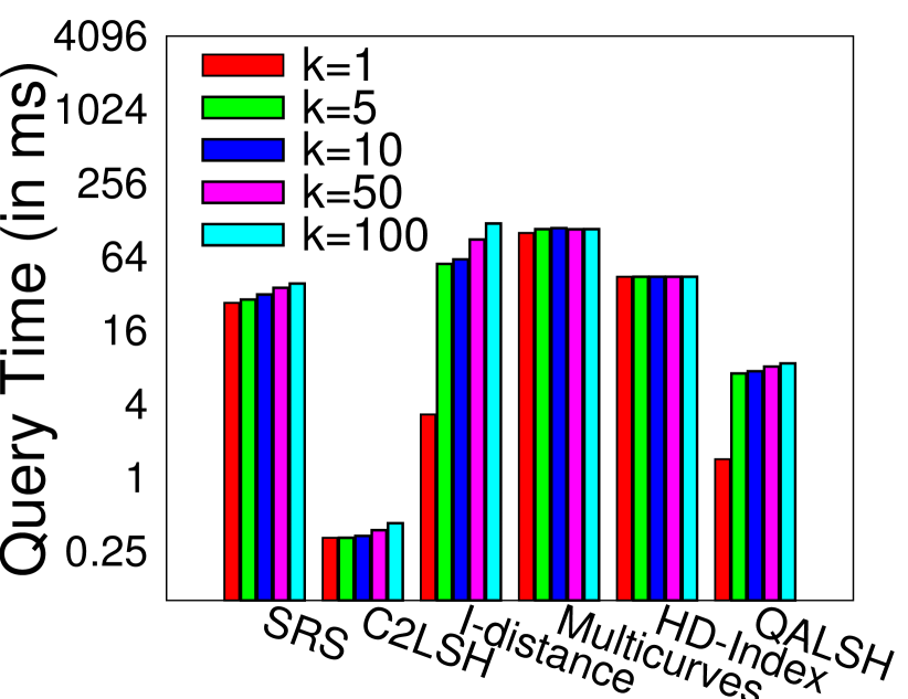
(g) Audio

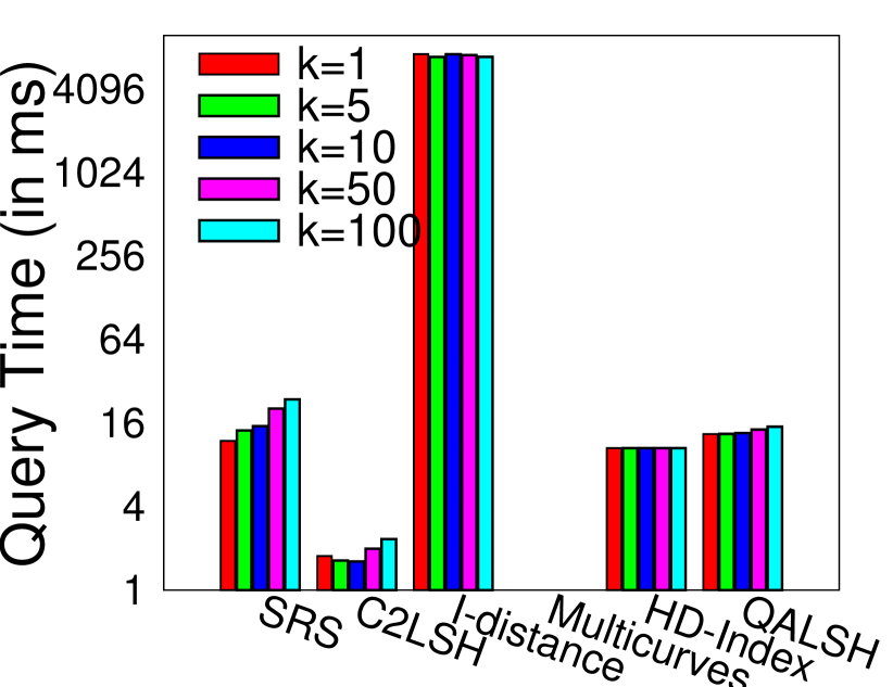
(h) SUN

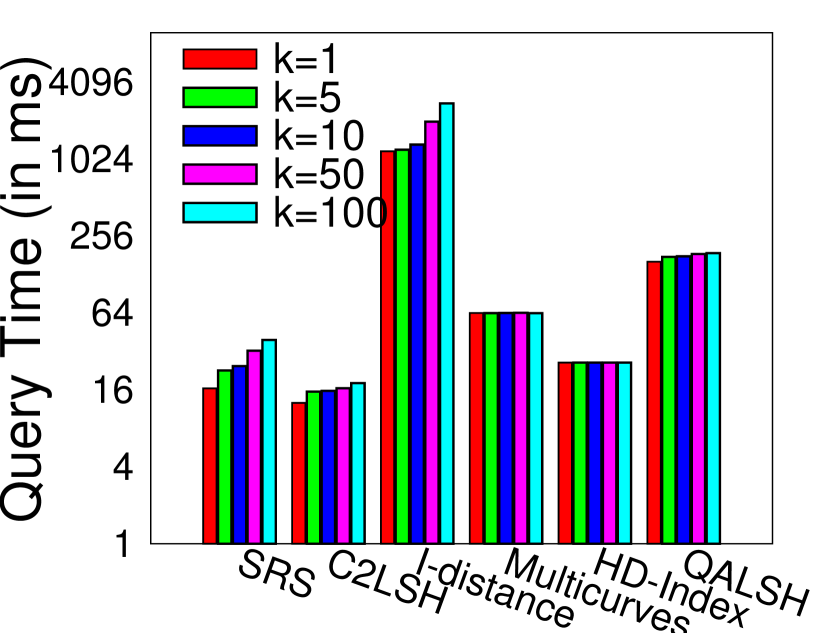
(i) SIFT1M

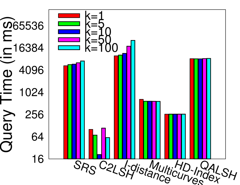
(j) Yorck

Figure 13: Comparison of MAP@$k$ and query time for varying $k$ on different datasets.

Appendix D Borda Count

Consider a query image $q$ with $N$ descriptors. Each descriptor $desc(q)$ is queried against the database and its kANN result set $r(j,q)$ with $|r(j,q)|=k$ descriptors, sorted according to their distance to $desc(q)$ are retrieved. The Borda count method [57] is then employed to get the $k$ nearest neighbor images of $q$.

Consider a database image $i$. A score is given to $i$ based on the depth of its descriptors in the kANN result sets $r(j,q)$ of $q$. For each result set $r(j,q)$, if a descriptor of image $i$ is found at position $l$, then the image $i$ accumulates a score $k+1-l$. These scores are then summed over all the $N$ results sets of $q$ to obtain the Borda count of $i$ against $q$:

$$\text{BC}(i,q)=\sum_{j=1}^{N}\left[\sum_{l=1}^{k}\left((k+1-l).I(i,j,l)\right)\right]$$ (7)

where $I$ is the indicator function that is $1$ only when a descriptor from image $i$ is found at position $l$ of result $r(j,q)$:

$$I(i,j,l)=\begin{cases}1&\text{if descriptor from $i$ occurs at position $l$ of $r(j,q)$}\\ 0&\text{otherwise}\end{cases}$$

The $k$ images with the largest Borda counts are returned in order as the $k$ nearest neighbors of the query image $q$.

Appendix E Image Search Results

The top-$3$ results for a representative query for the different methods is shown in Table 6.

Linear	HD-Index	SRS	C2LSH	Multicurves	QALSH

Table 6: Image search results.

References

- [1] Evaluation of approximate nearest neighbors: Large datasets. http://corpus-texmex.irisa.fr/.
- [2] The CASS Project Repository. http://cs.princeton.edu/cass/audio.tar.gz.
- [3] The Enron Database. http://www.cs.cmu.edu/ enron/.
- [4] The Glove Database. https://nlp.stanford.edu/projects/glove/.
- [5] The SUN Database. http://groups.csail.mit.edu/vision/SUN/.
- [6] The Yorck Project. https://commons.wikimedia.org/wiki/Category:PD-Art_(Yorck_Project).
- [7] G. Amato and P. Savino. Approximate similarity search in metric spaces using inverted files. In ICST, volume 6, pages 1–10, 2008.
- [8] K. Aoyama, K. Saito, H. Sawada, and N. Ueda. Fast approximate similarity search based on degree-reduced neighborhood graphs. In KDD, pages 1055–1063, 2011.
- [9] N. Beckmann, H.-P. Kriegel, R. Schneider, and B. Seeger. The R*-tree: An efficient and robust access method for points and rectangles. In SIGMOD, pages 322–331, 1990.
- [10] S. Berchtold, C. Böhm, H. V. Jagadish, H.-P. Kriegel, and J. Sander. Independent quantization: An index compression technique for high-dimensional data spaces. In ICDE, pages 577–588, 2000.
- [11] S. Berchtold, C. Böhm, and H.-P. Kriegel. The pyramid-technique: towards breaking the curse of dimensionality. In SIGMOD, pages 142–153, 1998.
- [12] S. Berchtold, D. Keim, and H. P. Kriegel. The X-tree: An index structure for high-dimensional data. In VLDB, pages 28–39, 1996.
- [13] A. Beygelzimer, S. Kakade, and J. Langford. Cover trees for nearest neighbor. In ICML, pages 97–104, 2008.
- [14] A. Bhattacharya. Fundamentals of Database Indexing and Searching. CRC Press, 2014.
- [15] C. Böhm, S. Berchtold, and D. A. Keim. Searching in high-dimensional spaces: Index structures for improving the performance of multimedia databases. ACM Comp. Sur. (CSUR), 33(3):322–373, 2001.
- [16] N. R. Brisaboa, A. Farina, O. Pedreira, and N. Reyes. Similarity search using sparse pivots for efficient multimedia information retrieval. In ISM, pages 881–888, 2006.
- [17] B. Bustos, G. Navarro, and E. Chavez. Pivot selection techniques for proximity searching in metric spaces. Patt. Recog. Lett., 24(14):2357–2366, 2003.
- [18] B. Bustos, O. Pedreira, and N. Brisaboa. A dynamic pivot selection technique for similarity search. In SISAP (ICDE Workshops), pages 394–401, 2008.
- [19] A. R. Butz. Alternative algorithm for Hilbert’s space-filling curve. IEEE Trans. Computers, C-20(4):424–426, 1971.
- [20] L. Chen, Y. Gao, X. Li, C. Jensen, and G. Chen. Efficient metric indexing for similarity search. In ICDE, pages 591–602, 2015.
- [21] P. Ciaccia, M. Patella, and P. Zezula. M-tree: An efficient access method for similarity search in metric spaces. In VLDB, pages 426–435, 1997.
- [22] D. Comer. The ubiquitous B-tree. ACM Comp. Sur., 11(2):121–137, 1979.
- [23] S. Dasgupta. Performance guarantees for hierarchical clustering. J. Comput. Syst. Sci., 70(4):555–569, 2005.
- [24] M. Datar, N. Immorlica, P. Indyk, and V. S. Mirrokni. Locality-sensitive hashing scheme based on p-stable distributions. In SCG, pages 253–262, 2004.
- [25] R. Fagin, R. Kumar, and D. Sivakumar. Efficient similarity search and classification via rank aggregation. In SIGMOD, pages 301–312. ACM, 2003.
- [26] J. Gan, J. Feng, Q. Fang, and W. Ng. Locality-sensitive hashing scheme based on dynamic collision counting. In SIGMOD, pages 541–552, 2012.
- [27] T. Ge, K. He, Q. Ke, and J. Sun. Optimized product quantization for approximate nearest neighbor search. In CVPR, pages 2946–2953, 2013.
- [28] A. Guttman. R-trees: A dynamic index structure for spatial searching. In SIGMOD, pages 47–57, 1984.
- [29] C. Hennig and L. J. Latecki. The choice of vantage objects for image retrieval. Pattern Recognition, 36(9):2187–2196, 2003.
- [30] M. L. Hetland, T. Skopal, J. Lokoc, and C. Beecks. Ptolemaic access methods: Challenging the reign of the metric space model. Inf. Syst., 38(7):989–1006, 2013.
- [31] M. E. Houle and M. Nett. Rank-based similarity search: Reducing the dimensional dependence. PAMI, 37(1):136–150, 2015.
- [32] M. E. Houle and J. Sukuma. Fast approximate similarity search in extremely high-dimensional data sets. In ICDE, pages 619–630, 2005.
- [33] Q. Huang, J. Feng, Y. Zhang, Q. Fang, and W. Ng. Query-aware locality-sensitive hashing for approximate nearest neighbor search. PVLDB, 9(1):1–12, 2015.
- [34] P. Indyk and R. Motwani. Approximate nearest neighbors: towards removing the curse of dimensionality. In STOC, pages 604–613, 1998.
- [35] H. Jegou, M. Douze, and C. Schmid. Product quantization for nearest neighbor search. PAMI, 33(1):117–128, 2011.
- [36] C. T. Jr., R. F. S. Filho, A. J. M. Traina, M. R. Vieira, and C. Faloutsos. The Omni-family of all-purpose access methods: A simple and effective way to make similarity search more efficient. VLDB J., 16(4):483–505, 2007.
- [37] I. Kamel and C. Faloutsos. On packing R-trees. In CIKM, pages 490–499, 1993.
- [38] N. Katayama and S. Satoh. The SR-tree: An index structure for high-dimensional nearest neighbor queries. In SIGMOD, pages 369–380, 1997.
- [39] R. Krauthgamer and J. R. Lee. Navigating nets: simple algorithms for proximity search. In SODA, pages 798–807, 2004.
- [40] J. K. Lawder and P. J. H. King. Using space-filling curves for multi-dimensional indexing. In British National Conf. on Databases, pages 20–35, 2000.
- [41] R. H. V. Leuken and R. C. Veltkamp. Selecting vantage objects for similarity indexing. ACM Trans. Mult. Comput., Commun., and Appl., 7(3):16, 2011.
- [42] S. Liao, M. A. Lopez, and S. T. Leutenegger. High dimensional similarity search with space filling curves. In ICDE, pages 615–622, 2001.
- [43] T. Liu, A. W. Moore, A. G. Gray, and K. Yang. An investigation of practical approximate nearest neighbor algorithms. In NIPS, pages 825–832, 2004.
- [44] Y. Liu, J. Cui, Z. Huang, H. Li, and H. T. Shen. SK-LSH: An efficient index structure for approximate nearest neighbor search. PVLDB, 7(9):745–756, 2014.
- [45] Q. Lv, W. Josephson, Z. Wang, M. Charikar, and K. Li. Multi-probe lsh: efficient indexing for high-dimensional similarity search. In VLDB, pages 950–961, 2007.
- [46] G. Mainar-Ruiz and J.-C. Perez-Cortes. Approximate nearest neighbor search using a single space-filling curve and multiple representations of the data points. In ICPR, volume 2, pages 502–505, 2006.
- [47] Y. Malkov, A. Ponomarenko, A. Logvinov, and V. Krylov. Approximate nearest neighbor algorithm based on navigable small world graphs. Information Systems, 45:61–68, 2014.
- [48] Y. A. Malkov and D. A. Yashunin. Efficient and robust approximate nearest neighbor search using hierarchical navigable small world graphs. arXiv:1603.09320 [cs.DS], 2016.
- [49] C. D. Manning, P. Raghavan, and H. Schütze. Introduction to Information Retrieval. Cambridge University Press, 2008.
- [50] M. Marin, V. Gil-Costa, and R. Uribe. Hybrid index for metric space databases. In ICCS, pages 327–336, 2008.
- [51] N. Megiddo and U. Shaft. Efficient nearest neighbor indexing based on a collection of space filling curves. Technical Report IBM Research Report RJ 10093 (91909), IBM Almaden Research Center, San Jose California, 1997.
- [52] M. L. Micó, J. Oncina, and E. Vidal. A new version of the nearest-neighbour approximating and eliminating search algorithm (AESA) with linear preprocessing time and memory requirements. Patt. Recog. Lett., 15(1):9–17, 1994.
- [53] M. Muja and D. G. Lowe. Scalable nearest neighbor algorithms for high dimensional data. Pattern Analysis and Machine Intelligence, IEEE Transactions on, 36, 2014.
- [54] M. Norouzi and D. J. Fleet. Cartesian k-means. In CVPR, pages 3017–3024, 2013.
- [55] B. C. Ooi, K.-L. Tan, C. Yu, and S. Bressan. Indexing the edges – a simple and yet efficient approach to high-dimensional indexing. In PODS, pages 166–174, 2000.
- [56] O. Pedreira and N. R. Brisaboa. Spatial selection of sparse pivots for similarity search in metric spaces. In SOFSEM (1), pages 434–445, 2007.
- [57] B. Reilly. Social choice in the south seas: Electoral innovation and the borda count in the pacific island countries. Int. Political Sc. Rev., 23, 2002.
- [58] E. V. Ruiz. An algorithm for finding nearest neighbors in (approximately) constant average time. Patt. Recogn. Lett., 4(3):145–157, 1986.
- [59] H. Sagan. Space-Filling Curves. Springer, 1994.
- [60] Y. Sakurai, M. Yoshikawa, S. Uemura, and H. Kojima. The A-tree: An index structure for high-dimensional spaces using relative approximation. In VLDB, pages 516–526, 2000.
- [61] H. Samet. Foundations of Multidimensional and Metric Data Structures. Morgan Kaufmann, 2005.
- [62] J. Shepherd, X. Zhu, and N. Megiddo. A fast indexing method for multidimensional nearest neighbor search. In SPIE, pages 350–355, 1999.
- [63] C. Silpa-Anan and R. Hartley. Optimised kd-trees for fast image descriptor matching. In CVPR, pages 1–8, 2008.
- [64] Y. Sun, W. Wang, J. Qin, Y. Zhang, and X. Lin. SRS: Solving c-approximate nearest neighbor queries in high dimensional Euclidean space with a tiny index. PVLDB, 8(1):1–12, 2014.
- [65] Y. Tao, K. Yi, C. Sheng, and P. Kalnis. Quality and efficiency in high dimensional nearest neighbor search. In SIGMOD, pages 563–576, 2009.
- [66] E. Valle, M. Cord, and S. Philipp-Foliguet. High-dimensional descriptor indexing for large multimedia databases. In CIKM, pages 739–748, 2008.
- [67] J. Venkateswaran, T. Kahveci, C. M. Jermaine, and D. Lachwani. Reference-based indexing for metric spaces with costly distance measures. VLDB J., 17(5):1231–1251, 2008.
- [68] E. Vidal. New formulation and improvements of the nearest-neighbour approximating and eliminating search algorithm (AESA). Patt. Recogn. Lett., 15(1):1–7, 1994.
- [69] J. Wang and S. Li. Query-driven iterated neighborhood graph search for large scale indexing. In ACM Multimedia, pages 179–188, 2012.
- [70] J. Wang, J. Wang, G. Zeng, R. Gan, S. Li, and B. Guo. Fast neighborhood graph search using Cartesian concatenation. In Multimedia Data Mining and Analytics, pages 397–417, 2015.
- [71] R. Weber, H.-J. Schek, and S. Blott. A quantitative analysis and performance study for similarity-search methods in high-dimensional spaces. In VLDB, pages 194–205, 1998.
- [72] D. A. White and R. Jain. Similarity indexing with the SS-tree. In ICDE, pages 516–523, 1996.
- [73] C. Yu, B. C. Ooi, K.-L. Tan, and H. V. Jagadish. Indexing the distance: An efficient method to knn processing. In VLDB, pages 421–430, 2001.