OSU-HEP-18-02

Displaced vertex signature of type-I seesaw

Sudip Jana^a,b,, Nobuchika Okada^c, and Digesh Raut^c,

^aTheory Department, Fermi National Accelerator Laboratory,
P.O. Box 500, Batavia, IL 60510, USA
^bDepartment of Physics, Oklahoma State University,
Stillwater, OK 74078-3072, USA
^cDepartment of Physics and Astronomy, University of Alabama,
Tuscaloosa, Alabama 35487, USA

A certain class of new physics models includes long-lived particles which are singlet under the Standard Model (SM) gauge group. A displaced vertex is a spectacular signature to probe such particles productions at the high energy colliders, with a negligible SM background. In the context of the minimal gauged $B-L$ extended SM, we consider a pair creation of Majorana right-handed neutrinos (RHNs) at the high energy colliders through the production of the SM and the $B-L$ Higgs bosons and their subsequent decays into RHNs. With parameters reproducing the neutrino oscillation data, we show that the RHNs are long-lived and their displaced vertex signature can be observed at the next generation displaced vertex search experiments, such as the HL-LHC, the MATHUSLA, the LHeC, and the FCC-eh. We find that the lifetime of the RHNs is controlled by the lightest light neutrino mass, which leads to a correlation between the displaced vertex search and the search limit of the future neutrinoless double beta-decay experiments.

1 Introduction

The last missing piece of the Standard Model (SM) is finally supplemented with the discovery of the Higgs boson at the Large Hadron Collider (LHC) in 2012 [1, 2], which itself is not that surprising given the tremendous success of the SM to explain observed elementary particle phenomena. However, the SM is not complete in its current form, because, for example, the neutrinos are massless in the framework which is not consistent with the experimental evidence of the neutrino oscillation phenomena [3], indicating that the neutrinos have tiny non-zero masses and flavor mixings. Hence, we need to extend the current framework of the SM.

Unfortunately, ever since the discovery of the SM Higgs boson, no new signature of new physics beyond the SM has been observed. It may indicate that the current energy and luminosity of the LHC are not sufficient to directly probe new particles. If so, we can just hope for new particle signals to be observed at the future LHC after the planned upgrade, or at a future collider with energies higher than the LHC. However, there is another possibility: if new particles are completely singlet under the SM gauge group, it can naturally explain the null search results at the LHC because SM singlet particles cannot be directly produced at the LHC through the SM interactions. Such particles may be produced through new interactions and/or rare decay of the SM particles. At a first glance, it seems that such a scenario is even more challenging to test. However, if a new particle is long-lived, it can leave a displaced vertex signature at the collider experiments. Since the displaced vertex signatures are generally very clean, they allow us to search for such a particle with only a few events at the LHC or future colliders. For the current status of displaced vertex searches at the LHC, see, for example, Refs. [4, 5, 6, 7, 8, 9, 10, 11, 12, 13, 14, 15, 16, 17, 18, 19, 20, 21]. The search reach will be dramatically improved in the future planned/proposed experiments, such as the High-Luminosity LHC (HL-LHC), the MATHUSLA [22], the Large Hadron electron Collider (LHeC)[23] and the the Future Circular electron-hadron Colliders (FCC-eh) [24].

In this paper, we first review the current theoretical and experimental studies focusing on the displaced vertex searches at the future collider experiments and express their results in a model independent form. As a concrete example, we consider a well-motivated simple extension of the SM, namely the minimal $B-L$ (baryon minus lepton number) model [25, 26, 27, 28, 29, 30], where the global ${B-L}$ symmetry in the SM is promoted to the gauge symmetry. A minimal $B-L$ model includes an additional electrically neutral gauge boson ($Z^{\prime}$ boson) as well as a $B-L$ Higgs boson which breaks the ${B-L}$ symmetry. In addition, the model also includes three right-handed neutrinos (RHNs) to cancel all the gauge and mixed-gravitational anomalies. After the $B-L$ symmetry breaking, the RHNs acquire Majorana masses, and the tiny neutrinos masses are automatically generated through the so-called type-I seesaw mechanism [31, 32, 33, 34, 35, 36] after the electro-weak symmetry breaking. In this model context, we investigate the displaced vertex signature of the Majorana RHNs at the future high energy colliders through the production of the SM and the $B-L$ Higgs bosons and their subsequent decays into RHNs. Since the Majorana RHNs decay into the SM particles through small light-heavy neutrino mixings from type-I seesaw, the RHNs are likely to be long-lived.

This paper is organized as follows. In Sec. 2, we review the prospect of the search reach of displaced vertex signatures at the future high energy colliders. Employing the (2$\sigma$) search reach of the displaced vertex signatures obtained in various analysis, we present a model-independent formula for the search reach in terms of the production cross section of a long-lived particle as a function of its lifetime, mass and its mother particle mass whose decay products are the long-lived particle. In Sec. 3, we give a review on the minimal $B-L$ extended SM. In Sec. 4, we consider the pair production of RHNs through the production of the Higgs bosons and their subsequent decays into RHNs. We apply the best reach values for the production cross section obtained in Sec. 2 to the RHNs production, assuming a suitable lifetime of the RHNs. For benchmark mass values of the $B-L$ Higgs boson and RHNs, we determine the corresponding parameter space for RHNs Majorana Yukawa couplings and a mixing between the SM and the $B-L$ Higgs bosons. In Sec. 5, we calculate the lifetime of the RHNs for realistic parameters to reproduce the neutrino oscillation data. Using this realistic value for the lifetime, we repeat the analysis in Sec. 4 to determine the parameter space corresponding to the search reach. In Sec. 6 we discuss the correlation between the displaced vertex search and the search limit of the future neutrinoless double beta-decay experiments. Sec. 7 is devoted to conclusions.

2 Displaced vertex search at the future colliders

An electrically neutral particle with a sufficiently long lifetime (for example, its decay length is of $\mathcal{O}$(1 mm) or larger), once produced at the colliders, displays a signature of the displaced vertex, namely the vertex created by the decay of the particles is located away from the collision point where the particle is produced. The final state charged leptons and/or jets from a displaced vertex can be reconstructed by a dedicated displaced vertex analysis. Since displaced vertex signatures from SM particles are very well understood, the signature from a new long-lived particle can be easily distinguished, making it a powerful probe to discover such particles.

Let us first review the search reach of displaced vertex signatures at the future colliders which have been investigated in Refs. [22, 56, 57]. In Refs. [22, 56], the authors have proposed the MATHUSLA detector which is specifically designed to explore the long lifetime frontier; the plan is to build a detector on the ground, about 100 m away from the HL-LHC detector. The authors have also considered displaced vertex using the inner-detector of the HL-LHC. Similarly, in the Ref. [57], the authors have studied the prospect of a dedicated displaced vertex search at the future electron-proton colliders, such as the LHeC and the FCC-eh. In their analysis, they consider a pair production of a long-lived particle “X" created from the rare decay of the SM Higgs boson. They have shown the search reach for the branching ratio of the SM Higgs boson to a pair of X particles as a function of X particle’s decay length ($c\tau$) ranging from sub-millimeter to $10^{7}$ m.

Figure 1: The plot shows the discovery reach for a dedicated displaced vertex searches at the future experiments and newly proposed extensions to the current LHC experiment. The lines corresponds to the total production cross section to produce a pair of “X” particles in the final states as a function of the X particle decay length, where the mass of the X particle and its mother-particle are fixed to be 20 GeV and 125 GeV, respectively. The region above the dashed (solid) line corresponds to the search reach at the HL-LHC and the MATHUSLA experiements. The dotted curved lines correspond to the search reach of the various proposed electron-proton collider upgrade of HL-LHC.

We first summarize the results in Refs. [22, 56, 57] in Fig. 1. Here, for a fixed mass of the X particle ($m_{X}=20$ GeV), we show the search reach for the X particle pair production cross section ($\sigma_{XX}$) at the future colliders as a function of the lifetime of X particle $c\tau$. The dashed and solid lines show the search reach for the displaced vertex signatures at the HL-LHC and the MATHUSLA experiments, respectively, with a 3 ab^-1 luminosity. The dotted lines (almost degenerate) correspond to the discovery reach at the FCC-eh with a 3 ab^-1 with electron beam energies of 60 GeV (top) and the LHeC with a 1 ab^-1 (bottom).

Figure 2: The search reach of the displaced vertex signatures at the HL-LHC (dashed lines in Fig. 1) for $m_{S}=50$ (solid), $125$ (dashed) and $400$ (dot-dashed) GeV with $m_{X}=20$ GeV. We have employed Eq. (2.2) to plot the lines for $m_{S}=50$ and $400$ GeV, based on the dashed line for $m_{S}=125$ GeV.

In Fig. 1, the process $pp/ep\to h\to XX$ is considered. We generalize the process to $pp/ep\to S\to XX$, where the mother-particle ($S$) is a boson, but not the SM Higgs boson, with a mass $m_{S}$. In order to make the results in Fig. 1 to applicable to this general case, note that the search reach shown in Fig. 1 is model-independent if the curves are plotted as a function of the lifetime of X in the laboratory frame. For the process $pp/ep\to h\to XX$, the lifetime of the particle X in the laboratory frame ($\tau^{\prime}$) is given by its proper lifetime ($\tau$) as

$$\tau^{\prime}=\left(\frac{m_{h}}{2m_{X}}\right)\tau,$$ (2.1)

because of the Lorentz boost. We then express the search reach of the cross sections in Fig. 1 as $\sigma_{XX}(c\tau)=\sigma_{XX}\left(\frac{2m_{X}}{m_{h}}c\tau^{\prime}\right)$. The model-independent search reach can be obtained as a function of $c\tau^{\prime}$ for the fixed values of $m_{h}=125$ GeV and $m_{X}=20$ GeV. Now it is easy to convert the search reach results in Fig. 1 to our general case:

$$\sigma(pp/ep\to S\to XX)=\sigma_{XX}\left(c\tau\times\frac{m_{S}}{125\,{\rm GeV}}\times\frac{20\,{\rm GeV}}{m_{X}}\right),$$ (2.2)

where $\sigma_{XX}(c\tau)$ represents different curves shown in Fig. 1. Hence, depending on the choice of masses for $m_{S}$ and $m_{X}$, the curves shown in Fig. 1 shifts either to the left or to the right. In Ref. [56], the search reach of the cross sections are shown for three benchmark values of $m_{X}=5$, $20$ and $40$ GeV. We have checked that our formula of Eq. (2.2) can reproduce the results for $m_{X}=5$ and $40$ GeV in Ref. [56] from the result for $m_{X}=20$ GeV. In Fig. 2, we show the search reach at the HL-LHC for $m_{S}=50$ GeV (solid line) and $m_{S}=400$ GeV (dot-dashed line) by employing the result for $m_{S}=125$ GeV (dashed line) and Eq. (2.2). Here, we have fixed $m_{X}=20$ GeV. As we raise/lower $m_{S}$ for $m_{X}=20$ GeV, the line shifts to the left/right, since the created X particle is more/less boosted. In the following, we employ the generalized formula to investigate the search reach of long-lived RHNs at the future high energy colliders.

3 The minimal $B-L$ extended Standard Model

	SU(3)c	SU(2)L	U(1)Y	U(1)B-L
$q_{L}^{i}$	3	2	$+1/6$	$+1/3$
$u_{R}^{i}$	3	1	$+2/3$	$+1/3$
$d_{R}^{i}$	3	1	$-1/3$	$+1/3$
$\ell^{i}_{L}$	1	2	$-1/2$	$-1$
$N_{R}^{i}$	1	1	$0$	$-1$
$e_{R}^{i}$	1	1	$-1$	$-1$
$H$	1	2	$-1/2$	$0$
$\varphi$	1	1	$0$	$+2$

Table 1: Particle content of the minimal $B-L$ model. In addition to the SM particle content, three RHNs ($N_{R}^{i}$, $i=1,2,3$ denotes the generation index) and a complex scalar ($\varphi$) are introduced.

Here we review the minimal $B-L$ extended SM (the minimal $B-L$ model). The particle content of the model is listed in Table 1. In this model, the global $B-L$ symmetry in the SM is gauged, and in addition to the SM particle content, three RHNs and a complex scalar ($B-L$ Higgs field) are introduced. While the $B-L$ Higgs field spontaneously breaks the $B-L$ symmetry by its vacuum expectation value (VEV), the three RHNs are necessary to cancel all the gauge and mixed-gravitational anomalies.

The Yukawa sector of the SM is extended to include

$$\mathcal{L}_{Y}\supset-\sum_{i,j=1}^{3}Y_{D}^{ij}\overline{\ell_{L}^{i}}HN_{R}^{j}-\frac{1}{2}\sum_{k=1}^{3}Y_{N}^{k}\Phi\overline{N_{R}^{k\ c}}N_{R}^{k}+\rm{h.c.},$$ (3.1)

where the first and second terms are the Dirac and Majorana Yukawa couplings. Here, we work on a diagonal basis for the Majorana Yukawa couplings ($Y_{N}$) without loss of generality. Associated with the $B-L$ gauge symmetry breaking, the $B-L$ gauge boson ($Z^{\prime}$ boson) and the RHNs acquire their masses as follows:

$$m_{Z^{\prime}}=2\,g\,v_{BL},\;\;m_{N^{i}}=\frac{Y_{N}^{i}}{\sqrt{2}}v_{\Phi},$$ (3.2)

where $v_{BL}=\sqrt{2}\langle\varphi\rangle$ is the VEV of the $B-L$ Higgs field.

A renormalizable scalar potential for the $B-L$ Higgs field ($\varphi$) and the SM Higgs doublet ($H$) is given by

$$V(|H|,|\varphi|)=\lambda\left(|\varphi|^{2}-\frac{v^{2}_{BL}}{2}\right)^{2}+\lambda_{H}\left(|H|^{2}-\frac{v^{2}_{SM}}{2}\right)^{2}+\lambda^{\prime}\left(|H|^{2}-\frac{v^{2}_{SM}}{2}\right)\left(|\varphi|^{2}-\frac{v^{2}_{BL}}{2}\right),$$ (3.3)

where $v_{SM}=246$ GeV is the VEV of the SM Higgs doublet, and we take $\lambda^{\prime}>0$ which introduces a mixing between the two scalar fields. In the unitary gauge, we expand the SM and $B-L$ Higgs fields around their VEVs, $\langle H\rangle=(\frac{v_{SM}}{\sqrt{2}}\;\;0)^{T}$ and $\langle\varphi\rangle=v_{BL}/\sqrt{2}$, to identify $\phi_{SM}$ and $\phi_{BL}$ being the SM and the $B-L$ Higgs bosons in the original basis. The mass matrix for the Higgs bosons is given by

$${\cal L}\supset-\frac{1}{2}\begin{bmatrix}\phi_{SM}&\phi_{BL}\end{bmatrix}\begin{bmatrix}m_{H}^{2}&\lambda^{\prime}v_{BL}v_{SM}\\ \lambda^{\prime}v_{BL}v_{SM}&m_{\varphi}^{2}\end{bmatrix}\begin{bmatrix}\phi_{SM}\\ \phi_{BL}\end{bmatrix},$$ (3.4)

where $m_{H}=\sqrt{2\lambda_{H}}v_{{SM}}$, and $m_{\varphi}^{2}=2\lambda v_{BL}^{2}$. We diagonalize the mass matrix by

$$\begin{bmatrix}\phi_{SM}\\ \phi_{BL}\end{bmatrix}=\begin{bmatrix}\cos\theta&\sin\theta\\ -\sin\theta&\cos\theta\end{bmatrix}\begin{bmatrix}h\\ \phi\end{bmatrix},$$ (3.5)

where $h$ and $\phi$ are the mass eigenstates. The relations among the mass parameters and the mixing angle ($\theta$) are the following:

$$2v_{BL}v_{{SM}}\lambda^{\prime}=(m_{H}^{2}-m_{\varphi}^{2})\tan 2\theta,$$

$$m_{h}^{2}=m_{H}^{2}-\left(m_{\varphi}^{2}-m_{H}^{2}\right)\frac{\sin^{2}\theta}{1-2\sin^{2}\theta},$$

$$m_{\phi}^{2}=m_{\varphi}^{2}+\left(m_{\varphi}^{2}-m_{H}^{2}\right)\frac{\sin^{2}\theta}{1-2\sin^{2}\theta}\ .$$ (3.6)

The properties of the Higgs boson measured at the LHC are consistent with the SM predictions, so that the mixing angle $\theta$ must be small. In this case, we identify the mass eigenstates $h\simeq\phi_{SM}$ and $\phi\simeq\phi_{BL}$ as mostly the SM and $B-L$ Higgs bosons with masses $m_{h}\simeq m_{H}$ and $m_{\varphi}\simeq m_{\phi}$, respectively. We set $m_{H}=125$ GeV in the following. For completeness, we show in Fig. 3 the relation between $m_{\varphi}$ and $\sin\theta$ for a fixed $v_{\varphi}=200$ GeV and various values of $\lambda^{\prime}$. As can be understood from the first line in Eq. (3.6), $m_{H}=m_{\phi}$ is a singular point where the mixing becomes large.

Figure 3: The mixing angle as a function of $m_{\varphi}$ for $v_{BL}=200$ GeV and various values of $\lambda^{\prime}$. The solid lines from top to bottom corresponds to $\lambda^{\prime}=10^{-1},10^{-1},10^{-2},10^{-3}$, and $10^{-4}$.

4 Displaced vertex signature of heavy neutrinos

Let us now consider the displaced vertex signatures of the heavy neutrinos $N^{i}$ in the minimal $B-L$ model.. For the main process for a pair production of $N_{i}$, we can consider two cases: one is through the $Z^{\prime}$ boson production [(see, forexample, Ref.~\cite[cite]{[\@@bibref{}{}{}{}]})] and its decay to $N_{i}$s, and the other is through the production of the Higgs bosons ($h$ and $\phi$) and their decays. The LHC results on the search for the $Z^{\prime}$ boson resonance of the minimal $B-L$ model severely constrain the $B-L$ gauge coupling to be very small (see, for example, Ref. [62]), so that the heavy neutrino production cross section from the $Z^{\prime}$ boson decay is expected to be small. Hence, we focus on the heavy neutrino production through the Higgs bosons in this paper.

Because of its representation under the gauge groups, $\phi_{BL}$ has no tree level coupling with the SM particles at the renormalizable level, and hence it cannot be directly produced at the high colliders. However, as described in Eqs. (3.5) and (3.6), the mass eigenstates are mixture of $\phi_{BL}$ and $\phi_{SM}$ and through the mixing, the Higgs boson $\phi$ can be produced through the same process as the SM Higgs boson. At the LHC, among a variety of the production processes of the SM Higgs boson, such as gluon-gluon fusion (ggF), vector boson fusion (VBF), and the productions associated with $W/Z$ bosons ($Vh$) and with $t\bar{t}$ ($t\bar{t}h$), the ggF channel dominates the production cross section. For a small mixing, the production cross section of the SM-like Higgs boson ($h$) is given by

$$\sigma(pp\to h)=\cos^{2}\theta\times\sigma_{h}(m_{h}),$$ (4.1)

where $\sigma_{h}(m_{h})$ is the SM Higgs boson production cross section with the Higgs boson mass of $m_{h}=125$ GeV. In the limit of $\theta\to 0$, $\sigma(pp\to h)$ reduces to the SM case. Similarly, the production cross section for the $B-L$-like Higgs boson ($\phi$) is expressed as

$$\sigma(pp\to\phi)=\sin^{2}\theta\times\sigma_{h}(m_{\phi}),$$ (4.2)

where $\sigma_{h}(m_{\phi})$ is the SM Higgs boson production cross section if the Higgs boson mass were $m_{\phi}$ As discussed before, we are interested in a small mixing, and hence for the remainder of this paper, we shall simply refer to the mass eigenstates $h$ and $\phi$ as the SM(-like) Higgs boson and the $B-L$ Higgs, respectively.

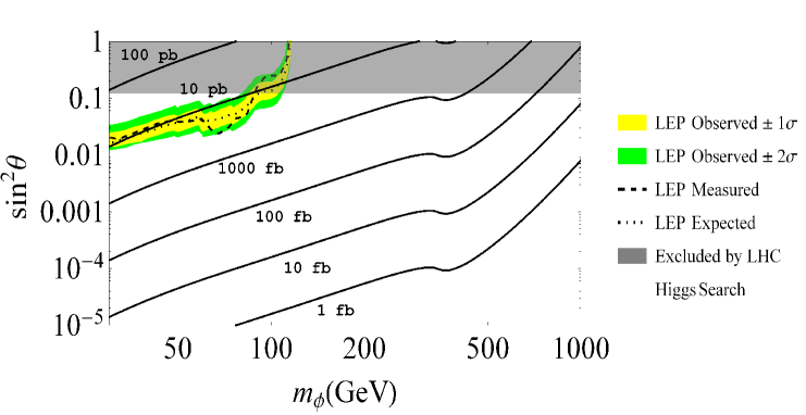
Figure 4: The $B-L$ Higgs production cross section at the 13 TeV LHC in $(m_{\phi},\sin^{2}\theta)$-plane, along with the upper bounds on $\sin^{2}\theta$ from the LEP and the LHC experiments. The region above the dashed curve is excluded by the LEP experiments, while the gray shaded region is excluded by the LHC experiments.

Using Eq. (4.2), we show in Fig. 4 the contour plot for the production cross section of $\phi$ at the 13 TeV LHC ($\sigma(pp\to\phi)$) in the ($m_{\phi},\sin^{2}\theta$)-plane. Here, we also show the constraint obtained by the LEP experiments on the search for the SM Higgs boson through its production associated with the $Z$ boson [65]. For a given Higgs boson mass, no evidence of the SM Higgs boson production sets an upper bound on the $Z$-boson associate production cross section, which is interpreted to be an upper bound on the anomalous SM Higgs coupling with $Z$ boson as a function of the Higgs boson mass. In our model, this upper bound is interpreted as an upper bound on $\sin\theta$ as a function of $m_{\phi}$, which is shown as the dashed curve in Fig. 4. The gray shaded region in the figure is excluded by the current measurement of the SM Higgs boson properties by the ATLAS and CMS collaborations. The Higgs boson properties are characterized by the signal strengths defined as

$$\mu^{i}_{f}=\frac{\sigma^{i}\cdot BR_{f}}{(\sigma^{i})_{SM}\cdot(BR_{f})_{SM}}=\mu^{i}\cdot\mu_{f},$$ (4.3)

where $\sigma^{i}$ are the Higgs boson production cross sections through $i$-channel with $i=ggF,VBF,$ $Wh,$ $Zh,$ $t\bar{t}h$, and $BR_{f}$ are the Higgs boson branching ratios into final states $f=ZZ^{\star},$ $WW^{\star},$ $\gamma\gamma,$ $\tau^{+}\tau^{-},$ $b\bar{b},$ $\mu^{+}\mu^{-}$. The cross sections and branching ratios with the subscript “$SM$” denote the SM predictions. The latest updates of the signal strengths from the ATLAS and the CMS experiments at the LHC Run II with a $37$ fb^-1 luminosity are listed in Refs. [66, 64], along with the references. The averaged signal strength is obtained as $\mu\simeq 0.925\pm 0.134$, which is consistent with the SM prediction $\mu=1$. In our model, the couplings of the SM-like Higgs boson is modified by a factor $\cos\theta$ from the SM case. Hence, the production cross section of $h$ is scaled by $\cos^{2}\theta$ while its branching ratios remain the same as the SM one. Therefore, the signal strengths are given by $\mu^{i}_{f}=\cos^{2}{\theta}\times\mu_{f}$. In anticipation of the analysis presented below, we also consider the constraint from the invisible SM Higgs decay modes, and the current upper bound on the branching ratio of the Higgs invisible decay mode is given by ${BR}_{\rm inv}^{\rm higgs}<0.23$ [67]. Together with the averaged signal strength, we obtain an upper bound on the mixing angle as $\sin^{2}{\theta}\leq 0.12$ at 95$\%$ C.L and the excluded region is depicted by the gray shaded region in Fig.4. Hence, for the entire range of $m_{\phi}$ shown in the figure, the mixing angle is small.

Figure 5: Total decay width of SM Higgs as a function of the Higgs mass.

We now consider the decay of the Higgs bosons. In the presence of the mixing, the total decay width of the SM-like Higgs and the $B-L$ Higgs into the SM final states are given by

$$\Gamma(h\to SM) = \cos^{2}\theta\times\Gamma_{SM}(m_{h}),$$

$$\Gamma(\phi\to SM) = \sin^{2}\theta\times\Gamma_{{SM}}(m_{\phi}),$$ (4.4)

respectively, where $\Gamma_{SM}(M)$ is the total decay width of the SM Higgs boson if the SM Higgs mass were $M$. The list of the partial decay widths of the SM-like Higgs boson is given in the Appendix. In Fig. 5 we show the total decay width $\Gamma_{SM}(m_{H})$ as a function $m_{H}$. The partial decay widths of $\phi$ and $h$ into a pair of heavy neutrinos are given by

$$\Gamma(\phi\to NN) = \cos^{2}\theta\times\Gamma_{NN}(m_{\phi}),$$

$$\Gamma(h\to NN) = \sin^{2}\theta\times\Gamma_{NN}(m_{h}),$$ (4.5)

respectively, where $\Gamma_{NN}(M)$ is the total decay width of $\phi_{BL}$ with a mss $M$ into heavy neutrinos in the limit of $\theta\to 0$, which is given by

$$\Gamma_{NN}(M)=\frac{3Y^{2}}{16\pi}M\left(1-\frac{4m_{N}^{2}}{M^{2}}\right)^{3/2}.$$ (4.6)

Here, we have considered only one RHN with a Majorana Yukawa coupling $Y$ and its mass $m_{N}$, for simplicity. If $m_{\phi}>2m_{h}$, $\phi$ can also decay into a pair of SM-like Higgs bosons, and the partial decay width of this process is expressed as

$$\Gamma(\phi\to hh)=\frac{C_{\phi hh}^{2}}{32\pi}\frac{1}{m_{\phi}}\left(1-\frac{4m_{h}^{2}}{m_{\phi}^{2}}\right)^{1/2},$$ (4.7)

where

$$C_{\phi hh}=\frac{\lambda^{\prime}}{4}\left(v_{BL}(\cos\theta+3\cos 3\theta)+v_{SM}(\sin\theta-3\sin 3\theta)\right).$$ (4.8)

For a small mixing angle $\theta\lesssim 0.1$ and $v_{SM}<v_{BL}$, $C_{\phi hh}$ can be approximated as

$$C_{\phi hh}\simeq\frac{\lambda^{\prime}}{4}\left(4v_{BL}-2v_{SM}\theta\right)\simeq\lambda^{\prime}v_{BL}=\frac{m_{h}^{2}-m_{\phi}^{2}}{2v_{SM}}\tan 2\theta,$$ (4.9)

where we have used Eq. (3.6). Hence, $\Gamma(\phi\to hh)$ is determined by $m_{\phi}$ and $\theta$. Using the decay widths of $\phi$ and $h$, the branching ratio of $\phi$ and $h$ into a pair of RHNs are given by

$$BR(\phi\to NN) = \frac{\cos^{2}\theta\times\Gamma_{NN}(m_{\phi})}{\cos^{2}\theta\times\Gamma_{NN}(m_{\phi})\;+\;\sin^{2}\theta\times\Gamma_{SM}(m_{\phi})\;+\;\Gamma(\phi\to hh)},$$

$$BR(h\to NN) = \frac{\sin^{2}\theta\times\Gamma_{NN}(m_{h})}{\sin^{2}\theta\times\Gamma_{NN}(m_{h})\;+\;\cos^{2}\theta\times\Gamma_{SM}(m_{h})},$$ (4.10)

respectively.

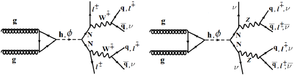
Figure 6: Representative Feynman diagrams for the Higgs portal Majorana neutrino pair production and subsequent decay modes.

Let us now consider the production cross section for the RHNs at the LHC from the $\phi$ and $h$ productions and their decays. Using Eqs. (4.1), (4.2) and (4.10), the cross section formulas are given by

$$\sigma(pp\to\phi\to NN) = \sin^{2}\theta\times\sigma_{h}(m_{\phi})\times BR(\phi\to NN),$$

$$\sigma(pp\to h\to NN) = \cos^{2}\theta\times\sigma_{h}(m_{h})\times BR(h\to NN),$$ (4.11)

respectively, and they are controlled by four parameters, $Y$, $\theta$, $m_{\phi}$ and $m_{N}$. Throughout this section, we fix $m_{N}=20$ GeV, for simplicity. The representative diagrams of the RHN productions including their decays are shown in Fig. 6. We will discuss the decay of RHNs into the SM final states in details in Sec. 5. In the remainder of the analysis in this section, we fix the lifetime of RHNs to yield the best reach of $\sigma_{XX}$ in Fig. 1 for both the future HL-LHC and MATHUSLA displaced vertex searches, namely, $\sigma_{\rm min}({\rm HL-LHC})=20.7$ and $\sigma_{\rm min}({\rm MATH})=0.3$ fb, which corresponds to $c\tau=3.1$ and $58.4$ m, respectively. Here, we identify $X$ with the RHN while $S$ is either $h$ or $\phi$.

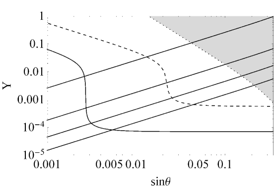
Figure 7: The plots show (i) the best reaches of displaced vertex searches at the HL-LHC (dashed curve) and the the MATHUSLA (dotted curve); (ii) branching ratios of $\phi\to NN$ denoted as the diagonal solid lines ($BR(\phi\to NN)=99.99\%$, $98\%$, $75\%$, and $25\%$, respectively, from top to bottom); (iii) the excluded region (gray shaded) from the LHC constraint on the Higgs branching ratio into the invisible decay mode [67].

We first consider the case where $h$ and $\phi$ masses are almost degenerate, $m_{h}\simeq m_{\phi}=126$ GeV. In this case, the total cross section $\sigma_{XX}$ is given by the sum of the productions from $\phi$ and $h$. The best search reach of the displaced vertex signatures at the HL-LHC or the MATHUSLA are expressed as

$$\sigma_{min} = \sigma(pp\to\phi\to NN)+\sigma(pp\to h\to NN)$$ (4.12)

$$\simeq \left[\sin^{2}\theta\times BR(\phi\to NN)+\cos^{2}\theta\times BR(h\to NN)\right]{\sigma_{h}(m_{h})},$$

where we have used the approximation $\sigma_{h}(m_{\phi})\simeq\sigma_{h}(m_{h})$. Hence, the best search reach is expressed as a function of $Y$ and $\theta$ for the fixed values of $m_{N}=20$ GeV, $m_{h}=125$ GeV and $m_{\phi}=126$ GeV. In Fig. 7, our results are shown in $(Y,\sin\theta)$-plane. This plots show (i) the best reaches of displaced vertex searches at the HL-LHC (dashed curve) and the MATHUSLA (dotted curve); (ii) branching ratios of $\phi\to NN$ denoted as the diagonal solid lines ($BR(\phi\to NN)=99.99\%$, $98\%$, $75\%$, and $25\%$, respectively, from top to bottom); (iii) the excluded region (gray shaded) from the LHC constraint on the Higgs branching ratio into the invisible decay mode, namely,

$${BR}_{\rm inv}^{\rm higgs}=\sin^{2}\theta\times BR(\phi\to NN)+\cos^{2}\theta\times BR(h\to NN)<0.23.$$ (4.13)

Note that along the dashed curve, the RHN pair production is dominated by the decay of $h$ ($\phi$) for $\sin\theta<0.02$ ($\sin\theta>0.02$). Similarly, the RHN pair production is dominated by the decay of $h$ ($\phi$) for $\sin\theta<0.002$ ($\sin\theta>0.002$) along the solid curve.

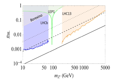
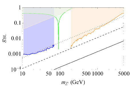
Figure 8: For fixed $Y$ values, the diagonal lines show the the $Z^{\prime}$ boson gauge coupling values as a function of $m_{Z^{\prime}}$, along with the excluded shaded region from various $Z^{\prime}$ boson searches. In the left panel, the three diagonal lines show the results for $Y=0.0181$ (dotted), $3.97\times 10^{-3}$ (dashed) and $4.85\times 10^{-4}$ (solid), respectively, which are chosen from the intersections of the diagonal line for $BR(\phi\to NN)=98\%$ with the solid curve, the dashed curve and dotted line in Fig. 7. The results for the case with $BR(\phi\to NN)=25\%$ are shown in the right panel, where the three diagonal lines correspond to $Y\simeq 3.15\times 10^{-3}$ (dotted), $6.50\times 10^{-4}$ (dashed) and $7.95\times 10^{5}$ (solid), respectively.

In our model, once $Y$ and $m_{N}$ are fixed, the relation between the $B-L$ gauge coupling and the $Z^{\prime}$ boson mass is determined by (see Eq. (3.2))

$$g_{BL}=\frac{1}{2\sqrt{2}}\frac{Y}{m_{N}}m_{Z^{\prime}}.$$ (4.14)

The $Z^{\prime}$ boson has been searched by various experiments, and the upper bound on the $B-L$ gauge coupling as a function of its mass is obtained for a wide mass range of ${\cal O}(1)\lesssim m_{Z^{\prime}}[{\rm GeV}]\leq 5000$. For a $Y$ value chosen in Fig. 7, we examine the consistency with the current constraints from the $Z^{\prime}$ boson search. For several benchmark $Y$ values, we show in Fig. 8 the relation of Eq. (4.14) along with the current experimental constraints from the $Z^{\prime}$ boson searches (the shaded regions are excluded from the result in Ref. [68], the LHCb results [69, 70], and the resent ATLAS results [71]). In the left panel, we show the relation for $Y=0.0181$ (dotted), $3.97\times 10^{-3}$ (dashed) and $4.85\times 10^{-4}$ (solid), which are chosen from the intersections of the diagonal line for $BR(\phi\to NN)=98\%$ with the solid curve, the dashed curve and dotted line in Fig. 7. We find the current constraints from the $Z^{\prime}$ boson search are very severe and complementary to the future search reach of the displaced vertex signatures. In the right panel, we show the relation for $Y\simeq 3.15\times 10^{-3}$ (dotted), $6.50\times 10^{-4}$ (dashed) and $7.95\times 10^{5}$ (solid), which are chosen from the intersections of the diagonal line for $BR(\phi\to NN)=25\%$ with the solid curve, the dashed curve and dotted line in Fig. 7. From the results, we see that if the RHN pair production is dominated by the SM-like Higgs boson decay, the allowed parameter space is very severely constrained except for a window around $m_{Z^{\prime}}=100$ GeV. However, Fig. 8 also shows that we can avoid the constraints by lowering $g_{BL}$.

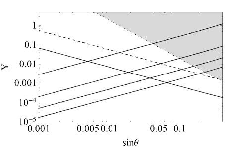
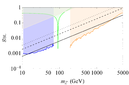
Figure 9: The plots shows the parameter space when the RHNs production at the LHC is dominated by SM Higgs decay for fixed $m_{\phi}=70$ GeV and $m_{N}=20$ GeV. In the left panel, along dashed (solid) diagonal lines with a negative slope, the RHN production cross section at the LHC from the SM Higgs decay is fixed to be the best search reach value for the HL-LHC (MATHUSLA) displaced vertex searches $\sigma(pp\to XX)=20.7(0.3)$ fb in Fig. 1. The gray shaded region are excluded region by the SM Higgs boson invisible decays searches [67]. The plot also shows $BR(\phi\to NN)$ lines, diagonal solid lines with positive slope. From top to bottom, along the line, $BR(\phi\to NN)=99.99\%$, $98\%$, $75\%$, and $25\%$, respectively. In the right panel, for a fixed Y value, the diagonal lines show the the $Z^{\prime}$ boson gauge coupling values as a function of $m_{Z}^{\prime}$, along with the excluded shaded regions from various $Z^{\prime}$ boson searches. The Yukawa values are chosen to satisfy $BR(\phi\to NN)=98\%$ in the left panel. The dotted diagonal line correspond to $Y\simeq 1.90\times 10^{-2}$ is fixed using the intersection of the $BR(\phi\to NN)=98\%$ with the dotted line. Similarly, the dashed (solid) line correspond to $Y\simeq 1.00\times 10^{-2}$ ($3.59\times 10^{-3}$) fixed using the intersection of $BR(\phi\to NN)=98\%$ with the dashed (HL-LHC) and solid (MATHUSLA) lines.

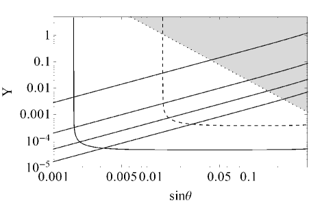
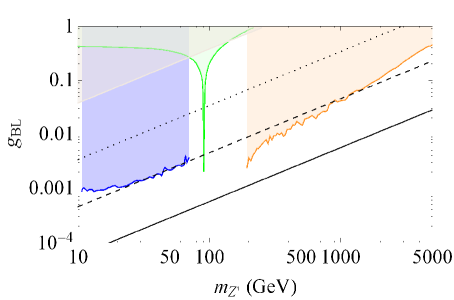
Figure 10: The plots shows the parameter space when the RHNs production at the LHC is dominated by $B-L$ Higgs decay for fixed $m_{\phi}=70$ GeV and $m_{N}=20$ GeV. In the left panel, along dashed (solid) curved lines, the RHN production cross section at the LHC from the SM Higgs decay is fixed to be the best search reach value for the HL-LHC (MATHUSLA) displaced vertex searches $\sigma(pp\to XX)=20.7(0.3)$ fb in Fig. 1. Along the diagonal solid lines with positive slope. $BR(\phi\to NN)$ is fixed. From top to bottom, $BR(\phi\to NN)=99.99\%$, $98\%$, $75\%$, and $25\%$, respectively. The gray shaded region are excluded region by the SM Higgs boson invisible decays searches [67]. In the right panel, for a fixed Y value, the diagonal lines show the the $Z^{\prime}$ boson gauge coupling values as a function of $m_{Z}^{\prime}$, along with the excluded shaded regions from various $Z^{\prime}$ boson searches. The Yukawa values are chosen to satisfy $BR(\phi\to NN)=98\%$ in the left panel. The dotted diagonal line correspond to $Y\simeq 1.92\times 10^{-2}$ is fixed using the intersection of the $BR(\phi\to NN)=98\%$ with the dotted line in the left panel. Similarly, the dashed (solid) line correspond to $Y\simeq 2.58\times 10^{-3}$ and $3.20\times 10^{4}$ fixed using the intersection of $BR(\phi\to NN)=98\%$ with the dashed (HL-LHC) and dashed (MATHUSLA) lines in the left panel

Let us next consider the case that $m_{\phi}$ and $m_{h}$ are well separated. In this case, we calculate the RHN pair productions from the decays of $h$ and $\phi$ separately. For each case, we assume the lifetime of the RHN to yield the best search reach at the HL-LHC or the MATHUSLA shown in Fig. 1. The best search reach of the displaced vertex signatures at the HL-LHC or the MATHUSLA are expressed as $\sigma_{min}=\sigma(pp\to S\to NN)$, where $S$ is either $h$ or $\phi$. Once $m_{\phi}$ is fixed, this equation leads to a relation between $Y$ and $\theta$ as shown in Fig. 7 for $m_{\phi}=126$ GeV. Using Eqs. (2.2), (4.10) and (4.11), we express $\sigma_{min}=\sigma(pp\to S\to NN)$ for $S=\phi$ and $h$, separately, as

$$\Gamma_{NN}(m_{\phi}) = \frac{R(m_{\phi})\tan^{2}\theta}{\sin^{2}\theta-R(m_{\phi})}\left(\Gamma_{SM}(m_{\phi})+\frac{\Gamma(\phi\to hh)}{\sin^{2}\theta}\right),$$

$$\Gamma_{NN}(m_{h}) = \frac{R(m_{h})\cot^{2}\theta}{\cos^{2}\theta-R(m_{h})}\Gamma_{SM}(m_{h}),$$ (4.15)

where $R$ is defined as

$$R(m_{S})=\frac{\sigma_{min}}{\sigma_{h}(m_{S})}.$$ (4.16)

Using Eqs. (4.6) and $(\ref{eq: dw})$, we then obtain the relation between $Y$ and $\theta$ for each case as follows:

$$Y^{2} = \frac{16\pi}{3}\frac{\tan^{2}\theta}{\sin^{2}\theta-R(m_{\phi})}\left(\frac{R(m_{\phi})}{m_{\phi}}\right)\left(\Gamma_{{SM}}(m_{\phi})+\frac{\Gamma(\phi\to hh)}{\sin^{2}\theta}\right)\left(1-\frac{4m_{N}^{2}}{m_{\phi}^{2}}\right)^{-3/2},$$

$$Y^{2} = \frac{16\pi}{3}\frac{\cot^{2}\theta}{\cos^{2}\theta-R(m_{h})}\left(\frac{R(m_{h})}{m_{h}}\right)\;\Gamma_{{SM}}(m_{h})\left(1-\frac{4m_{N}^{2}}{m_{h}^{2}}\right)^{-3/2}.$$ (4.17)

The first equation in Eq. (4.17) indicates that for a fixed $R(m_{\phi})<1$, $Y^{2}$ becomes singular for $\sin^{2}\theta=R(m_{\phi})$. Thus, there is a lower bound on $\sin\theta$ to achieve the best reach cross section $\sigma_{\rm min}$. For $\sin\theta\sim 1$, $Y^{2}$ becomes singular in both the equations. However, such a large mixing angle is excluded by the measurement of the SM Higgs boson properties at the LHC.

In Fig. 9, we show our results for the case that the RHNs are produced from the SM-like Higgs boson decay. Here, we have fixed $m_{\phi}=70$ GeV and $m_{N}=20$ GeV. In the left panel, the best reach cross section at the HL-LHC (MATHUSLA) is achieved along the dashed (solid) diagonal line with a negative slope. The four solid diagonal lines with positive slopes denote the relations between $Y$ and $\sin\theta$ to yield $BR(\phi\to NN)=99.99\%$, $98\%$, $75\%$, and $25\%$, respectively, from top to bottom. The gray shaded region is excluded by the LHC constraint on the Higgs branching ratio into the invisible decay mode [67], which is simply given by

$${BR}_{\rm inv}^{\rm higgs}=\cos^{2}\theta\times BR(h\to NN)<0.23,$$ (4.18)

for the present case. The right panel corresponds to Fig. 8. The three diagonal lines corresponds $Y\simeq 1.90\times 10^{-2}$ (dotted), $Y\simeq 1.00\times 10^{-2}$ (dashed) and $3.59\times 10^{-3}$ (solid), respectively, which are chosen from the intersections of the diagonal line for $BR(\phi\to NN)=98\%$ with the solid, dashed and dotted lines with negative slopes in the left panel.

Fig. 10 shows the results corresponding to Fig. 8, but for the case that the RHNs are produced from the $B-L$ Higgs boson decay, with $m_{\phi}=70$ GeV and $m_{N}=20$ GeV. Along the dashed and solid curves, the best reach cross section is achieved at the HL-LHC and the MATHUSLA, respectively. The four solid diagonal lines with positive slopes denote the relations between $Y$ and $\sin\theta$ to yield $BR(\phi\to NN)=99.99\%$, $98\%$, $75\%$, and $25\%$, respectively, from top to bottom. The gray shaded region is excluded region by the SM Higgs boson invisible decays search. As we have discussed, the curves show the singularities for small $\sin\theta$ values. In the right panel, the three diagonal lines corresponds $Y\simeq 1.92\times 10^{-2}$ (dotted), $Y\simeq 2.58\times 10^{-3}$ (dashed) and $3.20\times 10^{-4}$ (solid), respectively, which are chosen from the intersections of the diagonal line for $BR(\phi\to NN)=98\%$ with the solid curve, the dashed curve and the dotted line in the left panel.

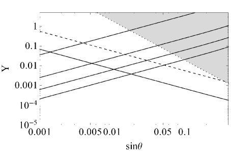
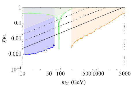
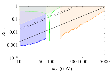
Figure 11: For fixed $m_{\phi}=200$ GeV and $m_{N}=20$ GeV, the plots shows the parameter space when the RHNs production at the LHC is from the: SM Higgs decay (top panel) and $B-L$ decay (bottom panel). The line coding for plots in the top and bottom panels is the same as Figures 9 and 10, respectively. For the plots in the top (bottom) right column, the branching ratio in fixed to be, $BR(\phi\to NN)=98\%$ with a corresponding $Y\simeq 1.03\times 10^{-1},3.68\times 10^{-2}$ and $1.28079\times 10^{-2}$ ($Y\simeq 1.03\times 10^{-1},8.12\times 10^{2}$ and $1.01\times 10^{-2}$), for dotted, dashed, and solid lines, respectively.

Our results for $m_{\phi}=200$ GeV corresponding to Figs. 9 and 10 are shown, respectively, in the top panels and the bottom panels of Fig. 11. All line and color codings are the same as Figs. 9 and 10. In the top-right (bottom-right) panel, three diagonal lines correspond to $Y\simeq 1.03\times 10^{-1}$, $Y=3.68\times 10^{-2}$ and $Y=1.28\times 10^{-2}$ ($Y\simeq 1.03\times 10^{-1}$, $Y=8.12\times 10^{-1}$ and $1.01\times 10^{-2}$), respectively, from top to bottom. Fig. 12 is the same as Fig. 11 but for $m_{\phi}=400$ GeV. Note that in this case, the total decay width also includes the decay mode of $\phi\to hh$. In the top-right (bottom-right) panel, three diagonal lines correspond to $Y\simeq 2.38\times 10^{-1}$, $Y=6.86\times 10^{-2}$ and $Y=2.32\times 10^{-2}$ ($Y\simeq 2.38\times 10^{-1}$, $Y=3.94\times 10^{-1}$ and $4.79\times 10^{-2}$), respectively, from top to bottom. Qualitative behaviors of various curves and lines shown in this figure are similar to those in Fig. 11.

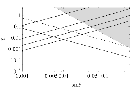
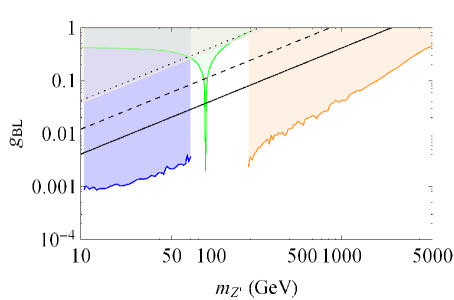
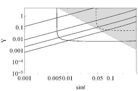
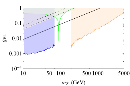
Figure 12: For fixed $m_{\phi}=400$ GeV and $m_{N}=20$ GeV, the plots shows the parameter space when the RHNs production at the LHC is from the: SM Higgs decay (top panel) and $B-L$ decay (bottom panel). The line coding for the top and bottom panels is the same as Figures 9 and 10, respectively. For the plots in the top (bottom) right column, the branching ratio in fixed to be, $BR(\phi\to NN)=98\%$ with a corresponding $Y\simeq 2.38\times 10^{-1},6.86\times 10^{-2}$ and $2.32\times 10^{-2}$ ($Y\simeq 2.38\times 10^{-1},3.94\times 10^{-1}$ and $4.79\times 10^{-2}$), for dotted, dashed, and solid lines, respectively.

Let us here summarize our results as $m_{\phi}$ is increased. From the left panel in Fig. 10, the bottom-left panels in Fig. 11 and Fig. 12, we can see that the resultant curves and the diagonal lines are shifting upward to the right as $m_{\phi}$ is increased. This is because (i) as $m_{\phi}$ is increased, the partial decay widths of $\phi$ into the SM particles become larger and as a result, $Y$ is increased to yield a fixed branching ratio to $\phi\to NN$, see Eq. 4.17; (ii) since $\sigma_{h}(m_{\phi})$ is decreasing as $m_{\phi}$ is increased, the lower bound on $\sin\theta$ (at which $Y$ becomes singular) is increasing (see the discussion below Eq. (4.17). Hence, the LHC constraint from the invisible decay of the SM Higgs boson relatively becomes more severe. In fact, the bottom-left panel of Fig. 12 shows that the dashed curve appears inside the gray shaded region and thus the entire parameter region which can be explored at the future HL-LHC is already excluded. According to Eq. 4.14, the $B-L$ gauge coupling becomes larger for a fixed $m_{Z^{\prime}}$ as $Y$ becomes larger. Hence, the current constraints from the $Z^{\prime}$ boson search become more severe as $m_{\phi}$ is increased as can be seen from the right panel in Fig. 10, the bottom-right panel in Fig. 11 and the bottom-right panel in Fig. 12. Note that if we take $g_{BL}$ small enough, for example, $g_{BL}<10^{-4}$, all the existing collider constraints from the $Z^{\prime}$ boson search can be avoided.

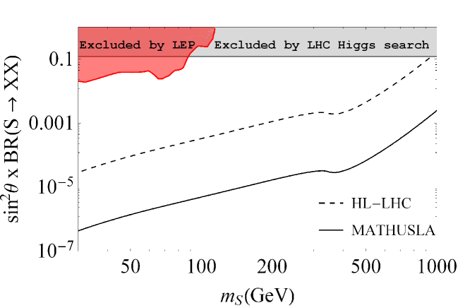
Figure 13: The search reach of the displaced vertex searches at the HL-LHC and MATHUSLA. For $BR(S\to XX)\simeq 100\%$, the red (gray) shaded region is excluded by the LEP (LHC) experiments.

We conclude this section by generalizing our analysis for the long-lived heavy neutrino to the case for an SM-singlet particle $X$ produced through $pp\to S\to XX$ with an SM-singlet scalar $S$ at the LHC. Since $S$ is SM-singlet, it is produced at the LHC through a mixing with the SM Higgs boson, just like $\phi$. Hence, the total production cross section of the process, $pp\to S\to XX$, is given by

$$\sigma(pp\to S\to XX) = \sigma(pp\to S)\times BR(S\to XX)$$ (4.19)

$$= \sin^{2}\theta\times\sigma_{h}(m_{S})\times BR(S\to XX),$$

where $\theta$ is the mixing angle, and $\sigma_{h}(m_{S})$ is the production cross section of the SM Higgs boson if the SM Higgs boson mass were the mass of $S$ ($m_{S}$). Let us assume the lifetime of $X$ to yield the best reach values, $\sigma_{\rm min}({\rm HL-LHC})=20.7$ and $\sigma_{\rm min}({\rm MATHUSLA})=0.310$ fb, for the displaced vertex searches at the HL-LHC and the MATHUSLA, respectively. We then calculate $\sigma_{h}(m_{S})$ at the 13 TeV LHC to obtain a relation between $\sin^{2}\theta\times BR(S\to XX)$ and $m_{S}$ to achieve the best reach value $\sigma(pp\to S\to XX)=\sigma_{\rm min}({\rm HL-LHC})$ or $\sigma_{\rm min}({\rm MATHUSLA})$. Our results are shown in Fig. 13. The region above the dashed black line (solid black line) can be explored at the HL-LHC (the MATHUSLA) with a $3\rm~{}ab^{-1}$ luminosity. For the case of $BR(S\to XX)\simeq 100\%$, the red shaded region is excluded by the LEP results on the search for the SM Higgs boson, while the gray shaded region is excluded by the LHC measurement of the SM Higgs boson properties. Assuming $BR(S\to XX)\simeq 100\%$, we can read off the search reach of $m_{S}$ from Fig. 13 for a fixed value of $\sin\theta$. Our results for three benchmark points are listed in Table 2.

Benchmark Points	Mixing angle ($\theta$)	Search Reach of $m_{S}$[GeV]
		MATHUSLA	HL-LHC
BP1	8 $\times 10^{-3}$	476	39
BP2	5 $\times 10^{-2}$	972	293
BP3	$1\times 10^{-2}$	556	65

Table 2: Summary of $\phi$ mass reach at MATHUSLA and HL-LHC experiment.

5 Lifetime of heavy neutrinos

We assumed a suitable lifetime of the heavy neutrino in the previous section. In this section, we calculate the lifetime of the heavy neutrinos for realistic parameters to reproduce the neutrino oscillation data and investigate the prospect of searching for the displaced vertex signatures of the heavy neutrino productions.

After the $B-L$ and electroweak symmetry breakings, the neutrino mass matrix is generated to be

$${\cal M}_{\nu}=\begin{pmatrix}0&&m_{D}\\ (m_{D})^{T}&&M_{N}\end{pmatrix},$$ (5.1)

where $M_{N}$ and $m_{D}$ are the Majorana and the Dirac mass matrices, respectively. From Eqs. (3.1) and (3.2), we have $M_{N}={\rm diag}(m_{N^{1}},m_{N^{2}},m_{N^{3}})$ and $m_{D}^{ij}=Y_{D}^{ij}v_{SM}/\sqrt{2}$. Assuming the mass hierarchy $|m_{D}^{ij}/m_{N^{k}}|\ll 1$, the seesaw formula for the light Majorana neutrinos is given by

$$m_{\nu}\simeq-m_{D}(M_{N})^{-1}m_{D}^{T}.$$ (5.2)

The light neutrino flavor eigenstate $(\nu)$ can be expressed in terms the light $(\nu_{m})$ and heavy $(N_{m})$ Majorana neutrino mass eigenstates, $\nu\simeq\mathcal{N}\nu_{m}+\mathcal{R}N_{m}$, where $\mathcal{R}=m_{D}(M_{N})^{-1}$, $\mathcal{N}=\Big{(}1-\frac{1}{2}\mathcal{R}^{\ast}\mathcal{R}^{T}\Big{)}\simeq U_{\rm{MNS}}$, and $U_{\rm{MNS}}$ is the neutrino mixing matrix which diagonalizes $m_{\nu}$ by

$$U_{\rm MNS}^{T}m_{\nu}U_{\rm MNS}=D_{\nu}={\rm diag}(m_{1},m_{2},m_{3}),$$ (5.3)

where the neutrino mixing matrix is parameterized as

$$U_{\rm{MNS}}=\begin{pmatrix}c_{12}c_{13}&c_{12}c_{13}&s_{13}e^{-i\delta}\\ -s_{12}c_{23}-c_{12}s_{23}s_{13}e^{i\delta}&c_{12}c_{23}-s_{12}s_{23}s_{13}e^{i\delta}&s_{23}c_{13}\\ s_{12}c_{23}-c_{12}c_{23}s_{13}e^{i\delta}&-c_{12}s_{23}-s_{12}c_{23}s_{13}e^{i\delta}&c_{23}c_{13}\end{pmatrix}\begin{pmatrix}1&0&0\\ 0&e^{-i\rho_{1}}&0\\ 0&0&e^{-i\rho_{2}}\end{pmatrix},$$ (5.4)

where $c_{ij}=\cos\theta_{ij}$, $s_{ij}=\sin\theta_{ij}$, $\delta$ is the Dirac $CP$ phase, and $\rho_{1}$ and $\rho_{2}$ are the Majorana $CP$ phases. Using the Eqs. (5.2) and (5.3), the Dirac mass matrix is parameterized as [72]

$$m_{D}=U_{\rm{MNS}}^{*}\sqrt{D_{\nu}}\;O\sqrt{M_{N}},$$ (5.5)

where $O$ is a general orthogonal matrix, $\sqrt{M_{N}}\equiv{\rm diag}(\sqrt{m_{N^{1}}},\sqrt{m_{N^{2}}},\sqrt{m_{N^{3}}})$ and $\sqrt{D_{\nu}}\equiv{\rm diag}(\sqrt{m_{1}},\sqrt{m_{2}},\sqrt{m_{3}})$.

The charged current interaction of the neutrino mass eigenstates is expressed as

$$\mathcal{L}_{CC}=-\frac{g}{\sqrt{2}}W_{\mu}\overline{\ell_{\alpha}}\gamma^{\mu}P_{L}\left({\cal N}_{\alpha i}\nu_{m}^{i}+{\cal R}_{\alpha i}N_{m}^{i}\right)+\rm{h.c.},$$ (5.6)

where $\ell_{\alpha}$ are the 3 generations of the charged SM leptons, and $P_{L}=(1-\gamma_{5})/2$ is the left handed projection operator. Similarly, for the the neutral current interaction, we have

$$\mathcal{L}_{NC} = -\frac{g}{2\cos\theta_{\rm W}}Z_{\mu}\Big{[}\overline{\nu_{m}^{i}}\gamma^{\mu}P_{L}({\cal N}^{\dagger}{\cal N})_{ij}\nu_{m}^{j}+\overline{N_{m}^{i}}\gamma^{\mu}P_{L}({\cal R}^{\dagger}{\cal R})_{ij}N_{m}^{j}$$ (5.7)

$$+ \Big{\{}\overline{\nu_{m}^{i}}\gamma^{\mu}P_{L}({\cal N}^{\dagger}{\cal R})_{ij}N_{m}^{j}+\rm{H.c.}\Big{\}}\Big{]},$$

where $\theta_{\rm W}$ is the weak mixing angle.

With the general parameterization of Eq. (5.5), the matrix ${\mathcal{R}}$ is given by

$$R_{\alpha i}=m_{D}(M_{N})^{-1}=U_{\rm{MNS}}^{*}\sqrt{D_{\nu}}\;O(\sqrt{M_{N}})^{-1}.$$ (5.8)

In order to fix $R_{\alpha i}$, we employ the neutrino oscillation data: $\sin^{2}2{\theta_{13}}=0.092$ [73] along with $\sin^{2}2\theta_{12}=0.87$, $\sin^{2}2\theta_{23}=1.0$, as well as the mass squared differences, $\Delta m_{12}^{2}=m_{2}^{2}-m_{1}^{2}=7.6\times 10^{-5}$ eV² and $\Delta m_{23}^{2}=|m_{3}^{2}-m_{2}^{2}|=2.4\times 10^{-3}$ eV² [3]. Motivated by the recent measurements, we also fix the Dirac $CP$ phase as $\delta=\frac{3\pi}{2}$ [74], while we simply take $\rho_{1}=\rho_{2}=0$ for the Majorana $CP$ phases. To simplify our analysis, we set the orthogonal matrix $O$ to be the identity matrix and assume the mass degeneracy for three heavy neutrinos, $m_{N^{1,2,3}}=m_{N}$. For the light neutrino mass spectrum, we consider two cases: the normal hierarchy (NH), $m_{1}<m_{2}<m_{3}$, and the inverted hierarchy (IH), $m_{3}<m_{1}<m_{2}$.

Let us now consider the decay of the heavy neutrinos into the SM particles. In our analysis, we set $m_{N}=20$ GeV, hence the heavy neutrino decays into the SM quarks and leptons via intermediate off-shell $W$ and $Z$ bosons. The expression for the decay width of heavy neutrinos into various final states are as follows:

1. Leptons in the final states:

$$\Gamma^{(W)}({N^{i}\to\ell_{L}^{\alpha}\ell_{L}^{\beta}\nu^{\kappa}}) = \left(\sum_{\alpha=1}^{3}|R_{\alpha i}|^{2}\right)\left(\sum_{\beta,\kappa}|U^{\beta\kappa}_{MNS}|^{2}\right)\Gamma_{\rm N^{i}},$$

$$\Gamma^{(Z)}({N^{i}\to\nu^{\alpha}\ell_{L}^{\beta}\ell_{L}^{\kappa}}) = \left(\sum_{\alpha=1}^{3}|R_{\alpha i}|^{2}\right)\left(\sum_{\beta,\kappa=1}\delta_{\beta\kappa}\right)\cos^{2}2\theta_{W}\,\frac{1}{4}\,\Gamma_{\rm N^{i}},$$

$$\Gamma^{(Z)}({N^{i}\to\nu^{\alpha}\ell_{R}^{\beta}\ell_{R}^{\kappa}}) = \left(\sum_{\alpha=1}^{3}|R_{\alpha i}|^{2}\right)\left(\sum_{\beta,\kappa}\delta_{\beta\kappa}\right)\,\sin^{4}\theta_{W}\,\Gamma_{\rm N^{i}},$$

$$\Gamma^{(Z)}({N^{i}\to\nu^{\alpha}\nu^{\beta}\nu^{\kappa}}) = \left(\sum_{\alpha=1}^{3}|R_{\alpha i}|^{2}\right)\left(\sum_{\beta,\kappa}\delta_{\beta\kappa}\right)\,\frac{1}{4}\,\Gamma_{\rm N^{i}},$$ (5.9)

where

$$\Gamma_{\rm N^{i}}=\frac{G_{F}^{2}}{192\pi^{3}}m_{N^{i}}^{5}$$ (5.10)

with the Fermi constant $G_{F}$, $U_{MNS}^{\alpha\beta}$ is a $(\alpha,\beta)$-element of the neutrino mixing matrix, and $\sum_{\beta,\kappa}|U^{\beta\kappa}_{MNS}|^{2}=3=\sum_{\beta,\kappa}\delta_{\beta\kappa}$. In deriving the above formulas, we have neglected all lepton masses. For a degenerate heavy neutrino mass spectrum, we obtain $\sum_{\alpha=1}^{3}|R_{\alpha i}|^{2}=\frac{m_{i}}{m_{N}}$. For the lepton final states, we have an interference between the $Z$ and $W$ boson mediated decay processes:

$$\Gamma^{(Z/W)}({N^{i}\to\nu\ell\ell}) = \left(\sum_{\alpha=1}^{3}|R_{\alpha i}|^{2}\right)\times 2{\rm Re}(U_{ii})\times\Gamma_{\rm N^{i}}.$$ (5.11)

2. Quarks in the final states:

$$\Gamma^{(W)}(N^{i}\to\ell^{\alpha}q_{L}^{\beta}{\bar{q}}_{L}^{\kappa}) = N_{c}\left(\sum_{\alpha=1}^{3}|R_{\alpha i}|^{2}\right)\left(\sum_{\beta,\kappa}|V^{q^{\beta}{\bar{q}}^{\kappa}}_{CKM}|^{2}\right)\Gamma_{\rm N^{i}},$$

$$\Gamma^{(Z)}(N^{i}\to\nu^{\alpha}q_{L}^{\beta}{\bar{q}}_{L}^{\kappa}) = N_{c}\left(\sum_{\alpha=1}^{3}|R_{\alpha i}|^{2}\right)\left(\sum_{\beta,\kappa}|V^{q^{\beta}{\bar{q}}^{\kappa}}_{CKM}|^{2}\right)\cos^{2}2\theta_{W}\,\frac{1}{4}\,\Gamma_{\rm N^{i}},$$

$$\Gamma^{(Z)}(N^{i}\to\nu^{\alpha}q_{R}^{\beta}{\bar{q}}_{R}^{\kappa}) = N_{c}\left(\sum_{\alpha=1}^{3}|R_{\alpha i}|^{2}\right)\left(\sum_{\beta,\kappa}|V^{q^{\beta}{\bar{q}}^{\kappa}}_{CKM}|^{2}\right)\,\sin^{4}\theta_{W}\,\Gamma_{\rm N^{i}},$$ (5.12)

where $N_{c}=3$ is the color factor. Since we have set $m_{N}=20$ and $40$ GeV in the following analysis, we only consider the first two generation of quarks in the final states and $\sum_{\beta,\kappa}|V^{q^{\beta}{\bar{q}}^{\kappa}}_{CKM}|^{2}=2$. For the final state quarks, there is no interference between $W$ and $Z$ boson mediated processes.

Figure 14: The left (right) panel shows the decay lengths of heavy neutrinos as a function of the lightest light neutrino mass $m_{1}$ ($m_{3}$), for the NH (IH) case. In both panels, the dotted, dashed, and the solid lines correspond to the decay lengths of $N^{1},N^{2}$, and $N^{3}$, respectively, with $m_{N}=20$ GeV. In the right panel, the dotted and dashed lines are indistinguishable.

Using Eqs. (5.9), (5.11), and (5.12), we evaluate the total decay width of each heavy neutrino ($\Gamma_{N^{i}}$). The decay length (in meters) are found to be

$$c\tau_{1} = \frac{1}{\Gamma_{N^{1}}}\simeq 6.98\times 10^{5}\frac{1}{\;m_{N}^{4}\;m_{1}},$$

$$c\tau_{2} = \frac{1}{\Gamma_{N^{2}}}\simeq 7.25\times 10^{5}\frac{1}{\;m_{N}^{4}\;m_{2}},$$

$$c\tau_{3} = \frac{1}{\Gamma_{N^{3}}}\simeq 7.11\times 10^{5}\frac{1}{\;m_{N}^{4}\;m_{3}},$$ (5.13)

where $m_{N}$ is in units of GeV while $m_{i}$ is in units of eV. The decay length $c\tau_{i}$ is inversely proportional to $m_{i}$ because of $\Gamma_{N^{i}}\propto\sum_{\alpha=1}^{3}|R_{\alpha i}|^{2}=\frac{m_{i}}{m_{N}}$. For the NH and IH cases, the decay lengths for the heavy neutrinos $N^{1,2,3}$ are plotted in Fig. 14 as a function of the lightest light neutrino mass.

Figure 15: For the NH case, the search reach cross sections with $m_{\phi}=126$ GeV and $m_{N}=20$ GeV along with the heavy neutrino decay lengths for the three benchmark $m_{\rm lightest}$ values (vertical lines). The top-left, top-right and bottom panels are for $m_{\rm lightest}=m_{1}=0.1$, $0.01$ and $0.001$ eV, respectively

Figure 16: Same as Fig. 15 but for the IH case. The top-left, top-right and bottom panels are for $m_{\rm lightest}=m_{3}=0.1$, $0.01$ and $0.001$ eV, respectively

In Fig. 14, let us consider three benchmark values for the lightest light neutrino mass as $m_{\rm lightest}=0.1$, $0.01,$ and $0.001$ eV. For each benchmark $m_{\rm lightest}$ value, the decay lengths for the three heavy neutrinos are fixed. It is then interesting to combine the benchmark decay lengths with the search reach of the displaced vertex signatures at the future colliders. For the NH case, we show in Fig. 15 the search reach cross sections with $m_{\phi}=126$ GeV and $m_{N}=20$ GeV along with the heavy neutrino decay lengths for the three benchmark $m_{\rm lightest}$ values (vertical lines). The top-left, top-right and bottom panels are for $m_{\rm lightest}=m_{1}=0.1$, $0.01$ and $0.001$ eV, respectively Interestingly, for all benchmarks, the value of $c\tau_{3}$ is very close to the lifetime yielding the best reach cross section at the MATHUSLA. Same as Fig. 15 but for the IH case is shown in Fig. 16. The top-left, top-right and bottom panels are for $m_{\rm lightest}=m_{3}=0.1$, $0.01$ and $0.001$ eV, respectively For all benchmarks, the value of $c\tau_{1}$ is very close to the lifetime yielding the best reach cross section at the MATHUSLA.

The heavy neutrino lifetimes become shorter as $m_{\rm lightest}$ is raised (see Eq. (5.13)). However, if we consider the cosmological bound on the sum of the light neutrino masses, $\sum m_{\rm lightest}=0.23$ MeV [75], we obtain the lower bound on the decay length to be $c\tau\gtrsim 20$ m. In fact, this lower bound can be significantly reduced if we consider the complex orthogonal matrix $O$ in the general parametrization. See, for example, Ref. [76].

In the previous section, we have shown the relation between $Y$ and $\sin\theta$ to achieve the best reach cross section at the HL-LHC/MATHUSLA, assuming the heavy neutrino lifetime to be the best point for each experiment. To conclude this section, we repeat the same analysis in the previous section but for various values of $c\tau$ determined by $m_{\rm lightest}$ values. For this analysis, we set $m_{N}=40$ GeV and $m_{\phi}=150$ GeV. The decay lengths of heavy neutrinos for this parameter choice are depicted in Fig. 17. In this case, the cosmological lower bound on $c\tau$ is found to be $c\tau\simeq 1.3$ m.

Figure 17: Same as Fig. 14 but for the case with $m_{N}=40$ GeV.

In Fig. 18, we show our results corresponding to the top-left and bottom-left panels in Fig. 11. The left panel corresponds to the the top-left panel of Fig. 11. Here, we consider the heavy neutrino production from the SM-like Higgs decay and the search reach at the HL-LHC. The diagonal dashed lines from left to right are results correspond to $m_{\rm lightest}=8.90\times 10^{-2}$, $10^{-2}$, $5.00\times 10^{-3}$ and $10^{-3}$ eV, or equivalently $c\tau=3.10$, $27.2$, $54.0$ and $273$ m. The solid diagonal lines denote the relations between $Y$ and $\sin\theta$ to yield $BR(\phi\to NN)=99.99\%$, $98\%$, $75\%$, and $25\%$, respectively, from top to bottom. The gray shaded region is excluded by the LHC constraint on the invisible Higgs decay. The right panel corresponds to the the bottom-left panel of Fig. 11. Here, we consider the heavy neutrino production from the $B-L$ Higgs decay. The line coding are the same as the left panel. The parameter region for $m_{\rm lightest}\lesssim 10^{-3}$ eV is already excluded.

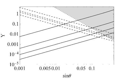
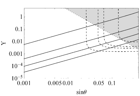
Figure 18: For fixed $m_{\phi}=150$ GeV and $m_{N}=40$ GeV and for different $m_{\rm lightest}$ values, the plots show the parameter space for displaced vertex search at HL-LHC when the RHNs are produced from: SM Higgs decay (left) and $B-L$ decay (right). For both the panels, from left to right, the dashed lines correspond to $m_{\rm lightest}\simeq 8.90\times 10^{-2},10^{-2},5.00\times 10^{-3}$, and $10^{-3}$ eV, or equivalently $c\tau=273,54.0,27.2$, and $3.10$ m, respectively. In both panels, from top to bottom, the solid lines are correspond to fixed $BR(\phi\to NN)=99.99\%$, $98\%$, $75\%$, and $25\%$, respectively. Similarly, the gray shaded region are excluded region by the SM Higgs boson invisible decay searches.

Same as Fig. 18 but for the search reach at the MATHUSLA is shown in Fig. 19. Solid diagonal lines with negative slope in the left panel and the solid curves in the right panel correspond to $m_{\rm lightest}\simeq 10^{-1}$, $4.61\times 10^{-3}$, $5.00\times 10^{-4}$ and $10^{-4}$ eV, or equivalently $c\tau=2.73$, $59.1$, $545$ and $2.73\times 10^{3}$ m, from left to right. The line coding for the other lines and the shaded region are the same as Fig. 18.

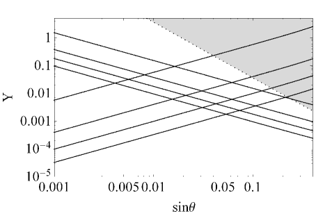
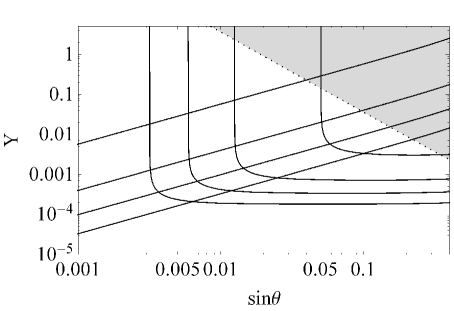
Figure 19: For fixed $m_{\phi}=150$ GeV and $m_{N}=40$ GeV and for different $m_{\rm lightest}$ values, the plots show the parameter space for displaced vertex search at MATHUSLA when the RHNs are produced from: SM Higgs decay (left) and $B-L$ decay (right). For both the panels, from left to right, the dashed lines correspond to $m_{\rm lightest}\simeq 10^{-1},4.61\times 10^{-3},5.00\times 10^{-4}$, and $10^{-4}$ eV, or equivalently $c\tau=2.73\times 10^{3},59.1,545$, and $2.73$ m, respectively. The line coding for the remaining curves and regions are same as Fig. 18.

6 Complementarity to neutrinoless double beta decay search

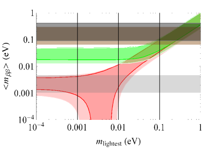
Figure 20: In the left panel, the red and the green shaded region correspond to the constraint on effective netrino mass ($\langle m_{\beta\beta}\rangle$) for the NH and IH, respectively. The horizontal shaded regions from the top to bottom, correspond to the current EXO-200 experiment and the future reach of EXO-200 phase-II, and nEXO experiments, respectively [77]. In the right panel, the solid line depicts the total decay length of RHN plotted against the mass of the corresponding lightest light-neutrino mass. The dashed (solid) line correspond to fixed RHN mass of $20$ ($40$) GeV. In both the panels, vertical solid lines correspond to the three benchmark points for the lightest neutrino masses for the NH and the IH, namely, $m_{\rm lightest}=0.1,0.01,$ and $0.001$ eV.

The neutrinoless double beta decay of heavy nuclei is a “smoking-gun" signature of the Majorana nature of neutrinos. In this process, two neutrons in nuclei simultaneously decay into two protons plus two electrons without emitting neutrinos, and hence the lepton number is violated by two units. The neutrinoless double beta decay process is characterized by an effective mass of the light neutrino ($\langle m_{\beta\beta}\rangle$) defined as

$$\langle m_{\beta\beta}\rangle=\left|\sum_{j}m_{j}U_{ej}^{2}\right|,$$ (6.1)

where $U_{ej}$ is the $(e,j)$-element of the neutrino mixing matrix $U_{\rm MNS}$, see [77] for review of neutrinoless double beta decay. Employing the current neutrino oscillation data, the effective mass is described by the lightest light neutrino mass. The left panel in Fig. 20 depicts the relation between $\langle m_{\beta\beta}\rangle$ and $m_{\rm lightest}$ for the NH (red shaded region) and IH (green shaded region) cases. In this panel, the current upper limit by the EXO-200 experiment (upper horizontal shaded region) and the future reach by the EXO-200 phase-II and nEXO experiments (lower horizontal shaded region) are also shown.

As we have investigated in the previous section, the decay lengths of the heavy neutrinos are controlled by $m_{\rm lightest}$. In the right panel of Fig. 20, we show the decay length of the heavy neutrino $N^{3}$ for the NH case as a function of $m_{\rm lightest}$. The dashed and solid lines correspond to the heavy neutrino masses of $m_{N}=20$ and $40$ GeV, respectively. In Fig. 20, our benchmarks of $m_{\rm lightest}=0.1$, $0.01$ and $0.001$ are depicted by the vertical lines. It is interesting to compare the two panels. If the displaced vertex from a heavy neutrino decay is observed and the heavy neutrino mass is reconstructed from its decay products, $m_{\rm lightest}$ is determined. If the neutrinoless double beta decay is observed, $\langle m_{\beta\beta}\rangle$ is measured. However, if $\langle m_{\beta\beta}\rangle$ is measured to be around $0.03$ eV or $0.002$ eV, $m_{\rm lightest}$ is left undetermined. Hence, the observations of the displaced vertex and the neutrinoless double beta decay are complementary with each other.

7 Conclusions

It is quite possible that new particles in new physics beyond the SM are completely singlet under the SM gauge group. This is, at least, consistent with the null results on the search for new physics at the LHC. If this is the case, we may expect that such particles very weakly couple with the SM particles and thus have a long lifetime. Such particles, once produced at the high energy colliders, provide us with the displaced vertex signature, which is very clean with negligible SM background. In the context of the minimal gauged $B-L$ extended SM, we have considered the prospect of searching for the heavy neutrinos of the type-I seesaw mechanism at the future high energy colliders. For the production process of the heavy neutrinos, we have investigated the production of Higgs bosons and their subsequent decays into a pari of heavy neutrinos. With the parameters reproducing the neutrino oscillation data, we have shown that the heavy neutrinos are long-lived and their displaced vertex signatures can be observed at the next generation displaced vertex search experiments, such as the HL-LHC, the MATHUSLA, the LHeC, and the FCC-eh. We have found that the lifetime of the heavy neutrinos is controlled by the lightest light neutrino mass, which leads to a correlation between the displaced vertex search and the search limit of the future neutrinoless double beta-decay experiments.

Note added: While completing this manuscript, we noticed a paper by F. Deppisch, W. Liu and M. Mitra [78] which also considers the displaced vertex signature of the heavy neutrinos.

8 Appendix

The partial decay widths of various decay modes of the SM-like Higgs boson of mass $m_{h}$ is given by [79] :

(i) SM fermions (f):

$$\Gamma_{h\to f{\bar{f}}} = \cos^{2}{\theta}\times\frac{3N_{f}m_{h}m_{f}^{2}}{8\pi v_{SM}^{2}}\left(1-\frac{4m_{f}^{2}}{m_{h}^{2}}\right)^{3/2},$$

where $f$ are the SM fermions and $N_{f}=1$ and $3$ for SM leptons and quarks, respectively.

(ii) on-shell gauge bosons (V = W or Z):

$$\Gamma_{h\to VV} = \cos^{2}{\theta}\times\frac{C_{V}}{32\pi}\frac{m_{h}^{3}}{v_{SM}^{2}}\left(1-4\frac{m_{V}^{2}}{m_{h}^{2}}\right)^{1/2}\left(1-4\frac{m_{V}^{2}}{m_{h}^{2}}+12\left(\frac{m_{V}^{2}}{m_{h}^{2}}\right)^{2}\right),$$

where $C_{V}=1$ and $2$ for $V=Z$ or $W$ gauge boson, respectively.

(iii) gluon (g) via top-quark loop:

$$\Gamma_{h\to gg} = \cos^{2}{\theta}\times\frac{\alpha_{s}^{2}m_{h}^{3}}{128\pi^{3}v^{2}}(F_{1/2}(m_{h}))^{2},$$

where

$$F_{1/2}(m_{h}) = -2\frac{4m_{t}^{2}}{m_{h}^{2}}\left[1-\left(1-\frac{4m_{t}^{2}}{m_{h}^{2}}{\rm arcsin}^{2}\left(\frac{m_{h}}{2m_{t}}\right)\right)\right].$$

(iii) one off-shell gauge boson :

$$\Gamma_{h\to WW^{*}} = \cos^{2}{\theta}\times\frac{3m_{W}^{4}m_{h}}{32\pi^{3}v_{SM}^{4}}G\left(\frac{m_{W}^{2}}{m_{h}^{2}}\right),$$

$$\Gamma_{h\to ZZ^{*}} = \cos^{2}{\theta}\times\frac{3m_{Z}^{4}m_{h}}{32\pi^{3}v_{SM}^{4}}\left(\frac{7}{12}-\frac{10}{9}\sin^{2}\theta_{W}+\frac{40}{9}\sin^{4}\theta_{W}\right)G\left(\frac{m_{W}^{2}}{m_{h}^{2}}\right),$$ (8.1)

where $\sin^{2}\theta_{W}=0.231$ and the loop functions are given by

$$G(x) = 3\frac{1-8x+20x^{2}}{\sqrt{4x-1}}{\rm arccos}\left(\frac{3x-1}{2x^{3/2}}\right)-\frac{|1-x|}{2x}(2-13x+47x^{2})$$ (8.2)

$$-\frac{3}{2}(1-6x+4x^{2})\log(\sqrt{x}),$$

where $1/4<x<1$, for energetically allowed decays. For the $B-L$ Higgs boson $\phi$, $\cos{\theta}$ will be replaced by $\sin{\theta}$.

References

- [1] G.Aad et al. [ATLAS Collaboration], “Observation of a new particle in the search for the Standard Model Higgs boson with the ATLAS detector at the LHC,” Phys. Lett. B 716, 1 (2012), [1207.7214].
- [2] S.Chatrchyan et al. [CMS Collaboration], “Observation of a new boson at a mass of 125 GeV with the CMS experiment at the LHC,” Phys. Lett. B 716, 30 (2012), [1207.7235].
- [3] C. Patrignani et al. [Particle Data Group], “Review of Particle Physics,” Chin. Phys. C 40, no. 10, 100001 (2016).
- [4] G. Aad et al. [ATLAS Collaboration], “Search for a light Higgs boson decaying to long-lived weakly-interacting particles in proton-proton collisions at TeV with the ATLAS detector,” Phys. Rev. Lett. 108, 251801 (2012), [1203.1303].
- [5] S. Chatrchyan et al. [CMS Collaboration], “Search for heavy long-lived charged particles in collisions at TeV,” Phys. Lett. B 713, 408 (2012), [1205.0272].
- [6] G. Aad et al. [ATLAS Collaboration], “Search for displaced muonic lepton jets from light Higgs boson decay in proton-proton collisions at TeV with the ATLAS detector,” [arXiv:1210.0435 [hep-ex]]. Phys. Lett. B 721, 32 (2013), [1210.0435].
- [7] G. Aad et al. [ATLAS Collaboration], “Search for long-lived, heavy particles in final states with a muon and multi-track displaced vertex in proton-proton collisions at TeV with the ATLAS detector,” Phys. Lett. B 719, 280 (2013), [1210.7451].
- [8] S. Chatrchyan et al. [CMS Collaboration], “Search in leptonic channels for heavy resonances decaying to long-lived neutral particles,” JHEP 1302, 085 (2013), [1211.2472 ].
- [9] G. Aad et al. [ATLAS Collaboration], “Search for long-lived neutral particles decaying into lepton jets in proton-proton collisions at TeV with the ATLAS detector,” JHEP 1411, 088 (2014), [1409.0746 ].
- [10] V. Khachatryan et al. [CMS Collaboration], “Search for Long-Lived Neutral Particles Decaying to Quark-Antiquark Pairs in Proton-Proton Collisions at 8 TeV,” Phys. Rev. D 91, no. 1, 012007 (2015), [1411.6530].
- [11] V. Khachatryan et al. [CMS Collaboration], “Search for long-lived particles that decay into final states containing two electrons or two muons in proton-proton collisions at 8 TeV,” Phys. Rev. D 91, no. 5, 052012 (2015), [1411.6977].
- [12] R. Aaij et al. [LHCb Collaboration], “Search for long-lived particles decaying to jet pairs,” Eur. Phys. J. C 75, no. 4, 152 (2015), [1412.3021].
- [13] G. Aad et al. [ATLAS Collaboration], “Search for pair-produced long-lived neutral particles decaying in the ATLAS hadronic calorimeter in collisions at = 8 TeV,” Phys. Lett. B 743, 15 (2015), [1501.04020].
- [14] G. Aad et al. [ATLAS Collaboration], “Search for long-lived, weakly interacting particles that decay to displaced hadronic jets in proton-proton collisions at TeV with the ATLAS detector,” Phys. Rev. D 92, no. 1, 012010 (2015), [1504.03634].
- [15] G. Aad et al. [ATLAS Collaboration], “Search for massive, long-lived particles using multitrack displaced vertices or displaced lepton pairs in pp collisions at = 8 TeV with the ATLAS detector,” Phys. Rev. D 92, no. 7, 072004 (2015), [1504.05162 ].
- [16] M. Aaboud et al. [ATLAS Collaboration], “Search for metastable heavy charged particles with large ionization energy loss in pp collisions at TeV using the ATLAS experiment,” Phys. Rev. D 93, 112015 (2016), [1604.04520].
- [17] M. Aaboud et al. [ATLAS Collaboration], “Search for heavy long-lived charged -hadrons with the ATLAS detector in 3.2 fb-1 of proton–proton collision data at TeV,” Phys. Lett. B 60, 647 (2016), [1606.05129].
- [18] The ATLAS collaboration [ATLAS Collaboration], “Search for long-lived neutral particles decaying into displaced lepton jets in proton–proton collisions at = 13 TeV with the ATLAS detector,” ATLAS-CONF-2016-042.
- [19] The ATLAS collaboration [ATLAS Collaboration], “Search for long-lived neutral particles decaying in the hadronic calorimeter of ATLAS at in of data,” ATLAS-CONF-2016-103.
- [20] M. Aaboud et al. [ATLAS Collaboration], “Search for long-lived, massive particles in events with displaced vertices and missing transverse momentum in = 13 TeV collisions with the ATLAS detector,” Phys. Rev. D 97, 052012 (2018), [1710.04901].
- [21] M. Aaboud et al. [ATLAS Collaboration], “Search for long-lived charginos based on a disappearing-track signature in collisions at = 13 TeV with the ATLAS detector,” [1712.02118].
- [22] J. P. Chou, D. Curtin and H. J. Lubatti, New Detectors to Explore the Lifetime Frontier, Phys. Lett. B 767, 29 (2017) [1606.06298].
- [23] J. L. Abelleira Fernandez et al. [LHeC Study Group], “A Large Hadron Electron Collider at CERN: Report on the Physics and Design Concepts for Machine and Detector,” J. Phys. G 39, 075001 (2012), [1206.2913].
- [24] M. Kuze, “Energy-Frontier Lepton-Hadron Collisions at CERN: the LHeC and the FCC-eh,” [1801.07394 ].
- [25] R. N. Mohapatra and R. E. Marshak, “Local B-L Symmetry of Electroweak Interactions, Majorana Neutrinos and Neutron Oscillations,” Phys. Rev. Lett. 44, 1316 (1980).
- [26] R. E. Marshak and R. N. Mohapatra, “Quark - Lepton Symmetry and B-L as the U(1) Generator of the Electroweak Symmetry Group,” Phys. Lett. 91B, 222 (1980).
- [27] C. Wetterich, “Neutrino Masses and the Scale of B-L Violation,” Nucl. Phys. B 187, 343 (1981)..
- [28] A. Masiero, J. F. Nieves and T. Yanagida, “l Violating Proton Decay and Late Cosmological Baryon Production,” Phys. Lett. 116B, 11 (1982).
- [29] R. N. Mohapatra and G. Senjanovic, “Spontaneous Breaking of Global Symmetry and Matter - Antimatter Oscillations in Grand Unified Theories,” Phys. Rev. D 27, 254 (1983).
- [30] W. Buchmuller, C. Greub and P. Minkowski, “Neutrino masses, neutral vector bosons and the scale of B-L breaking,” Phys. Lett. B 267, 395 (1991).
- [31] S. Weinberg, “Baryon and Lepton Nonconserving Processes,” Phys. Rev. Lett. 43, 1566 (1979).
- [32] P. Minkowski, “ at a Rate of One Out of Muon Decays?,” Phys. Lett. 67B, 421 (1977).
- [33] T. Yanagida, “Horizontal Symmetry And Masses Of Neutrinos,” Conf. Proc. C 7902131, 95 (1979).
- [34] M. Gell-Mann, P. Ramond and R. Slansky, “Complex Spinors and Unified Theories,” Conf. Proc. C 790927, 315 (1979) [1306.4669].
- [35] S. L. Glashow, “Cargese Summer Institute: Quarks and Leptons," Cargese, France, July 9-29, 1979, NATO Sci. Ser. B 61, 687 (1980).
- [36] R. N. Mohapatra and G. Senjanovic, “Neutrino Mass and Spontaneous Parity Violation,” Phys. Rev. Lett. 44, 912 (1980).
- [37] L. Basso, A. Belyaev, S. Moretti and C. H. Shepherd-Themistocleous, Phenomenology of the minimal B-L extension of the Standard model: Z’ and neutrinos, Phys. Rev. D80 (2009) 055030, [0812.4313].
- [38] L. Basso, S. Moretti and G. M. Pruna, Constraining the coupling in the minimal Model, J.Phys. G39 (2012) 025004, [1009.4164].
- [39] L. Basso, A. Belyaev, S. Moretti, G. M. Pruna and C. H. Shepherd-Themistocleous, discovery potential at the LHC in the minimal extension of the Standard Model, Eur. Phys. J. C71 (2011) 1613, [1002.3586].
- [40] L. Basso, S. Moretti and G. M. Pruna, Phenomenology of the minimal extension of the Standard Model: the Higgs sector, Phys.Rev. D83 (2011) 055014, [1011.2612].
- [41] L. Basso, S. Moretti and G. M. Pruna, A Renormalisation Group Equation Study of the Scalar Sector of the Minimal B-L Extension of the Standard Model, Phys.Rev. D82 (2010) 055018, [1004.3039].
- [42] L. Basso, S. Moretti and G. M. Pruna, Theoretical constraints on the couplings of non-exotic minimal bosons, JHEP 08 (2011) 122, [1106.4762].
- [43] L. Basso, K. Mimasu and S. Moretti, Z’ signals in polarised top-antitop final states, JHEP 09 (2012) 024, [1203.2542].
- [44] L. Basso, K. Mimasu and S. Moretti, Non-exotic signals in , and final states at the LHC, JHEP 11 (2012) 060, [1208.0019].
- [45] E. Accomando, D. Becciolini, A. Belyaev, S. Moretti and C. Shepherd-Themistocleous, Z’ at the LHC: Interference and Finite Width Effects in Drell-Yan, JHEP 10 (2013) 153, [1304.6700].
- [46] E. Accomando, A. Belyaev, J. Fiaschi, K. Mimasu, S. Moretti and C. Shepherd-Themistocleous, Forward-backward asymmetry as a discovery tool for Z’ bosons at the LHC, JHEP 01 (2016) 127, [1503.02672].
- [47] E. Accomando, A. Belyaev, J. Fiaschi, K. Mimasu, S. Moretti and C. Shepherd-Themistocleous, as a discovery tool for bosons at the LHC, 1504.03168.
- [48] N. Okada and S. Okada, portal dark matter and LHC Run-2 results, Phys. Rev. D93 (2016) 075003, [1601.07526].
- [49] A. Caputo, P. Hernandez, M. Kekic, J. López-Pavón and J. Salvado, “The seesaw path to leptonic CP violation,” Eur. Phys. J. C 77 no. 4, 258 (2017), [1611.05000].
- [50] E. Accomando, L. Delle Rose, S. Moretti, E. Olaiya and C. H. Shepherd-Themistocleous, “Novel SM-like Higgs decay into displaced heavy neutrino pairs in U(1)’ models,” JHEP 1704, 081 (2017), [1612.05977].
- [51] A. Caputo, P. Hernandez, J. Lopez-Pavon and J. Salvado, “The seesaw portal in testable models of neutrino masses,” JHEP 1706 , 112 (2017), [1704.08721].
- [52] M. Nemevšek, F. Nesti and J. C. Vasquez, “Majorana Higgses at colliders,” JHEP 1704 , 114 (2017), [1612.06840].
- [53] A. Das, N. Okada and D. Raut, “Heavy Majorana neutrino pair productions at the LHC in minimal U(1) extended Standard Model,” [1711.09896].
- [54] A. Das, N. Okada and D. Raut, “Enhanced pair production of heavy Majorana neutrinos at LHC,” [1710.03377].
- [55] S. Jana, N. Okada and D. Raut, “Displaced vertex signature of type-III seesaw,” (in preparation).
- [56] D. Curtin and M. E. Peskin, “Analysis of Long Lived Particle Decays with the MATHUSLA Detector,” Phys. Rev. D 97, no. 1, 015006 (2018) [1705.06327].
- [57] D. Curtin, K. Deshpande, O. Fischer and J. Zurita, “New Physics Opportunities for Long-Lived Particles at Electron-Proton Colliders,” [1712.07135].
- [58] A. M. Gago, P. Hernandez, J. Jones-Perez, M. Losada and A. Moreno Briceno, “Probing the Type I Seesaw Mechanism with Displaced Vertices at the LHC,” Eur. Phys. J. C 75 (2015) 007, [1505.05880].
- [59] S. Antusch, E. Cazzato and O. Fischer, Displaced vertex searches for sterile neutrinos at future lepton colliders, JHEP 12 (2016) 007, [1604.02420].
- [60] S. Antusch, E. Cazzato and O. Fischer, “Sterile neutrino searches via displaced vertices at LHCb,” Phys. Lett. B 774 (2017) 007, [1604.02420].
- [61] J. C. Helo, M. Hirsch and Z. S. Wang, “Heavy neutral fermions at the high-luminosity LHC,” [1803.02212].
- [62] S. Okada, “ portal dark matter in the minimal model,” arXiv:1803.06793 [hep-ph].
- [63] D. de Florian et al. [LHC Higgs Cross Section Working Group], “Handbook of LHC Higgs Cross Sections: 4. Deciphering the Nature of the Higgs Sector,” [1610.07922].
- [64] S. Jana and S. Nandi, “New Physics Scale from Higgs Observables with Effective Dimension-6 Operators,” [1710.00619 ].
- [65] R. Barate et al. [ALEPH and DELPHI and L3 and OPAL Collaborations and LEP Working Group for Higgs boson searches], “Search for the standard model Higgs boson at LEP,” Phys. Lett. B 565, 61 (2003) [0306033].
- [66] https://indico.cern.ch/event/466934/contributions/2473177/attachments/1490332/2317037/20170710_EPS_Higgs_final.pdf
- [67] V. Khachatryan et al. [CMS Collaboration], “Searches for invisible decays of the Higgs boson in pp collisions at = 7, 8, and 13 TeV,” JHEP 1702, 135 (2017)
- [68] B. Batell, M. Pospelov and B. Shuve, JHEP 1608, 052 (2016) doi:10.1007/JHEP08(2016)052 [arXiv:1604.06099 [hep-ph]].
- [69] R. Aaij et al. [LHCb Collaboration], Phys. Rev. Lett. 120, no. 6, 061801 (2018) doi:10.1103/PhysRevLett.120.061801 [arXiv:1710.02867 [hep-ex]].
- [70] P. Ilten, Y. Soreq, M. Williams and W. Xue, arXiv:1801.04847 [hep-ph].
- [71] M. Aaboud et al. [ATLAS Collaboration], “Search for new high-mass phenomena in the dilepton final state using 36.1 fb-1 of proton-proton collision data at = 13 TeV with the ATLAS detector,” [[arXiv:1707.02424].
- [72] J. A. Casas and A. Ibarra, “Oscillating neutrinos and ,” Nucl. Phys. B 618, 171 (2001), [hep-ph/0103065 ].
- [73] F. P. An et al. [Daya Bay Collaboration], “Observation of electron-antineutrino disappearance at Daya Bay,” Phys. Rev. Lett. 108, 171803 (2012), [1203.1669].
- [74] K. Abe et al. [T2K Collaboration], “Measurements of neutrino oscillation in appearance and disappearance channels by the T2K experiment with 6.6 protons on target,” Phys. Rev. D 91, no. 7, 072010 (2015), [1502.01550].
- [75] P. A. R. Ade et al. [Planck Collaboration], “Planck 2015 results. XIII. Cosmological parameters,” Astron. Astrophys. 594, A13 (2016), [1502.01589].
- [76] A. Das and N. Okada, “Bounds on heavy Majorana neutrinos in type-I seesaw and implications for collider searches,” Phys. Lett. B 774, 32 (2017), [1702.04668].
- [77] S. Dell’Oro, S. Marcocci, M. Viel and F. Vissani, “Neutrinoless double beta decay: 2015 review,” Adv. High Energy Phys. 2016, 2162659 (2016), [1601.07512].
- [78] F. F. Deppisch, W. Liu and M. Mitra, “Long-lived Heavy Neutrinos from Higgs Decays,” arXiv:1804.04075 [hep-ph].
- [79] J. F. Gunion, H. E. Haber, G. L. Kane and S. Dawson, “The Higgs Hunter’s Guide,” Front. Phys. 80, 1 (2000).