Modeling and Analysis of Leaky Deception using Signaling Games with Evidence

Abstract

Deception plays critical roles in economics and technology, especially in emerging interactions in cyberspace. Holistic models of deception are needed in order to analyze interactions and to design mechanisms that improve them. Game theory provides such models. In particular, existing work models deception using signaling games. But signaling games inherently model deception that is undetectable. In this paper, we extend signaling games by including a detector that gives off probabilistic warnings when the sender acts deceptively. Then we derive pooling and partially-separating equilibria of the game. We find that 1) high-quality detectors eliminate some pure-strategy equilibria, 2) detectors with high true-positive rates encourage more honest signaling than detectors with low false-positive rates, 3) receivers obtain optimal outcomes for equal-error-rate detectors, and 4) surprisingly, deceptive senders sometimes benefit from highly accurate deception detectors. We illustrate these results with an application to defensive deception for network security. Our results provide a quantitative and rigorous analysis of the fundamental aspects of detectable deception.

I Introduction

Deception is a fundamental facet of interactions ranging from biology [5] to criminology [27] and from economics [8] to the Internet of Things (IoT) [23]. Cyberspace creates particular opportunities for deception, since information lacks permanence, imputing responsibility is difficult [12], and some agents lack repeated interactions [18]. For instance, online interactions are vulnerable to identify theft and spear phishing, and authentication in the IoT suffers from a lack of infrastructure and local computational resources [1].

Defenders also implement deception. Traditional security approaches such as firewalls and role-based access control (RBAC) have proved insufficient against insider attacks and advanced persistent threats (APTs). Hence, defenders in the security and privacy domains have proposed, e.g., honeynets [3], moving target defense [30], and mix networks [29]. Using these techniques, defenders can obscure valuable information such as personally identifiable information or the configuration of a network. They can also send false information to attackers in order to waste their resources or attract them away from critical assets. Both malicious and defensive deception have innumerable implications for cybersecurity.

I-A Quantifying Deception using Signaling Games

Modeling deceptive interactions online and in the IoT would allow government policymakers, technological entrepreneurs, and vendors of cyber-insurance to predict changes in these interactions due to legislation, new technology, or risk mitigation. While deception is studied in each of these domains individually, a general, quantitative, and systematic understanding of deception seems to be lacking.

What commonalities underlie all forms of deception? Deception is 1) information asymmetric, 2) dynamic, and 3) strategic. In deceptive interactions, one party (hereafter, the sender) possesses private information unknown to the other party (hereafter, the receiver). Based on her private information, the sender communicates a possibly-untruthful message to the receiver. Then the receiver forms a belief about the private information of the sender, and chooses an action. The players act strategically, in the sense that they each seek a result that corresponds to their individual incentives.

Non-cooperative game theory provides a set of tools to study interactions between multiple, strategic agents. In the equilibrium of a game, agents adapt their strategies to counter the strategies of the other agents. This rationality models the sophisticated behavior characteristic of deception. In particular, cheap-talk signaling games [6] model interactions that are strategic, dynamic, and information-asymmetric. In cheap-talk signaling games, a sender $S$ with private information communicates a message to a receiver $R,$ who acts upon it. Then both players receive utility based on the private information of $S$ and the action of $R.$ Recently, signaling games have been used to model deceptive interactions in resource allocation [31], network defense [3, 22], and cyber-physical systems [21].

I-B Cost and Detection in Signaling Games

The phrase cheap talk signifies that the utility of both players is independent of the message that $S$ communicates to $R.$ In cheap-talk signaling games, therefore, there is no cost or risk of lying per se. Truth-telling sometimes emerges in equilibrium, but not through the penalization or detection of lying. We can say that cheap-talk signaling games model deception that is undetectable and costless.

In economics literature, Navin Kartik has proposed a signaling game model that rejects the second of these two assumptions [14]. In Kartik’s model, $S$ pays an explicit cost to send a message that does not truthfully represent her private information. This cost could represent the effort required, e.g., to obfuscate data, to suppress a revealing signal, or to fabricate misleading data. In equilibrium, the degree of deception depends on the lying cost. Contrary to cheap-talk games, Kartik’s model studies deception that has a cost. Yet the deception is still undetectable.

In many scenarios, however, deception can be detected with some probability. Consider the issue of so-called fake news in social media. Fake news stories about the 2016 U.S. Presidential Election reportedly received more engagement on Facebook than news from real media outlets [25]. In the wake of the election, Facebook announced its own program to detect fake news and alert users about suspicious articles. As another example, consider deceptive product reviews in online marketplaces. Linguistic analysis has been used to detect this deceptive opinion spam [20]. Finally, consider deployment of honeypots as a technology for defensive deception. Attackers have developed tools that detect the virtual machines often used to host honeypots.

Therefore, we propose a model of signaling games in which a detector emits probabilistic evidence of deception. The detector can be interpreted in two equally valid ways. It can be understood as a technology that $R$ uses to detect deception, such as a phishing detector in an email client. Alternatively, it can be understood as the inherent tendency of $S$ to emit cues to deception when she misrepresents her private information. For instance, in interpersonal deception, lying is cognitively demanding, and sometimes liars give off cues from these cognitive processes [27]. $R$ uses the evidence from the detector to form a belief about whether $S$’s message honestly conveys her private information.

Naturally, several questions arise. What is the equilibrium of the game? How, if at all, is the equilibrium different than that of a traditional cheap-talk signaling game? Is detection always harmful for the sender? Finally, how does the design of the detector affect the equilibrium? Our paper addresses each of these questions.

I-C Contributions

We present the following contributions:

1. We describe a model for deception based on cheap-talk signaling games with a probabilistic deception detector.

2. We find all pure-strategy equilibria of the game, and we derive mixed-strategy equilibria in regimes that do not support pure-strategy equilibria.

3. We prove that detectors that prioritize high true-positive rates encourage more honest equilibrium behavior than detectors that prioritize low false-positive rates.

4. Numerical results suggest that the sender (deceptive agent) benefits from an accurate detector in some parameter regimes. The receiver (agent being deceived) benefits from an accurate detector, and preferably one with an equal error rate.

5. We apply our analytical results to a case study in defensive deception for network security.

I-D Related Work

Signaling games with evidence are related to hypothesis testing, inspection games, and trust management. Hypothesis testing evaluates the truthfulness of claims based on probabilistic evidence [15]. Inspection games embed a hypothesis testing problem inside of a two-player game [2]. An inspector designs an inspection technique in order to motivate an inspectee to follow a rule or regulation. The inspector chooses a probability with which to execute an inspection, and chooses whether to trust the inspectee based on the result. Our work adds the concept of signaling to the framework of inspection games. Finally, our model of deception can be seen as a dual to models for trust management [18], which quantify technical and behavioral influences on the transparency and reliability of agents in distributed systems.

Economics literature includes several classic contributions to signaling games. Crawford and Sobel’s seminal paper is the foundation of cheap-talk signaling games [6]. In this paper, a sender can just as easily misrepresent her private information as truthfully represent it. From the opposite vantage point, models from Milgrom [17], Grossman [9], and Grossman and Heart [10] study games of verifiable disclosure. In these models, a sender can choose to remain silent or to disclose information. But if the sender chooses to disclose information, then she must do so truthfully.

One way of unifying cheap-talk games and games of verifiable disclosure is to assign an explicit cost to misrepresenting the truth. This idea is due to Kartik [14]. Cheap-talk games are a special case of this model in which the cost of lying zero, and games of verifiable disclosure are a special case in which the cost is infinite. Our model also bridges cheap-talk games and games of verifiable disclosure. But we do this using detection rather than lying cost. Cheap-talk games are a special case in which the detector gives alarms randomly, and games of verifiable disclosure are a special case in which the detector is perfect.

The rest of the paper proceeds as follows. Section II describes our model and equilibrium concept. In Section III, we find pure-strategy and mixed-strategy equilibria. Then Section IV evaluates the sensitivity of the equilibria to changes in detector characteristics. Section V describes the application. Finally, we discuss the implications of our results in Section VI.

II Model

Signaling games are two-player games between a sender ($S$) and a receiver ($R$). These games are information asymmetric, because $S$ possesses information that is unknown to $R.$ They are also dynamic, because the players’ actions are not simultaneous. $S$ transmits a message to $R,$ and then $R$ acts upon the message. Generally, signaling games can be non-zero-sum, which means that the objectives of $S$ and $R$ are not direct negations of each other’s objectives. Figure 1 depicts the traditional signaling game between $S$ and $R,$ augmented by a detector block. We call this augmented signaling game a signaling game with evidence.

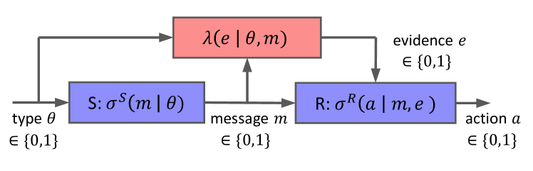
Figure 1: Signaling games with evidence add the red detector block to the $S$ and $R$ blocks. The probability $\lambda(e\,|\,\theta,m)$ of emitting evidence $e$ depends on $S$’s type $\theta$ and the message $m$ that she transmits.

II-A Types, Messages, Evidence, Actions, and Beliefs

Table I: Summary of Notation

Notation	Meaning
$S,\>R$	Sender and Receiver
$\theta\in\Theta,\>m\in M,\>a\in A$	Types, Messages, Actions
$u^{X}\left(\theta,m,a\right)$	Utility Functions of Player $X\in\left\{S,R\right\}$
$p\left(\theta\right)$	Prior Probability of $\theta$
$\sigma^{S}\left(m\,|\,\theta\right)$	Mixed Strategy of $S$ of Type $\theta$
$\lambda\left(e\,|\,\theta,m\right)$	Probability of $e$ for Type $\theta$ & Message $m$
$\sigma^{R}\left(a\,|\,m,e\right)$	Mixed Strategy of $R$ given $m,\,e$
$\mu^{R}\left(\theta\,|\,m,e\right)$	Belief of $R$ that $S$ is of Type $\theta$
$\bar{u}^{S}\left(\sigma^{S},\sigma^{R}\,|\,\theta\right)$	Expected Utility for $S$ of Type $\theta$
$\bar{u}^{R}\left(\sigma^{R}\,|\,\theta,m,e\right)$	Expected Utility for $R$ given $\theta,$ $m,$ $e$
$\alpha\in\left[0,1\right]$	“Size” of Detector (False Positive Rate)
$\beta\in$$\left[\alpha,1\right]$	“Power” of Detector (True Positive Rate)

We consider binary information and action spaces in order to simplify analysis. Table I summarizes the notation. Let $\theta\in\Theta=\{0,1\}$ denote the private information of $S.$ Signaling games refer to $\theta$ as a type. The type could represent e.g., whether the sender is a malicious or benign actor, whether she has one set of preferences over another, or whether a given event observable to $S$ but not to $R$ has occurred. The type is drawn from a probability distribution $p,$ where $\sum_{\theta\in\Theta}p\left(\theta\right)=1$ and $\forall\theta\in\Theta,$ $p(\theta)\geq 0.$

Based on $\theta$, $S$ chooses a message $m\in M=\left\{0,1\right\}.$ She may use mixed strategies, i.e., she may select each $m$ with some probability. Let $\sigma^{S}\in\Gamma^{S}$ denote the strategy of $S,$ such that $\sigma^{S}(m\,|\,\theta)$ gives the probability with which $S$ sends message $m$ given that she is of type $\theta.$ The space of strategies satisfies

$$\Gamma^{S}=\biggl{\{}\sigma^{S}\,|\,\forall\theta,\,\underset{m\in M}{\sum}\sigma^{S}\left(m\,|\,\theta\right)=1;\>\forall\theta,m,\;\sigma^{S}\left(m\,|\,\theta\right)\geq 0\biggr{\}}.$$

Since $\Theta$ and $M$ are identical, a natural interpretation of an honest message is $m=\theta,$ while a deceptive message is represented by $m\neq\theta.$

Next, the detector emits evidence based on whether the message $m$ is equal to the type $\theta.$ The detector emits $e\in E=\left\{0,1\right\}$ by the probability $\lambda\left(e\,|\,\theta,m\right).$ Let $e=1$ denote an alarm and $e=0$ no alarm. The probability with which a detector records a true positive is called the power $\beta\in[0,1]$ of the detector. For simplicity, we set both true-positive rates to be equal: $\beta=\lambda(1\,|\,0,1)=\lambda(1\,|\,1,0).$ Similarly, let $\alpha$ denote the size of the detector, which refers to the false-positive rate. We have $\alpha=\lambda(1\,|\,0,0)=\lambda(1\,|\,1,1).$ A valid detector has $\beta\geq\alpha.$ This is without loss of generality, because otherwise $\alpha$ and $\beta$ can be relabeled.

After receiving both $m$ and $e,$ $R$ chooses an action $a\in A=\left\{0,1\right\}.$ $R$ may also use mixed strategies. Let $\sigma^{R}\in\Gamma^{R}$ denote the strategy of $R$ such that his mixed-strategy probability of playing action $a$ given message $m$ and evidence $e$ is $\sigma^{R}(a\,|\,m,e).$ The space of strategies is $\Gamma^{R}=$

$$\Bigl{\{}\sigma^{R}\,|\,\forall m,e,\>\underset{a\in A}{\sum}\sigma^{R}\left(a\,|\,m,e\right)=1;\,\forall e,m,a,\;\sigma^{R}\left(a\,|\,m,e\right)\geq 0\Bigr{\}}.$$

Based on $m$ and $e,$ $R$ forms a belief about the type $\theta$ of $S.$ For all $\theta,$ $m,$ and $e,$ define $\mu^{R}:\,\Theta\to\left[0,1\right]$ such that $\mu^{R}(\theta\,|\,m,e)$ gives the likelihood with which $R$ believes that $S$ is of type $\theta$ given message $m$ and evidence $e.$ $R$ uses belief $\mu^{R}$ to decide which action to chose.

II-B Utility Functions

Let $u^{S}:\,\Theta\times M\times A\to\mathbb{R}$ denote a utility function for $S$ such that $u^{S}\left(\theta,m,a\right)$ gives the utility that she receives when her type is $\theta,$ she sends message $m,$ and $R$ plays action $a.$ Similarly, let $u^{R}:\,\Theta\times M\times A$ denote $R$’s utility function so that $u^{R}\left(\theta,m,a\right)$ gives his payoff under the same scenario.

Only a few assumptions are necessary to characterize a deceptive interaction. Assumption $1$ is that $u^{S}$ and $u^{R}$ do not depend (exogenously) on $m,$ i.e., the interaction is a cheap-talk game. Assumptions 2-3 state that $R$ receives higher utility if he correctly chooses $a=\theta$ than if he chooses $a\neq\theta.$ Formally,

$$u^{R}\left(0,m,0\right)>u^{R}\left(0,m,1\right),\;u^{R}\left(1,m,0\right)<u^{R}\left(1,m,1\right).$$

Finally, Assumptions 4-5 state that $S$ receives higher utility if $R$ chooses $a\neq\theta$ than if he chooses $a=\theta.$ That is,

$$u^{S}\left(0,m,0\right)<u^{S}\left(0,m,1\right),\;u^{S}\left(1,m,0\right)>u^{S}\left(1,m,1\right).$$

Together, Assumptions 1-5 characterize a cheap-talk signaling game with evidence.

Define an expected utility function $\bar{u}^{S}:\,\Gamma^{S}\times\Gamma^{R}\to\mathbb{R}$ such that $\bar{u}^{S}\left(\sigma^{S},\sigma^{R}\,|\,\theta\right)$ gives the expected utility to $S$ when she plays strategy $\sigma^{S},$ given that she is of type $\theta.$ This expected utility is given by

$$\bar{u}^{S}\left(\sigma^{S},\sigma^{R}\,|\,\theta\right)=\sum_{a\in A}\sum_{e\in E}\sum_{m\in M}\\ \sigma^{R}\left(a\,|\,m,e\right)\lambda\left(e\,|\,\theta,m\right)\sigma^{S}\left(m\,|\,\theta\right)u^{S}\left(\theta,m,a\right).$$

Next define $\bar{u}^{R}:\,\Gamma^{R}\to\mathbb{R}$ such that $\bar{u}^{R}(\sigma^{R}\,|\,\theta,m,e)$ gives the expected utility to $R$ when he plays strategy $\sigma^{R}$ given message $m,$ evidence $e,$ and sender type $\theta.$ The expected utility function is given by

$$\bar{u}^{R}(\sigma^{R}\,|\,\theta,m,e)=\sum_{a\in A}\sigma^{R}\left(a\,|\,m,e\right)u^{R}\left(\theta,m,a\right).$$

II-C Equilibrium Concept

In two-player games, Nash equilibrium defines a strategy profile in which each player best responds to the optimal strategies of the other player [19]. Signaling games motivate the extension of Nash equilibrium in two ways. First, information asymmetry requires $R$ to maximize his expected utility over the possible types of $S.$ An equilibrium in which $S$ and $R$ best respond to each other’s strategies given some belief $\mu^{R}$ is called a Bayesian Nash equilibrium [11]. We also require $R$ to update $\mu^{R}$ rationally. Perfect Bayesian Nash equilibrium (PBNE) captures this constraint. Definition 1 applies PBNE to our game.

Definition 1.

(Perfect Bayesian Nash Equilibrium [7]) A PBNE of a cheap-talk signaling game with evidence is a strategy profile $(\sigma^{S*},\sigma^{R*})$ and posterior beliefs $\mu^{R}(\theta\,|\,m,e)$ such that

$$\forall\theta\in\Theta,\>\sigma^{S*}\in\underset{\sigma^{S}\in\Gamma^{S}}{\arg\max}\,\bar{u}^{S}\left(\sigma^{S},\sigma^{R*}\,|\,\theta\right),$$ (1)

$\forall m\in M,\>\forall e\in E,$

$$\sigma^{R*}\in\underset{\sigma^{R}\in\Gamma^{R}}{\arg\max}\,\sum_{\theta\in\Theta}\mu^{R}\left(\theta\,|\,m,e\right)\bar{u}^{R}(\sigma^{R}\,|\,\theta,m,e),$$ (2)

and if $\underset{\tilde{\theta}\in\Theta}{\sum}\lambda(e\,|\,\tilde{\theta},m)\sigma^{S}(m\,|\,\tilde{\theta})p(\tilde{\theta})>0,$ then

$$\mu^{R}\left(\theta\,|\,m,e\right)=\frac{\lambda\left(e\,|\,\theta,m\right)\mu^{R}\left(\theta\,|\,m\right)}{\underset{\tilde{\theta}\in\Theta}{\sum}\lambda\left(e\,|\,\tilde{\theta},m\right)\mu^{R}\left(\tilde{\theta}\,|\,m\right)},$$ (3)

where

$$\mu^{R}\left(\theta\,|\,m\right)=\frac{\sigma^{S}\left(m\,|\,\theta\right)p\left(\theta\right)}{\underset{\hat{\theta}\in\Theta}{\sum}\sigma^{S}\left(m\,|\,\hat{\theta}\right)p\left(\hat{\theta}\right)}.$$ (4)

If $\underset{\tilde{\theta}\in\Theta}{\sum}\lambda(e\,|\,\tilde{\theta},m)\sigma^{S}(m\,|\,\tilde{\theta})p(\tilde{\theta})=0,$ then $\mu^{R}\left(\theta\,|\,m,e\right)$ may be set to any probability distribution over $\Theta.$

Equations (3)-(4) require the belief to be set according to Bayes’ Law. First, $R$ updates her belief according to $m$ using Eq. (4). Then $R$ updates her belief according to $e$ using Eq. (3). This step is not present in the traditional definition of PBNE for signaling games.

There are three categories of PBNE: separating, pooling, and partially-separating equilibria. These are defined based on the strategy of $S.$ In separating PBNE, the two types of $S$ transmit opposite messages. This allows $R$ to infer $S$’s type with certainty. In pooling PBNE, both types of $S$ send messages with identical probabilities. That is, $\forall m\in M,\>\sigma^{S}(m\,|\,0)=\sigma^{S}(m\,|\,1).$ This makes $m$ useless to $R.$ $R$ updates his belief based only on the evidence $e.$ Equations (3)-(4) yield

$$\mu^{R}\left(\theta\,|\,m,e\right)=\frac{\lambda\left(e\,|\,\theta,m\right)p\left(\theta\right)}{\underset{\tilde{\theta}\in\Theta}{\sum}\lambda\left(e\,|\,\tilde{\theta},m\right)p\left(\tilde{\theta}\right)}.$$ (5)

In partially-separating PBNE, the two types of $S$ transmit messages with different, but not completely opposite, probabilities. In other words, $\forall m\in M,$ $\sigma^{S}(m\,|\,0)\neq\sigma^{S}(m\,|\,1),$ and $\sigma^{S}(m\,|\,0)\neq 1-\sigma^{S}(m\,|\,1).$ Equations (3)-(4) allow $R$ to update his belief, but the belief remains uncertain.

III Equilibrium Results

In this section, we find the PBNE of the cheap-talk signaling game with evidence. We present the analysis in four steps. In Subsection III-A, we solve the optimality condition for $R,$ which determines the structure of the results. In Subsection III-B, we solve the optimality condition for $S,$ which determines the equilibrium beliefs $\mu^{R}.$ We present the pooling equilibria of the game in Subsection III-C. Some parameter regimes do not admit any pooling equilibria. For those regimes, we derive partially-separating equilibria in Subsection III-D.

First, Lemma 1 notes that one class of equilibria is not supported.

Lemma 1.

Under Assumptions 1-5, the game admits no separating PBNE.

The proof is straightforward, so we omit it here. Lemma 1 results from the opposing utility functions of $S$ and $R.$ $S$ wants to deceive $R,$ and $R$ wants to correctly guess the type. It is not incentive-compatible for $S$ to fully reveal the type by choosing a separating strategy.

III-A Prior Probability Regimes

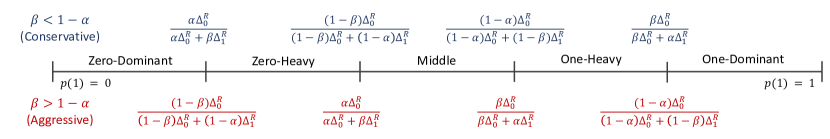
Figure 2: PBNE differ within five prior probability regimes. In the Zero-Dominant regime, $p(\theta=1)\approx 0,$ i.e., type $0$ dominates. In the Zero-Heavy regime, $p(\theta=1)$ is slightly higher, but still low. In the Middle regime, the types are mixed almost evenly. The One-Heavy regime has a higher $p(\theta=1),$ and the One-Dominant regime has $p(\theta=1)\approx 1.$ The definitions of the regime boundaries depend on whether the detector is conservative or aggressive.

Next, we look for pooling PBNE. Consider $R$’s optimal strategies $\sigma^{R*}$ in this equilibrium class. Note that if the sender uses a pooling strategy on message $m$ (i.e., if $S$ with both $\theta=0$ and $\theta=1$ send message $m$), then $\sigma^{R*}(1\,|\,m,e)$ gives $R$’s optimal action $a$ after observing evidence $e.$ Messages do not reveal anything about the type $\theta,$ and $R$ updates his belief using Eq. (5). For brevity, define the following notations:

$$\Delta_{0}^{R}\triangleq u^{R}\left(\theta=0,m,a=0\right)-u^{R}\left(\theta=0,m,a=1\right),$$ (6)

$$\Delta_{1}^{R}\triangleq u^{R}\left(\theta=1,m,a=1\right)-u^{R}\left(\theta=1,m,a=0\right).$$ (7)

$\Delta_{0}^{R}$ gives the benefit to $R$ for correctly guessing the type when $\theta=0,$ and $\Delta_{1}^{R}$ gives the benefit to $R$ for correctly guessing the type when $\theta=1.$ Since the game is a cheap-talk game, these benefits are independent of $m.$ Lemmas 2-3 solve for $\sigma^{R*}$ within five regimes of the prior probability $p(\theta)$ of each type $\theta\in\{0,1\}.$ Recall that $p(\theta)$ represents $R$’s belief that $S$ has type $\theta$ before $R$ observes $m$ or $e.$

Lemma 2.

For pooling PBNE, $R$’s optimal actions $\sigma^{R*}$ for evidence $e$ and messages $m$ on the equilibrium path vary within five regimes of $p(\theta).$ The top half of Fig. 2 lists the boundaries of these regimes for detectors in which $\beta<1-\alpha,$ and the bottom half of Fig. 2 lists the boundaries of these regimes for detectors in which $\beta>1-\alpha.$

Proof:

See Appendix A.∎

Remark 1.

Boundaries of the equilibrium regimes differ depending on the relationship between $\beta$ and $1-\alpha.$ $\beta$ is the true-positive rate and $1-\alpha$ is the true-negative rate. Let us call detectors with $\beta<1-\alpha$ conservative detectors, detectors with $\beta>1-\alpha$ aggressive detectors, and detectors with $\beta=1-\alpha$ equal-error-rate (EER) detectors. Aggressive detectors have high true-positive rates but also high false-positive rates. Conservative detectors have low false-positive rates but also low true-positive rates. Equal-error-rate detectors have an equal rate of false-positives and false-negatives.

Remark 2.

The regimes in Fig. 2 shift towards the right as $\Delta_{0}^{R}$ increases. Intuitively, a higher $p(1)$ is necessary to balance out the benefit to $R$ for correctly identifying a type $\theta=0$ as $\Delta_{0}^{R}$ increases. The regimes shift towards the left as $\Delta_{1}^{R}$ increases for the opposite reason.

Lemma 3 gives the optimal strategies of $R$ in response to pooling behavior within each of the five parameter regimes.

Lemma 3.

For each regime, $\sigma^{R*}$ on the equilibrium path is listed in Table III if $\beta<1-\alpha$ and in Table III if $\beta>1-\alpha.$ The row labels correspond to the Zero-Dominant (O-D), Zero-Heavy (0-H), Middle, One-Heavy (1-H), and One-Dominant (1-D) regimes.

Proof:

See Appendix A. ∎

Table II: $\sigma^{R*}(1\,|m,e)$ in Pooling PBNE with $\beta<1-\alpha$

	$\sigma^{R*}(1\,|\,0,0)$	$\sigma^{R*}(1\,|\,0,1)$	$\sigma^{R*}(1\,|\,1,0)$	$\sigma^{R*}(1\,|\,1,1)$
0-D	0	0	0	0
0-H	0	1	0	0
Middle	0	1	1	0
1-H	1	1	1	0
1-D	1	1	1	1

Table III: $\sigma^{R*}(1\,|m,e)$ in Pooling PBNE with $\beta>1-\alpha$

	$\sigma^{R*}(1\,|\,0,0)$	$\sigma^{R*}(1\,|\,0,1)$	$\sigma^{R*}(1\,|\,1,0)$	$\sigma^{R*}(1\,|\,1,1)$
0-D	0	0	0	0
0-H	0	0	1	0
Middle	0	1	1	0
1-H	0	1	1	1
1-D	1	1	1	1

Remark 3.

In the Zero-Dominant and One-Dominant regimes of all detector classes, $R$ determines $\sigma^{R*}$ based only on the overwhelming prior probability of one type over the other. In the Zero-Dominant regime, $R$ chooses $\sigma^{R*}(1\,|\,m,e)=0$ for all $m$ and $e,$ and in the One-Dominant regime, $R$ chooses $\sigma^{R*}(1\,|\,m,e)=1$ for all $m$ and $e.$

Remark 4.

In the Middle regime of both detector classes, $R$ chooses $\sigma^{R*}(1\,|\,m,0)=m$ and $\sigma^{R*}(1\,|\,m,1)=1-m.$ In other words, $R$ believes the message of $S$ if $e=0$ and does not believe the message of $S$ if $e=1.$

III-B Optimality Condition for $S$

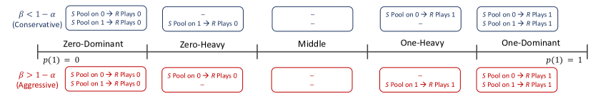
Figure 3: PBNE in each of the parameter regimes defined in Fig. 2. For $m\in\{0,1\},$ “$S$ Pool on $m$” signifies $\sigma^{S*}(m\,|\,0)=\sigma^{S*}(m\,|\,1)=1.$ For $a\in\{0,1\}$, “$R$ Plays $a$” signifies $\sigma^{R*}(a\,|\,0,0)=\sigma^{R*}(a\,|\,0,1)=\sigma^{R*}(a\,|\,1,0)=\sigma^{R*}(a\,|\,1,1)=1.$ Lemma 4 gives $\mu^{R}.$ The Dominant regimes support pooling PBNE on both messages. The Heavy regimes support pooling PBNE on only one message. The Middle regime does not support any pooling PBNE.

Next, we must check to see whether each possible pooling strategy is optimal for $S.$ This depends on what $R$ would do if $S$ were to deviate and send a message off the equilibrium path. $R$’s action in that case depends on his beliefs for messages off the path. In PBNE, these beliefs can be set arbitrarily. The challenge is to see whether beliefs $\mu^{R}$ exist such that each pooling strategy is optimal for both types of $S.$ Lemmas 4-5 give conditions under which such beliefs exist.

Lemma 4.

Let $m$ be the message on the equilibrium path. If $\sigma^{R*}(1\,|\,m,0)=\sigma^{R*}(1\,|\,m,1),$ then there exists a $\mu^{R}$ such that pooling on message $m$ is optimal for both types of $S.$ For brevity, let $a^{*}\triangleq\sigma^{R*}(1\,|\,m,0)=\sigma^{R*}(1\,|\,m,1).$ Then $\mu^{R}$ is given by,

$$\forall e\in E,\>\mu^{R}\left(\theta=a^{*}\,|\,1-m,e\right)\geq\frac{\Delta_{1-a^{*}}^{R}}{\Delta_{1-a^{*}}^{R}+\Delta_{a^{*}}^{R}}.$$

Lemma 5.

If $\sigma^{R*}(1\,|\,m,0)=1-\sigma^{R*}(1\,|\,m,1)$ and $\beta\neq 1-\alpha,$ then there does not exist a $\mu^{R}$ such that pooling on message $m$ is optimal for both types of $S.$

Proof:

See Appendix B for the proofs of Lemmas 4-5. ∎

The implications of these lemmas can be seen in the pooling PBNE results that are presented next.

III-C Pooling PBNE

Theorem 1 gives the pooling PBNE of the game.

Theorem 1.

(Pooling PBNE) The pooling PBNE are summarized by Fig. 3.

Proof:

The theorem results from combining Lemmas 2-5, which give the equilibrium $\sigma^{S*},$ $\sigma^{R*},$ and $\mu^{R}.$ ∎

Remark 5.

For $\beta<1-\alpha,$ the Zero-Heavy regime admits only a pooling PBNE on $m=1,$ and the One-Heavy regime admits only a pooling PBNE on $m=0.$ We call this situation (in which, typically, $m\neq\theta$) a falsification convention. (See Section IV.) For $\beta>1-\alpha,$ the Zero-Heavy regime admits only a pooling PBNE on $m=0,$ and the One-Heavy regime admits only a pooling PBNE on $m=1.$ We call this situation (in which, typically, $m=\theta$) a truth-telling convention.

Remark 6.

For $\beta\neq 1-\alpha,$ the Middle regime does not admit any pooling PBNE. This occurs because $R$’s responses to message $m$ depends on $e,$ i.e., $\sigma^{R*}(1\,|\,0,0)=1-\sigma^{R*}(1\,|\,0,1)$ and $\sigma^{R*}(1\,|\,1,0)=1-\sigma^{R*}(1\,|\,1,1).$ One of the types of $S$ prefers to deviate to the message off the equilibrium path. Intuitively, for a conservative detector, $S$ with type $\theta=m$ prefers to deviate to message $1-m,$ because his deception is unlikely to be detected. On the other hand, for an aggressive detector, $S$ with type $\theta=1-m$ prefers to deviate to message $1-m,$ because his honesty is likely to produce a false-positive alarm, which will lead $R$ to guess $a=m.$ Appendix B includes a formal derivation of this result.

III-D Partially-Separating PBNE

For $\beta\neq 1-\alpha,$ since the Middle regime does not support pooling PBNE, we search for partially-separating PBNE. In these PBNE, $S$ and $R$ play mixed strategies. In mixed-strategy equilibria in general, each player chooses a mixed strategy that makes the other players indifferent between the actions that they play with positive probability. Theorems 2-3 give the results.

Theorem 2.

(Partially-Separating PBNE for Conservative Detectors) For $\beta<1-\alpha,$ within the Middle Regime, there exists an equilibrium in which the sender strategies are

$$\sigma^{S*}\left(m=1\,|\,\theta=0\right)= \frac{\beta^{2}}{\beta^{2}-\alpha^{2}}-\frac{\alpha\beta\Delta_{1}^{R}}{\left(\beta^{2}-\alpha^{2}\right)\Delta_{0}^{R}}\left(\frac{p}{1-p}\right),$$

$$\sigma^{S*}\left(m=1\,|\,\theta=1\right)= \frac{\alpha\beta\Delta_{0}^{R}}{\left(\beta^{2}-\alpha^{2}\right)\Delta_{1}^{R}}\left(\frac{1-p}{p}\right)-\frac{\alpha^{2}}{\beta^{2}-\alpha^{2}},$$

the receiver strategies are

$$\sigma^{R*}(a=1\,|\,m=0,e=0)=\, \frac{1-\alpha-\beta}{2-\alpha-\beta},$$

$$\sigma^{R*}(a=1\,|\,m=0,e=1)=\, 1,$$

$$\sigma^{R*}(a=1\,|\,m=1,e=0)=\, \frac{1}{2-a-b},$$

$$\sigma^{R*}(a=1\,|\,m=1,e=1)=\, 0,$$

and the beliefs are computed by Bayes’ Law in all cases.

Theorem 3.

(Partially-Separating PBNE for Aggressive Detectors) For any $g\in[0,1],$ let $\bar{g}\triangleq 1-g.$ For $\beta>1-\alpha,$ within the Middle Regime, there exists an equilibrium in which the sender strategies are

$$\sigma^{S*}\left(m=1\,|\,\theta=0\right)= \frac{\bar{\alpha}\bar{\beta}\Delta_{1}^{R}}{\left(\bar{\alpha}^{2}-\bar{\beta}^{2}\right)\Delta_{0}^{R}}\left(\frac{p}{1-p}\right)-\frac{\bar{\beta}^{2}}{\bar{\alpha}^{2}-\bar{\beta}^{2}},$$

$$\sigma^{S*}\left(m=1\,|\,\theta=1\right)= \frac{\bar{\alpha}^{2}}{\bar{\alpha}^{2}-\bar{\beta}^{2}}-\frac{\bar{\alpha}\bar{\beta}\Delta_{0}^{R}}{\left(\bar{\alpha}^{2}-\bar{\beta}^{2}\right)\Delta_{1}^{R}}\left(\frac{1-p}{p}\right),$$

the receiver strategies are

$$\sigma^{R*}(a=1\,|\,m=0,e=0)=\, 0,$$

$$\sigma^{R*}(a=1\,|\,m=0,e=1)=\, \frac{1}{\alpha+\beta},$$

$$\sigma^{R*}(a=1\,|\,m=1,e=0)=\, 1,$$

$$\sigma^{R*}(a=1\,|\,m=1,e=1)=\, \frac{\alpha+\beta-1}{\alpha+\beta},$$

and the beliefs are computed by Bayes’ Law in all cases.

Proof:

See Appendix C for the proofs of Theorems 2-3. ∎

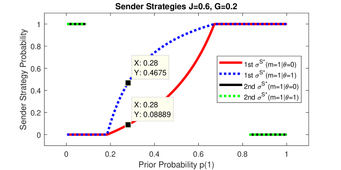
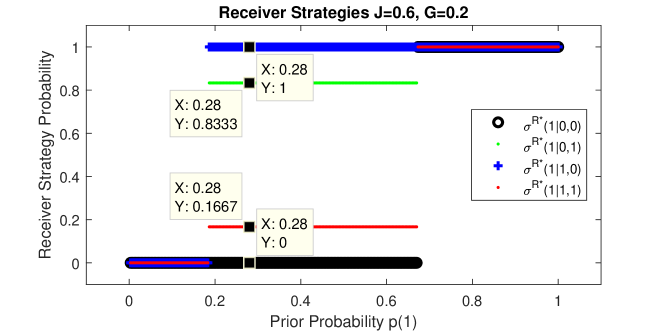
Figure 4: Equilibrium sender strategies for $\beta=0.9,$ $\alpha=0.3,$ $\Delta_{0}^{R}=15,$ and $\Delta_{1}^{R}=22.$ The Dominant regimes of $p(1)$ support both pooling on $m=0$ and $m=1.$ The Heavy regimes ($0.09<p<0.19$ and $0.67<p<0.83$) support only pooling on $m=0$ and $m=1,$ respectively. The Middle regime does not support any pooling PBNE, but does support a partially-separating PBNE.

Figure 5: Equilibrium receiver strategies for $\beta=0.9,$ $\alpha=0.3,$ $\Delta_{0}^{R}=15,$ and $\Delta_{1}^{R}=22.$ $R$ plays pure strategies in both the Dominant and Heavy regimes. In the Middle regime, two strategy components are pure, and two are mixed.

Remark 7.

In Theorem 2, $S$ chooses the $\sigma^{S*}$ that makes $R$ indifferent between $a=0$ and $a=1$ when he observes the pairs $(m=0,e=0)$ and $(m=1,e=0).$ This allows $R$ to choose mixed strategies for $\sigma^{R*}(1\,|\,0,0)$ and $\sigma^{R*}(1\,|\,1,0).$ Similarly, $R$ chooses $\sigma^{R*}(1\,|\,0,0)$ and $\sigma^{R*}(1\,|\,1,0)$ that make both types of $S$ indifferent between sending $m=0$ and $m=1.$ This allows $S$ to choose mixed strategies. A similar pattern follows in Theorem 3 for $\sigma^{S*},$ $\sigma^{R*}(1\,|\,0,1),$ and $\sigma^{R*}(1\,|\,1,1).$

Remark 8.

Note that none of the strategies are functions of the sender utility $u^{S}.$ As shown in Section IV, this gives the sender’s expected utility a surprising relationship with the properties of the detector.

Figure 5-5 depict the equilibrium strategies for $S$ and $R,$ respectively, for an aggressive detector. Note that the horizontal axis is the same as the horizontal axis in Fig. 2 and Fig. 3.

The Zero-Dominant and One-Dominant regimes feature two pooling equilibria. In Fig. 5, the sender strategies for the first equilibrium are depicted by the red and blue curves, and the sender strategies for the second equilibrium are depicted by the green and black curves. These are pure strategies, because they occur with probabilities of zero or one. The Zero-Heavy and One-Heavy regimes support only one pooling equilibria in each case.

The Middle regime of $p(1)$ features the partially-separating PBNE given in Theorem 3. In this regime, Fig. 5 shows that $R$ plays a pure strategy when $e=0$ and a mixed strategy when $e=1.$ The next section investigates the relationships between these equilibrium results and the parameters of the game.

IV Comparative Statics

In this section, we define quantities that we call the quality and aggressiveness of the detector. Then we define a quantity called truth-induction, and we examine the variation of truth-induction with the quality and aggressiveness of the detector.

IV-A Equilibrium Strategies versus Detector Characteristics

Consider an alternative parameterization of the detector by the pair $J$ and $G,$ where $J=\beta-\alpha\in[-1,1],$ and $G=\beta-\left(1-\alpha\right)\in[-1,1].$ $J$ is called Youden’s J Statistic [28]. Since an ideal detector has high $\beta$ and low $\alpha,$ $J$ parameterizes the quality of the detector. $G$ parameterizes the aggressiveness of the detector, since an aggressive detector has $\beta>1-\alpha$ and a conservative detector has $\beta<1-\alpha.$ Figure 6 depicts the transformation of the axes. Note that the pair $(J,G)$ fully specifies the pair $(\alpha,\beta).$

Figure 7 depicts the influences of $J$ and $G$ on $S$’s equilibrium strategy. The red (solid) curves give $\sigma^{S*}(m=1\,|\,\theta=0),$ and the blue (dashed) curves represent $\sigma^{S*}(m=1\,|\,\theta=1).$ Although the Zero-Dominant and One-Dominant regimes support two pooling equilibria, Fig. 7 only plots one pooling equilibrium for the sake of clarity.

In Column 1, $J$ is fixed and $G$ decreases from top to bottom. The top two plots have $G>0,$ and the bottom two have $G<0.$ There is a regime change at exactly $G=0.$ At that point, the equilibrium $\sigma^{S*}(1\,|\,0)$ and $\sigma^{S*}(1\,|\,1)$ flip to their complements. Here a small perturbation in the characteristics of the detector leads to a large change in the equilibrium strategies.

Column $2$ features a conservative detector: $G=-0.1.$ $J$ decreases from top to bottom. Note that a large $J$ leads to a large Middle regime, i.e., a large range of $p(1)$ for which $S$ plays mixed strategies in equilibrium. The detector in Column $3$ is aggressive: $G=0.1.$ Again, a large $J$ leads to a large Middle regime in which $S$ plays mixed strategies.

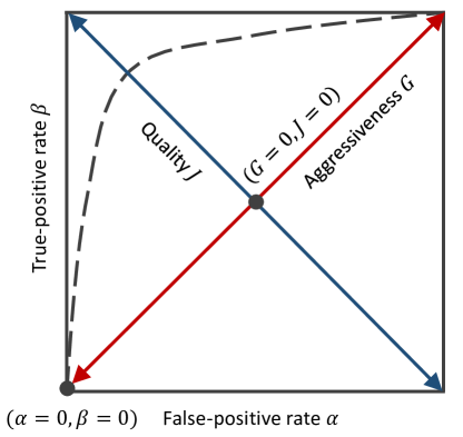
Figure 6: The detector characteristics can be plotted in ROC-space, with $\alpha$ on the horizontal axis and $\beta$ on the vertical axis. We also parameterize the detector characteristics by the orthogonal qualities $J\in[-1,1]$ and $G\in[-1,1].$ The dashed line gives a sample ROC-curve.

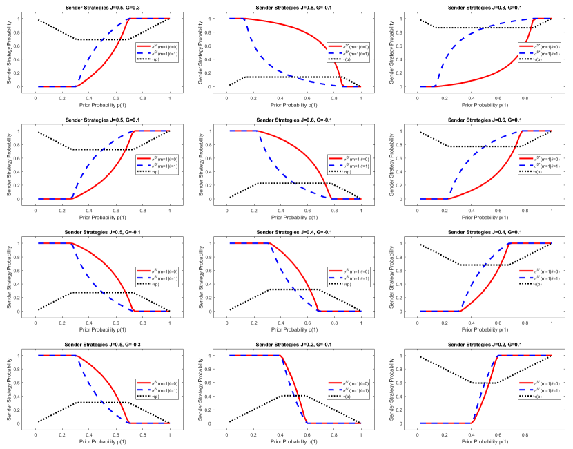
Figure 7: Sender equilibrium strategies $\sigma^{S*}$ and truth-induction rates $\tau.$ Column 1: Detector quality $J$ is fixed and aggressiveness $G$ decreases from top to bottom. Columns 2 and 3: $G$ is fixed and $J$ decreases from top to bottom. Column 2 is for a conservative detector, and Column 3 is for an aggressive detector. The sender equilibrium strategies are mixed within the Middle regime, and constant within the other regimes.

IV-B Truth-Induction

Consider the Middle regimes of the games plotted in Columns $2$ and $3.$ Note that in the Middle regime of Column $2,$ the probabilities with which both types of $S$ send $m=1$ decrease as $p(1)$ increases, while in the Middle regime of Column $3,$ the probabilities with which both types of $S$ send $m=1$ increases as $p(1)$ increases. This suggests that $S$ is somehow more “honest” for the aggressive detectors in Column $3,$ because $\theta$ and $m$ are more correlated for aggressive detectors than for conservative detectors.

In order to formalize this result, let $\sigma^{S*}(m\,|\,\theta;p)$ parameterize the sender’s equilibrium strategy by the prior probability $p\triangleq p(1).$ Then define a mapping $\tau:\,[-1,1]^{2}\times[0,1]\to[0,1],$ such that $\tau(J,G,p)$ gives the truth-induction rate of the detector parameterized by $(J,G)$ at the prior probability $p.$ We have

$$\tau\left(J,G,p\right)=\underset{\theta\in\{0,1\}}{\sum}\,p\sigma^{S*}\left(m=\theta\,|\,\theta;p\right).$$ (8)

The quantity $\tau$ gives the proportion of messages sent by $S$ for which $m=\theta,$ i.e., for which $S$ tells the truth. From this definition, we have Theorem 4.

Theorem 4.

(Detectors and Truth Induction Rates) Set $\Delta_{0}^{R}=\Delta_{1}^{R}.$ Then, within prior probability regimes that feature unique PBNE (i.e., the Zero-Heavy, Middle, and One-Heavy Regimes), for all $J\in[0,1]$ and $\forall p\in[0,1],$ we have that

$$\tau\left(J,G,p\right)\leq\frac{1}{2} \;\;\text{for}\;\;G\in\left(-1,0\right],$$

$$\tau\left(J,G,p\right)\geq\frac{1}{2} \;\;\text{for}\;\;G\in\left[0,1\right).$$

Proof:

See Appendix D.∎

Remark 9.

We can summarize Theorem 4 by stating that aggressive detectors induce a truth-telling convention, while conservative detectors induce a falsification convention.

The black curves in Fig. 7 plot $\tau(p)$ for each of the equilibrium strategies of $S.$ In the regimes with only one pair of equilibrium strategies for $S,$ $\tau(p)<1/2$ in Column $2$ and $\tau(p)>1/2$ in Column $3.$ In the Middle regime of Column $3,$ $\tau(p)$ is largest for detectors with high quality $J.$

IV-C Equilibrium Utility

The a priori expected equilibrium utilities of $S$ and $R$ are are the utilities that the players expect before $\theta$ is drawn. Denote these utilities by $\tilde{U}^{S}\in\mathbb{R}$ and $\tilde{U}^{R}\in\mathbb{R},$ respectively. For $X\in\{S,R\},$ the utilities are given by

$$\tilde{U}^{X}=\underset{\theta\in\Theta}{\sum}\,\underset{m\in M}{\sum}\,\underset{e\in E}{\sum}\,\underset{a\in A}{\sum}\,p\left(\theta\right)\\ \sigma^{S*}\left(m\,|\,\theta\right)\lambda\left(e\,|\,\theta,m\right)\sigma^{R*}\left(a\,|\,m,e\right)u^{X}\left(\theta,m,a\right).$$

Based on numerical experiments, we offer two propositions, leaving formal proofs for future work.

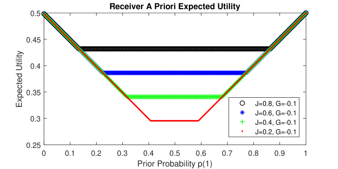
Figure 8: $R$’s a priori expected utility for varying $J.$ Towards the extremes of $p(1),$ $R$’s a priori expected utility does not depend on $J,$ because $R$ ignores $e.$ But in the middle regime, $R$’s expected utility increases with $J.$

Proposition 1.

Fix an aggressiveness $G.$ Then, for all $p\in[0,1],$ $\tilde{U}^{R}$ is monotonically non-decreasing in $J.$

Figure 8 illustrates Proposition 1. The proposition claims that $R$’s utility improves as detector quality improves. In the Middle regime of this example, $R$’s expected utility increases from $J=0.2$ to $J=0.8.$ Intuitively, as his detection ability improves, his belief $\mu^{R}$ becomes more certain. In the Zero-Dominant, Zero-Heavy, One-Heavy, and One-Dominant regimes, $R$’s equilibrium utility is not affected, because he ignores $e$ and chooses $a$ based only on prior probability.

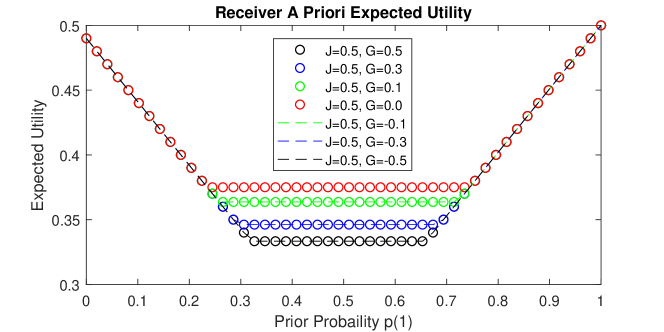
Figure 9: $R$’s a priori expected utility for varying $G.$ Towards the extremes of $p(1),$ $R$’s a priori expected utility does not depend on $G,$ because $R$ ignores $e.$ But in the middle regime, $R$’s expected utility decreases with $|G|.$

Proposition 2.

Fix a detector quality $J.$ Then, for all $p\in[0,1],$ $\tilde{U}^{R}$ is monotonically non-increasing in $|G|.$

For a fixed detector quality, Proposition 2 suggests that it is optimal for $R$ to use an EER detector. Figure 9 plots $R$’s expected a priori equilibrium utility for various $G$ given a fixed value of $J.$ In the example, the same color is used for each detector with aggressiveness $G$ and its opposite $-G.$ Detectors with $G\geq 0$ are plotted using circles, and detectors with $G<0$ are plotted using dashed lines. The utilities are the same for detectors with $G$ and $-G.$ In the Middle regime, expected utility increases as $|G|$ decreases from $0.5$ to $0.$

V Case Study

In this section, we apply signaling games with evidence to the use of defensive deception for network security. We illustrate the physical meanings of the action sets and equilibrium outcomes of the game for this application. We also present several results based on numerical experiments.

V-A Motivation

Traditional cybersecurity technologies such as firewalls, cryptography, and role-based access control (RBAC) are insufficient against new generations of sophisticated and well-resourced adversaries. Attackers capable of advanced persistent threats (APTs) use techniques such as social engineering and hardware exploits to circumvent defenses and gain insider access. Stealthy and evasive maneuvers are crucial elements of APTs. Often, attackers are able to remain within a network for several months or years before they are detected by network defenders [4]. This gives the attackers an advantage of information asymmetry.

To counteract this information asymmetry, defenders have developed various technologies that detect attackers and provide attackers with false information. In fact, honeypots are classical mechanisms that achieve both goals. Honeypots are systems placed within a network in such a manner that the systems are never accessed by legitimate users. Any activity on the honeypots is evidence that the network has been breached by an attacker. Sophisticated research honeypots run real services such as a file transfer protocol (FTP) server in order to allow interaction. In this way, the honeypots gather extensive information about the attacker’s techniques, tools, and procedures (TTP) [26].

To some extent, honeypots mimic production systems in order to appear attractive to attackers. One way of making honeypots appear attractive is to run programs that simulate user activity. This is a form of defensive deception. At the same time, attackers may be able to detect that a deceptive program is running. Hence, honeypot deployment is the detectable deception that can be captured by our model.

V-B Model Description

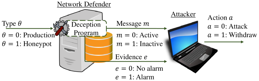
Figure 10: A defender adds either a production system or a honeypot to a network. Without any deception, the activity level of the system is $m=\theta.$ The defender can run a deception program in order to set $m=1-\theta,$ but the attacker can detect this program ($e=1$) with some probability. Then the defender decides whether to attack.

V-B1 Players and Types

Figure 10 casts the honeypot interaction as a signaling game with evidence. The players are the network defender (the sender, $S$) and the attacker (the receiver, $R$). The private information of the sender is the type of the system, $\theta\in\{0,1\},$ where $\theta=0$ represents a production system, and $\theta=1$ represents a honeypot.

V-B2 Messages

Typically, production systems have high activity (since they are accessed by real users) and honeypots have low activity (since they are not accessed by real users). Let $m=0$ denote that the system is active, and let $m=1$ denote that the system is inactive. In order to deceive $R,$ $S$ can manipulate the activity level of the system. For instance, with a honeypot, $S$ can send packets from some other source to the honeypot, create a program to simulate mouse movement on the honeypot, and create icons on the desktop. All of these make the honeypot appear active: $m=0.$ Similarly, with a production system, $S$ can write programs or create user policies that decrease incoming traffic or limit mouse movement and the number of visible desktop icons. All of these make the production system appear to be inactive: $m=1.$

V-B3 Evidence

With some probability, $R$ can detect the use of programs that manipulate the activity level of the system. For instance, if $S$ makes a honeypot ($\theta=1$) appear active ($m=0$), $R$ may observe that incoming traffic comes from a single automated source rather than from multiple human sources. He may also observe that simulated mouse movement follows patterns different from normal mouse movement, or that desktop icons are never used. These constitute an alarm: $e=1.$ If $R$ does not notice these suspicious signals, then there is no alarm: $e=0.$ Similarly, if $S$ creates programs or user policies for a production system ($\theta=0$) that limit the incoming traffic and user activity ($m=1$), $R$ may observe evidence that user behaviors are being artificially manipulated, which constitutes an alarm: $e=1.$ If $R$ does not notice this manipulation, then there is no alarm: $e=0.$

V-B4 Actions

After observing the activity level $m$ and leaked evidence $e,$ $R$ chooses an action $a\in\{0,1\}.$ Let $a=0$ denote attack, and let $a=1$ denote withdraw. Notice that $R$ prefers to choose $a=\theta,$ while $S$ prefers that $R$ choose $a\neq\theta.$ Hence, Assumptions 2-5 are satisfied. If the cost of running the deceptive program is negligible, then Assumption 1 is also satisfied.

V-C Equilibrium Results

We set the utility functions according to [3, 22]. Consider a detector with a true-positive rate $\beta=0.9$ and a false-positive rate $\alpha=0.3.$ This detector has $\beta>1-\alpha,$ so it is an aggressive detector, and the boundaries of the equilibrium regimes are given in the bottom half of Fig. 2. For this application, the Zero-Dominant and Zero-Heavy regimes can be called the Production-Dominant and Production-Heavy regimes, since type $\theta=0$ represents a production system. Similarly, the One-Heavy and One-Dominant regimes can be called the Honeypot-Heavy and Honeypot-Dominant regimes.

We have plotted the equilibrium strategies for these parameters in Fig. 5-5 in Section III. In the Production-Dominant regime ($p(\theta=1)<0.09$), there are very few honeypots. In equilibrium, $S$ can set both types of systems to a high activity level ($m=0$) or set both types of systems to a low activity level ($m=1$). In both cases, regardless of the evidence $e,$ $R$ attacks. Next, for the Production-Heavy regime ($0.09<p(1)<0.19$), the only equilibrium strategy for $S$ is a pooling strategy in which she leaves production systems ($\theta=0$) active ($m=0$) and runs a program on honeypots ($\theta=1$) in order to make them appear active ($m=1$) as well. $R$ is able to detect ($e=1$) the deceptive program on honeypots with probability $\beta=0.9,$ yet the prior probability $p(1)$ is low enough that it is optimal for $R$ to ignore the evidence and attack ($a=1$).

The Middle regime covers prior probabilities $0.19<p(1)<0.67.$ The figures display the players’ mixed strategies at $p(1)=0.28.$ For honeypots, $S$’s optimal strategy is to leave the activity level low with approximately $50\%$ probability ($\sigma^{S*}(1\,|\,1)\approx 0.47$) and to simulate a high activity level with approximately $50\%$ probability. For production systems, $S$’s optimal strategy is to decrease the activity level with a low probability ($\sigma^{S*}(1\,|\,0)\approx 0.09$) and to leave the activity level high with the remaining probability.

In the Middle regime, the receiver plays according to the activity level—i.e., trusts $S$’s message—if $e=0.$ If $e=1$ when $m=0,$ then most of the time, $R$ does not trust $S$ ($\sigma^{R*}(1\,|\,0,1)\approx 0.83$). Similarly, if $e=1$ when $m=1,$ then most of the time, $R$ does not trust $S$ ($\sigma^{R*}(1\,|\,1,1)\approx 0.17$). The pattern of equilibria in the Honeypot-Heavy and Honeypot-Dominant regimes is similar to the pattern of equilibria in the Production-Heavy and Production-Dominant regimes.

V-D Numerical Experiments and Insights

V-D1 Equilibrium Utility of the Sender

Next, Corollary 1 considers the relationship between $S$’s a priori equilibrium utility and the quality $J$ of the detector.

Corollary 1.

Fix an aggressiveness $G$ and prior probability $p(1).$ $S$’s a priori expected utility $\tilde{U}^{S}$ is not necessarily a decreasing function of the detector quality $J.$

Proof:

Figure 12 provides a counter-example. ∎

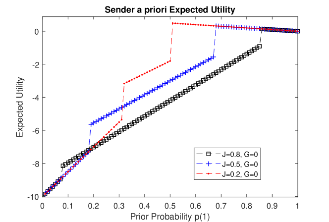
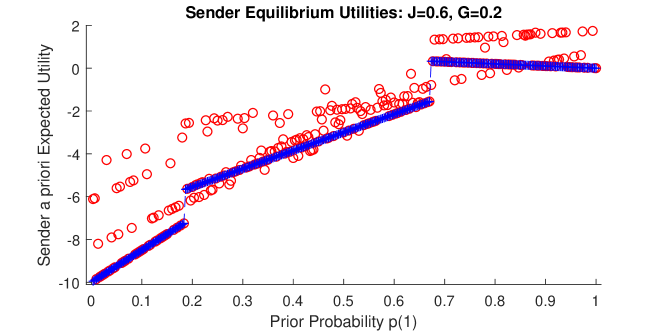
Figure 11: $S$’s a priori expected utility for varying $J.$ From least accurate detector to most accurate detector, the curves are colored red, blue, and black. Suprisingly, for some $p,$ $S$ does better with more accurate detectors than with less accurate detectors.

Figure 12: $S$’s a priori expected utility for playing her equilibrium strategy against 1) $R$’s equilibrium strategy (in blue crosses), and 2) sub-optimal strategies of $R$ (in red circles). Deviations from $R$’s equilibrium strategy almost always increase the expected utility of $S.$

Corollary 1 is counter-intuitive, because it seems that the player who attempts deception ($S$) should prefer poor deception detectors. Surprisingly, this is not always the case. Figure 12 displays the equilibrium utility for $S$ in the honeypot example for three different $J.$ At $p(1)=0.4,$ $S$ receives the highest expected utility for the lowest quality deception detector. But at $p(1)=0.1,$ $S$ receives the highest expected utility for the highest quality deception detector. In general, this is possible because the equilibrium regimes and strategies (e.g., in Theorems 1-3) depend on the utility parameters of $R,$ not $S.$

In particular, this occurs because of an asymmetry between the types. $S$ does very poorly if for a production system ($\theta=0$), she fails to deceive $R,$ so $R$ attacks ($a=0$). On the other hand, $S$ does not do very poorly if for a honeypot ($\theta=1$), she fails to deceive $R,$ who simply withdraws ($a=1$).

V-D2 Robustness of the Equilibrium Strategies

Finally, we investigate the performance of these strategies against sub-optimal strategies of the other player. Figure 12 shows the expected utility for $S$ when $R$ acts optimally in blue, and the expected utility for $S$ when $R$ occasionally acts sub-optimally in red. In almost all cases, $S$ earns higher expected utility if $R$ plays sub-optimally than if $R$ plays optimally.

It can also be shown that $R$’s strategy is robust against a sub-optimal $S.$ In fact, $R$’s equilibrium utility remains exactly the same if $S$ plays sub-optimally.

Corollary 2.

For all $\sigma^{S}\in\Gamma^{S},$ the a priori expected utility of $R$ for a fixed $\sigma^{R*}$ does not vary with $\sigma^{S}.$

Proof:

See Appendix E. ∎

Corollary 2 states that $R$’s equilibrium utility is not affected at all by deviations in the strategy of $S.$ This is a result of the structure of the partially-separating equilibrium. It suggests that $R$’s equilibrium strategy performs well even if $S$ is not fully rational.

VI Discussion

We have proposed a holistic and quantitative model of detectable deception called signaling games with evidence. The detector mechanism can be conceptualized in two ways. It can be seen as a technology that the receiver uses to detect deception. For instance, technology for a GPS receiver can detect spoofed position data based on a lack of variance in the carrier phase of the signal [24]. Alternatively, the detector can be seen as the inherent tendency of the information sender to emit cues during deceptive behavior. One example of this can be found in deceptive opinion spam in online marketplaces; fake reviews in these marketplaces tend to lack sensorial and concrete language such as spatial information [20]. Of course, both viewpoints are complementary, because cues of deceptive behavior are necessary in order for technology to be able to detect deception.

Our equilibrium results include a regime in which the receiver should chose whether to trust the sender based on the detector evidence (i.e., the Middle regime), and regimes in which the receiver should ignore the message and evidence and guess the private information using only the prior probabilities (the Zero-Dominant, Zero-Heavy, One-Heavy, and One-Dominant regimes). For the sender, our results indicate that it is optimal to partially reveal the private information in the former regime, while pooling behavior is optimal in the latter regimes. The analytical bounds that we have obtained on these regimes can be used to implement policies online, since they do not require iterative numerical computation.

We have also presented several contributions that are relevant for mechanism design. For instance, the mechanism designer can maximize the receiver utility by choosing an EER detector. Practically, designing the detector involves setting a threshold within a continuous space in order to classify an observation as an “Alarm” or “No Alarm.” For an EER detector, the designer chooses a threshold that obtains equal false-positive and false-negative error rates.

At the same time, we have shown that aggressive detectors induce a truth-telling convention, while conservative detectors of the same quality induce a falsification convention. This is important if truthful communication is considered to be a design objective in itself. One area in which this applies is trust management. In both human and autonomous behavior, an agent is trustworthy if it is open and honest, if “its capabilities and limitations [are] made clear; its style and content of interactions [do] not misleadingly suggest that it is competent where it is really not” [13]. Well-designed detectors can incentivize such truthful revelation of private information.

Additionally, even deceivers occasionally prefer to reveal some true information. Our numerical results have shown that the deceiver (the sender) sometimes receives a higher utility for a high quality detector than for a low quality detector. This result suggests that cybersecurity techniques that use defensive deception should not always strive to eliminate leakage. Sometimes, revealing cues to deception serves as a deterrent. Finally, the strategies of the sender and receiver are robust to non-equilibrium actions by the other player. This emerges from the strong misalignment between their objectives.

Future work could focus on the application of signaling games with evidence to specific technical domains. These domains often require adaptations of the model. For instance, problems with continuous type and message spaces can be addressed by applying a filter that maps the types and messages into binary spaces (c.f., Section VI of [23]). Computational methods can also be used to address large, discrete action spaces. Finally, signaling games with evidence can be embedded within larger frameworks in order to study deception in cyber-physical systems or deception across multiple links in a network. The present work provides theoretical foundations and fundamental insights that serve as a foundation for these further developments.

Appendix A Optimal Actions of $R$ in Pooling PBNE

Consider the case in which both types of $S$ send $m=0.$ On the equilibrium path, Eq. (5) yields $\mu^{R}(0\,|\,0,0)=(1-\alpha)p(0)/((1-\alpha)p(0)+(1-\beta)p(1))$ and $\mu^{R}(0\,|\,0,1)=\alpha p(0)/(\alpha p(0)+\beta p(1)),$ while off the equilibrium path, the beliefs can be set arbitrarily. From Eq. (2), $R$ chooses action $a=0$ (e.g., $R$ believes the signal of $S$) when evidence $e=0$ and $p(0)\geq\Delta_{1}^{R}(1-\beta)/(\Delta_{0}^{R}(1-\alpha)+\Delta_{1}^{R}(1-\beta)),$ or when evidence $e=1$ and $p(0)\geq\Delta_{1}^{R}\beta/(\Delta_{0}^{R}\alpha+\Delta_{1}^{R}\beta).$

Next, consider the case in which both types of $S$ send $m=1.$ Equation (5) yields $\mu^{R}(0\,|\,1,0)=(1-\beta)p(0)/((1-\beta)p(0)+(1-\alpha)p(1))$ and $\mu^{R}(0\,|\,1,1)=\beta p(0)/(\beta p(0)+\alpha p(1)),$ which leads $R$ to choose action $a=1$ (e.g. to believe the signal of $S$) if $e=0$ and $p(0)\leq\Delta_{1}^{R}(1-\alpha)/(\Delta_{0}^{R}(1-\beta)+\Delta_{1}^{R}(1-\alpha)),$ or if $e=1$ and $p(0)\leq\Delta_{1}^{R}\alpha/(\Delta_{0}^{R}\beta+\Delta_{1}^{R}\alpha).$ The order of these probabilities depends on whether $\beta>1-\alpha.$

Appendix B Optimal Actions of $S$ in Pooling PBNE

Let $S$ pool on a message $m.$ Consider the case that $\sigma^{R*}(1\,|\,m,0)=\sigma^{R*}(1\,|\,m,1),$ and let $a^{*}\triangleq\sigma^{R*}(1\,|\,m,0)=\sigma^{R*}(1\,|\,m,1).$ Then $S$ of type $\theta=1-a^{*}$ always successfully deceives $R.$ Clearly, that type of $S$ does not have an incentive to deviate. But type $S$ of type $\theta=a^{*}$ never deceives $R.$ We must set the off-equilibrium beliefs such that $S$ of type $\theta=a^{*}$ also would not deceive $R$ if she were to deviate to the other message. This is the case if $\forall e\in E,$ $\mu^{R}(a^{*}\,|\,1-m,e)\geq\Delta_{1-a^{*}}^{R}/(\Delta_{1-a^{*}}^{R}+\Delta_{a^{*}}^{R}).$ In that case, both types of $S$ meet their optimality conditions, and we have a pooling PBNE.

But consider the case if $\sigma^{R*}(1\,|\,m,0)=1-\sigma^{R*}(1\,|\,m,1),$ (i.e., if $R$’s response depends on evidence $e$). On the equilibrium path, $S$ of type $m$ receives utility

$$u^{S}\left(m,m,m\right)\left(1-\alpha\right)+u^{S}\left(m,m,1-m\right)\alpha,$$ (9)

and $S$ of type $1-m$ receives utility

$$u^{S}\left(1-m,m,1-m\right)\beta+u^{S}\left(1-m,m,m\right)\left(1-\beta\right).$$ (10)

Now we consider $R$’s possible response to messages off the equilibrium path.

First, there cannot be a PBNE if $R$ were to play the same action with both $e=0$ and $e=1$ off the equilibrium path. In that case, one of the $S$ types could guarantee deception by deviating to message $1-m.$ Second, there cannot be a PBNE if $R$ were to play action $a=m$ in response to message $1-m$ with evidence $0$ but action $a=1-m$ in response to message $1-m$ with evidence $1.$ It can be shown that both types of $S$ would deviate. The third possibility is that $R$ plays action $a=1-m$ in response to message $1-m$ if $e=0$ but action $a=m$ in response to message $1-m$ if $e=1.$ In that case, for deviating to message $1-m,$ $S$ of type $m$ would receive utility

$$u^{S}\left(m,1-m,m\right)\beta+u^{S}\left(m,1-m,1-m\right)\left(1-\beta\right),$$ (11)

and $S$ of type $1-m$ would receive utility

$$u^{S}\left(1-m,1-m,1-m\right)\left(1-\alpha\right)\\ +u^{S}\left(1-m,1-m,m\right)\alpha.$$ (12)

Combining Eq. (9-11), $S$ of type $m$ has an incentive to deviate if $\beta<1-\alpha.$ On the other hand, combining Eq. (10-12), $S$ of type $1-m$ has an incentive to deviate if $\beta>1-\alpha.$ Therefore, if $\beta\neq 1-\alpha,$ one type of $S$ always has an incentive to deviate, and a pooling PBNE is not supported.

Appendix C Derivation of Partially-Separating Equilibria

For brevity, define the notation $q\triangleq\sigma^{S*}(1\,|\,0),$ $r\triangleq\sigma^{S*}(1\,|\,1),$ $w\triangleq\sigma^{R*}(1\,|\,0,0),$ $x\triangleq\sigma^{R*}(1\,|\,0,1),$ $y\triangleq\sigma^{R*}(1\,|\,1,0),$ $z\triangleq\sigma^{R*}(1\,|\,1,1),$ and $K\triangleq\Delta_{1}^{R}/(\Delta_{0}^{R}+\Delta_{1}^{R}).$

We prove Theorem 2. First, assume the receiver’s pure strategies $x=1$ and $z=0.$ Second, $R$ must choose $w$ and $y$ to make both types of $S$ indifferent. This requires

$$\left[\begin{array}[]{cc}\bar{\alpha}&-\bar{\beta}\\ \bar{\beta}&-\bar{\alpha}\end{array}\right]\left[\begin{array}[]{c}w\\ y\end{array}\right]=\left[\begin{array}[]{c}-\alpha\\ -\beta\end{array}\right],$$

where $w,y\in[0,1].$ Valid solutions require $\beta\leq 1-\alpha.$

Third, $S$ must choose $q$ and $r$ to make $R$ indifferent for $(m,e)=(0,0)$ and $(m,e)=(1,0),$ which are the pairs that pertain to the strategies $w$ and $y.$ $S$ must satisfy

$$\left[\begin{array}[]{cc}-\bar{\alpha}\bar{p}\bar{K}&\bar{\beta}pK\\ -\bar{\beta}\bar{p}\bar{K}&\bar{\alpha}pK\end{array}\right]\left[\begin{array}[]{c}q\\ r\end{array}\right]=\left[\begin{array}[]{c}-\bar{\alpha}\bar{p}\bar{K}+\bar{\beta}pK\\ 0\end{array}\right].$$

Valid solutions require $p$ to be within the Middle regime for $\beta\leq 1-\alpha.$

Fourth, we must verify that the pure strategies $x=1$ and $z=0$ are optimal. This requires

$$\frac{\alpha\bar{r}p}{\alpha\bar{r}p+\beta\bar{q}\bar{p}}\leq\bar{K}\leq\frac{\beta rp}{\beta rp+\alpha q\bar{p}}.$$

It can be shown that, after substitution for $q$ and $r,$ this always holds. Fifth, the beliefs must be set everywhere according to Bayes’ Law. We have proved Theorem 2.

Now we prove Theorem 3. First, assume the receiver’s pure strategies $w=0$ and $y=1.$ Second, $R$ must choose $x$ and $z$ to make both types of $S$ indifferent. This requires

$$\left[\begin{array}[]{cc}\alpha&-\beta\\ \beta&-\alpha\end{array}\right]\left[\begin{array}[]{c}x\\ z\end{array}\right]=\left[\begin{array}[]{c}\bar{\beta}\\ \bar{\alpha}\end{array}\right],$$

where $x,y\in[0,1].$ Valid solutions require $\beta\geq 1-\alpha.$

Third, $S$ must choose $q$ and $r$ to make $R$ indifferent for $(m,e)=(0,1)$ and $(m,e)=(1,1),$ which are the pairs that pertain to the strategies $x$ and $z.$ $S$ must satisfy

$$\left[\begin{array}[]{cc}-\alpha\bar{p}\bar{K}&\beta pK\\ -\beta\bar{p}\bar{K}&\alpha pK\end{array}\right]\left[\begin{array}[]{c}q\\ r\end{array}\right]=\left[\begin{array}[]{c}-\alpha\bar{p}\bar{K}+\beta pK\\ 0\end{array}\right].$$

Valid solutions require $p$ to be within the Middle regime for $\beta\geq 1-\alpha.$

Fourth, we must verify that the pure strategies $w=0$ and $y=1$ are optimal. This requires

$$\frac{\alpha\bar{r}p}{\alpha\bar{r}p+\beta\bar{q}\bar{p}}\leq\bar{K}\leq\frac{\beta rp}{\beta rp+\alpha q\bar{p}}.$$

It can be shown that, after substitution for $q$ and $r,$ this always holds. Fifth, the beliefs must be set everywhere according to Bayes’ Law. We have proved Theorem 3.

Appendix D Truth-Induction Proof

We prove the theorem in two steps: first for the Middle regime and second for the Zero-Heavy and One-Heavy regimes.

For conservative detectors in the Middle regime, substituting the equations of Theorem 2 into Eq. (8) gives

$$\tau\left(J,G,p\right)=\frac{\bar{\alpha}\bar{\beta}-\bar{\beta}^{2}}{\bar{\alpha}^{2}-\bar{\beta}^{2}}=\frac{1}{2}\left(1-\frac{J}{1-G}\right)\leq\frac{1}{2}.$$

For aggressive detectors in the Middle regime, substituting the equations of Theorem 3 into Eq. (8) gives

$$\tau\left(J,G,p\right)=\frac{\beta^{2}-\alpha\beta}{\beta^{2}-\alpha^{2}}=\frac{1}{2}\left(1+\frac{J}{1+G}\right)\geq\frac{1}{2}.$$

This proves the theorem for the Middle regime.

Now we prove the theorem for the Zero-Heavy and One-Heavy regimes. Since $\Delta_{0}^{R}=\Delta_{1}^{R},$ all of the Zero-Heavy regime has $p(1)\leq 1/2,$ and all of the One-Heavy regime has $p(1)\geq 1/2.$ For conservative detectors in the Zero-Heavy regime, both types of $S$ transmit $m=1.$ $S$ of type $\theta=0$ are lying, while type $\theta=1$ are telling the truth. Since $p(1)\leq 1/2,$ we have $\tau\leq 1/2.$ Similarly, in the One-Heavy regime, both types of $S$ transmit $m=0.$ $S$ of type $\theta=0$ are telling the truth, while $S$ of type $\theta=1$ are lying. Since $p(1)\geq 1/2,$ we have $\tau\leq 1/2.$ On the other hand, for aggressive detectors, both types of $S$ transmit $m=0$ in the Zero-Heavy regime and $m=1$ in the One-Heavy regime. This yields $\tau\geq 1/2$ in both cases. This proves the theorem for the Zero-Heavy and One-Heavy regimes.

Appendix E Robustness Proof

Corollary 2 is obvious in the pooling regimes. In those regimes, $\sigma^{R*}(1\,|\,m,e)$ has the same value for all $m\in M$ and $e\in E$, so if $S$ plays the message off the equilibrium path, then there is no change in $R$’s action. In the mixed strategy regimes, using the expressions for $\sigma^{R*}$ from Theorems 2-3, it can be shown that, $\forall\theta\in\Theta,$ $m\in M,$ $a\in A,$

$$\underset{e\in E}{\sum}\,\lambda\left(e\,|\,\theta,m\right)\sigma^{R*}\left(a\,|\,m,0\right)=\\ \underset{e\in E}{\sum}\,\lambda\left(e\,|\,\theta,1-m\right)\sigma^{R*}\left(a\,|\,1-m,0\right).$$

In other words, for both types of $S,$ choosing either message results in the same probability that $R$ plays each actions. Since $u^{R}$ does not depend on $m,$ both messages result in the same utility for $R.$

References

- [1] Luigi Atzori, Antonio Iera, and Giacomo Morabito. The Internet of things: A survey. Comput. Networks, 54(15):2787–2805, 2010.
- [2] Rudolf Avenhaus, Bernhard Von Stengel, and Shmuel Zamir. Inspection games. Handbook of Game Theory with Econ. Applications, 3:1947–1987, 2002.
- [3] Thomas E Carroll and Daniel Grosu. A game theoretic investigation of deception in network security. Security and Commun. Nets., 4(10):1162–1172, 2011.
- [4] Ping Chen, Lieven Desmet, and Christophe Huygens. A study on advanced persistent threats. In IFIP Intl. Conf. on Communications and Multimedia Security, pages 63–72. Springer, 2014.
- [5] Hugh Cott. Adaptive Coloration in Animals. Methuen, 1940.
- [6] Vincent P Crawford and Joel Sobel. Strategic information transmission. Econometrica: J. of the Econometric Soc., pages 1431–1451, 1982.
- [7] Drew Fudenberg and Jean Tirole. Game Theory. The MIT Press, 1991.
- [8] Uri Gneezy. Deception: The role of consequences. American Econ. Review, 95(1):384–394, 2005.
- [9] Sanford J Grossman. The informational role of warranties and private disclosure about product quality. J. of Law and Econ., 24(3):461–483, 1981.
- [10] Sanford J Grossman and Oliver D Hart. Disclosure laws and takeover bids. J. of Finance, 35(2):323–334, 1980.
- [11] John C Harsanyi. Games with incomplete information played by “Bayesian” players. Manage. Sci., 50(12):1804–1817, 1967.
- [12] Lech J. Janczewski and Andrew M. Colarik. Cyber Warfare and Cyber Terrorism. Inform. Sci. Reference, New York, 2008.
- [13] Patricia M Jones and Christine M Mitchell. Human-computer cooperative problem solving: Theory, design, and evaluation of an intelligent associate system. IEEE Trans. on Systems, Man, and Cybernetics, 25(7):1039–1053, 1995.
- [14] Navin Kartik. Strategic communication with lying costs. Review of Economic Studies, 76(4):1359–1395, 2009.
- [15] Bernard C Levy. Binary and m-ary hypothesis testing. In Principles of Signal Detection and Parameter Estimation. Springer Science & Business Media, 2008.
- [16] James Edwin Mahon. The definition of lying and deception. In Edward N. Zalta, editor, Stanford Encyclopedia of Philosophy. Winter 2016 edition, 2016.
- [17] Paul R Milgrom. Good news and bad news: Representation theorems and applications. Bell J. of Econ., pages 380–391, 1981.
- [18] Umar Farooq Minhas, Jie Zhang, Thomas Tran, and Robin Cohen. A multifaceted approach to modeling agent trust for effective communication in the application of mobile ad hoc vehicular networks. IEEE Trans. Systems, Man, and Cybernetics, Part C (Applications and Reviews), 41(3):407–420, 2011.
- [19] John F Nash. Equilibrium points in n-person games. Proc. Nat. Acad. Sci. USA, 36(1):48–49, 1950.
- [20] Myle Ott, Yejin Choi, Claire Cardie, and Jeffrey T Hancock. Finding deceptive opinion spam by any stretch of the imagination. In Proc. 49th Annual Meeting Assoc. for Computational Linguistics: Human Language Technologies, pages 309–319, 2011.
- [21] Jeffrey Pawlick, Sadegh Farhang, and Quanyan Zhu. Flip the cloud: Cyber-physical signaling games in the presence of advanced persistent threats. In Decision and Game Theory for Security, pages 289–308. Springer, 2015.
- [22] Jeffrey Pawlick and Quanyan Zhu. Deception by design: Evidence-based signaling games for network defense. In Workshop on the Econ. of Inform. Security, Delft, The Netherlands, 2015.
- [23] Jeffrey Pawlick and Quanyan Zhu. Strategic trust in cloud-enabled cyber-physical systems with an application to glucose control. IEEE Trans. Inform. Forensics and Security, 12(12), 2017.
- [24] Mark L Psiaki, Todd E Humphreys, and Brian Stauffer. Attackers can spoof navigation signals without our knowledge. Here’s how to fight back GPS lies. IEEE Spectrum, 53(8):26–53, 2016.
- [25] Craig Silverman. This analysis shows how viral fake election news stories outperformed real news on facebook. BuzzFeed News, [Online]. Available: https://www.buzzfeed.com/craigsilverman/.
- [26] Lance Spitzner. The honeynet project: Trapping the hackers. IEEE Security & Privacy, 99(2):15–23, 2003.
- [27] Aldert Vrij, Samantha A Mann, Ronald P Fisher, Sharon Leal, Rebecca Milne, and Ray Bull. Increasing cognitive load to facilitate lie detection: The benefit of recalling an event in reverse order. Law and Human Behavior, 32(3):253–265, 2008.
- [28] William J Youden. Index for rating diagnostic tests. Cancer, 3(1):32–35, 1950.
- [29] Nan Zhang, Wei Yu, Xinwen Fu, and Sajal K Das. gPath: A game-theoretic path selection algorithm to protect tor’s anonymity. In Decision and Game Theory for Security, pages 58–71. Springer, 2010.
- [30] Quanyan Zhu and Tamer Başar. Game-theoretic approach to feedback-driven multi-stage moving target defense. In Decision and Game Theory for Security, pages 246–263. Springer, 2013.
- [31] J. Zhuang, V. M. Bier, and O. Alagoz. Modeling secrecy and deception in a multiple-period attacker–defender signaling game. European J. of Operational Res., 203(2):409–418, 2010.