NTUA-SLP at SemEval-2018 Task 1: Predicting Affective Content in Tweets with Deep Attentive RNNs and Transfer Learning

Abstract

In this paper we present deep-learning models that submitted to the SemEval-2018 Task 1 competition: “Affect in Tweets”. We participated in all subtasks for English tweets. We propose a Bi-LSTM architecture equipped with a multi-layer self attention mechanism. The attention mechanism improves the model performance and allows us to identify salient words in tweets, as well as gain insight into the models making them more interpretable. Our model utilizes a set of word2vec word embeddings trained on a large collection of 550 million Twitter messages, augmented by a set of word affective features. Due to the limited amount of task-specific training data, we opted for a transfer learning approach by pretraining the Bi-LSTMs on the dataset of Semeval 2017, Task 4A. The proposed approach ranked 1 in Subtask E “Multi-Label Emotion Classification”, 2 in Subtask A “Emotion Intensity Regression” and achieved competitive results in other subtasks.

1 Introduction

Social media content has dominated online communication, enriching and changing language with new syntactic and semantic constructs that allow users to express facts, opinions and emotions in short amount of text. The analysis of such content has received great attention in NLP research due to the wide availability of data and the interesting language novelties. Specifically the study of affective content in Twitter has resulted in a variety of novel applications, such as tracking product perception Chamlertwat et al. (2012), public opinion detection about political tendencies Pla and Hurtado (2014); Tumasjan et al. (2010), stock market monitoring Si et al. (2013); Bollen et al. (2011b) etc. The wide usage of figurative language, such as emojis and special language forms like abbreviations, hashtags, slang and other social media markers, which do not align with the conventional language structure, make natural language processing in Twitter even more challenging.

(a)

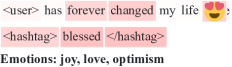
(b)

Figure 1: Attention heat-map visualization. The color intensity corresponds to the weight given to each word by the self-attention mechanism.

In the past, sentiment analysis was tackled by extracting hand-crafted features or features from sentiment lexicons Nielsen (2011); Mohammad and Turney (2010, 2013); Go et al. (2009) that were fed to classifiers such as Naive Bayes or Support Vector Machines (SVM) Bollen et al. (2011a); Mohammad et al. (2013); Kiritchenko et al. (2014). The downside of such approaches is that they require extensive feature engineering from experts and thus they cannot keep up with rapid language evolution Mudinas et al. (2012), especially in social media/micro-blogging context. However, recent advances in artificial neural networks for text classification have shown to outperform conventional approaches Deriu et al. (2016); Rouvier and Favre (2016); Rosenthal et al. (2017a). This can be attributed to their ability to learn features directly from data and also utilize hand-crafted features where needed. Most of aforementioned works focus on sentiment analysis, but similar approaches have been applied to emotion detection  Canales and Martínez-Barco (2014) leading to similar conclusions. SemEval 2018 Task 1: “Affect in Tweets” Mohammad et al. (2018) focuses on exploring emotional content of tweets for both classification and regression tasks concerning the four basic emotions (joy, sadness, anger, fear) and the presence of more fine-grained emotions such as disgust or optimism.

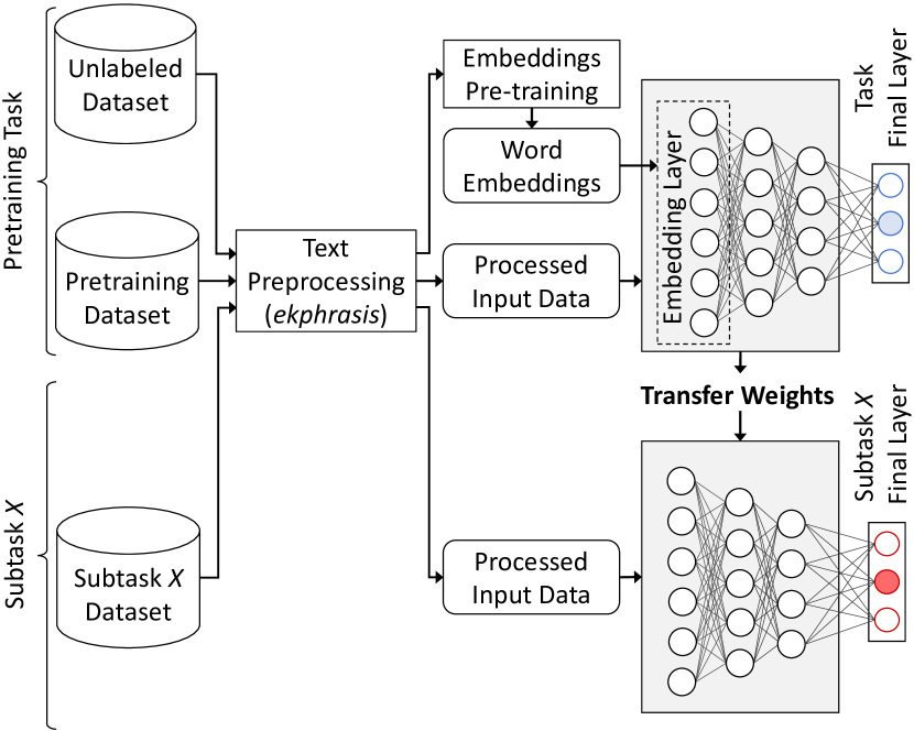
Figure 2: High-level overview of our approach

In this paper, we present a deep-learning system that competed in SemEval 2018 Task 1: “Affect in Tweets”. We explore a transfer learning approach to compensate for limited training data that uses the sentiment analysis dataset of Semeval Task 4A Rosenthal et al. (2017b) for pretraining a model and then further fine-tune it on data for each subtask. Our model operates at the word-level and uses a Bidirectional LSTM equipped with a deep self-attention mechanism Pavlopoulos et al. (2017). Moreover, to help interpret the inner workings of our model, we provide visualizations of tweets with annotations of the salient tokens as predicted by the attention layer.

2 Overview

Figure 2 provides a high-level overview of our approach, which consists of three main steps: (1) the word embeddings pretraining, where we train word2vec and affective word embeddings on our unlabeled Twitter dataset, (2) the transfer learning step, where we pretrain a deep-learning model on a sentiment analysis task, (3) the fine-tuning step, where we fine-tune the pretrained model on each subtask.

Task definitions. Given a tweet we are asked to:

Subtask EI-reg: determine the intensity of a certain emotion (joy, fear, sadness, anger), as a real-valued number between in the $[0,1]$ interval.

Subtask EI-oc: classify its intensity towards a certain emotion (joy, fear, sadness, anger) across a 4-point scale.

Subtask V-oc: classify its valence intensity (i.e sentiment intensity) across a 7-point scale $[-3,3]$.

Subtask V-reg: determine its valence intensity as a real-valued number between in the $[0,1]$ interval.

Subtask E-c: determine the existence of none, one or more out of eleven emotions: anger, anticipation, disgust, fear, joy, love, optimism, pessimism, sadness, surprise, trust.

2.1 Data

Unlabeled Dataset. We collected a big dataset of 550 million English tweets, from April 2014 to June 2017. This dataset is used for (1) calculating word statistics needed in our text preprocessing pipeline (Section 2.3) and (2) training word2vec and affective word embeddings (Section 2.2).

Pretraining Dataset. For transfer learning, we utilized the dataset of Semeval-2017 Task4A. The dataset consists of $61,854$ tweets with $\{positive,neutral,negative\}$ sentiment (valence) annotations. To our knowledge, this is the largest Twitter dataset with affective annotations.

2.2 Word Embeddings

Word embeddings are dense vector representations of words Collobert and Weston (2008); Mikolov et al. (2013), capturing their semantic and syntactic information. To this end, we train word2vec word embeddings, to which we add 10 affective dimensions. We use our pretrained embeddings, to initialize the first layer (embedding layer) of our neural networks.

Word2vec Embeddings. We leverage our unlabeled dataset to train Twitter-specific word embeddings. We use the word2vec  Mikolov et al. (2013) algorithm, with the skip-gram model, negative sampling of 5 and minimum word count of 20, utilizing Gensim’s Řehůřek and Sojka (2010) implementation. The resulting vocabulary contains $800,000$ words.

Affective Embeddings. Starting from small manually annotated lexica, continuous norms (within the $[-1,1]$ interval) for new words are estimated using semantic similarity and a linear model along ten affect-related dimensions, namely: valence, dominance, arousal, pleasantness, anger, sadness, fear, disgust, concreteness, familiarity. The method of generating word level norms is detailed in Malandrakis et al. (2013) and relies on the assumption that given a similarity metric between two words, one may derive the similarity between their affective ratings. This approach uses a set of $N$ words with known affective ratings (seed words), as a starting point. Concretely, we calculate the affective rating of a word $w$ as follows:

$$\hat{\upsilon}(w)=\alpha_{0}+\sum_{i=1}^{N}\alpha_{i}\upsilon(t_{i})S(t_{i},w),$$ (1)

where $t_{1}...t_{N}$ are the seed words, $\upsilon(t_{i})$ is the affective rating for seed word $t_{i}$, $\alpha_{i}$ is a trainable weight corresponding to seed $t_{i}$ and $S(\dot{)}$ stands for the semantic similarity metric between $t_{i}$ and $w$. The seed words $t_{i}$ are selected separately for each dimension, from the words available in the original manual annotations (see 2.2). The $S(\dot{)}$ metric is estimated as shown in Palogiannidi et al. (2015) using word-level contextual feature vectors and adopting a scheme based on mutual information for feature weighting.

Manually annotated norms. To generate affective norms, we need to start from some manual annotations, so we use ten dimensions from four sources. From the Affective Norms for English Words Bradley and Lang (1999) we use norms for valence, arousal and dominance. From the MRC Psycholinguistic database Coltheart (1981), we use norms for concreteness and familiarity. From the Paivio norms Clark and Paivio (2004) we use norms for pleasantness. Finally from Stevenson et al. (2007) we use norms for anger, sadness, fear and disgust.

original	The *new* season of #TwinPeaks is coming on May 21, 2017. CANT WAIT \o/ !!! #tvseries #davidlynch :D
processed	the new <emphasis> season of <hashtag> twin peaks </hashtag> is coming on <date> . cant <allcaps> wait <allcaps> <happy> ! <repeated> <hashtag> tv series </hashtag> <hashtag> david lynch </hashtag> <laugh>

Table 1: Example of our text processor

2.3 Preprocessing

We utilized the ekphrasis Baziotis et al. (2017) tool as a tweet preprocessor. The preprocessing steps included in ekphrasis are: Twitter-specific tokenization, spell correction, word normalization, word segmentation (for splitting hashtags) and word annotation.

Tokenization. Tokenization is the first fundamental preprocessing step and since it is the basis for the other steps, it immediately affects the quality of the features learned by the network. Tokenization on Twitter is challenging, since there is large variation in the vocabulary and the expressions which are used. There are certain expressions which are better kept as one token (e.g. anti-american) and others that should be split into separate tokens. Ekphrasis recognizes Twitter markup, emoticons, emojis, dates (e.g. 07/11/2011, April 23rd), times (e.g. 4:30pm, 11:00 am), currencies (e.g. $10, 25mil, 50€), acronyms, censored words (e.g. s**t), words with emphasis (e.g. *very*) and more using an extensive list of regular expressions.

Normalization. After tokenization, we apply a series of modifications on the extracted tokens, such as spell correction, word normalization and segmentation. Specifically for word normalization we use lowercase words, normalize URLs, emails, numbers, dates, times and user handles (@user). This helps reducing the vocabulary size without losing information. For spell correction Jurafsky and James (2000) and word segmentation Segaran and Hammerbacher (2009) we use the Viterbi algorithm. The prior probabilities are obtained from word statistics from the unlabeled dataset.

The benefits of the aforementioned procedure are the reduction of the vocabulary size, without removing any words, and the preservation of information that is usually lost during tokenization. Table 1 shows an example text snippet and the resulting preprocessed tokens.

2.4 Neural Transfer Learning for NLP

Transfer learning aims to make use of the knowledge from a source domain, to improve the performance of a model in a different, but related, target domain. It has been applied with great success in computer vision (CV) Razavian et al. (2014); Long et al. (2014). Deep neural networks in CV are rarely trained from scratch and instead are initialized with pretrained models. Notable examples include face recognition Taigman et al. (2014) and visual QA  Agrawal et al. (2017), where image features trained on ImageNet  Deng et al. (2009) and word embeddings estimated on large corpora via unsupervised training are combined. Although model transfer has seen widespread success in computer vision, transfer learning beyond pretrained word vectors is less pervasive in NLP.

In our system, we explore the approach of pretraining a network in a sentiment analysis task in Twitter and use it to initialize the weights of the models of each subtask. We chose the dataset of Semeval 2017 Task4A (SA2017) Rosenthal et al. (2017b), which is a semantically similar dataset to the emotion datasets of this task. By pretraining on a dataset in a similar domain, it is more likely that the source and target dataset will have similar distributions.

To build our pretrained model, we initialize the weights of the embedding layer with the word2vec Twitter embeddings and train a bidirectional LSTM (BiLSTM) with a deep self-attention mechanism Pavlopoulos et al. (2017) on SA2017, similar to Baziotis et al. (2017). Afterwards, we utilize the encoding part of the network, which is the BiLSTM and the attention layer, throwing away the last layer. This pretrained model is used for all subtasks, with the addition of a subtask-specific final layer for classification/regression.

2.5 Recurrent Neural Networks

We model the Twitter messages using Recurrent Neural Networks (RNN). RNNs process their inputs sequentially, performing the same operation, $h_{t}=f_{W}(x_{t},h_{t-1})$, on every element in a sequence, where $h_{t}$ is the hidden state $t$ the time step, and $W$ the network weights. We can see that the hidden state at each time step depends on the previous hidden states, thus the order of elements (words) is important. This process also enables RNNs to handle inputs of variable length.

RNNs are difficult to train Pascanu et al. (2013), because gradients may grow or decay exponentially over long sequences Bengio et al. (1994); Hochreiter et al. (2001). A way to overcome these problems is to use more sophisticated variants of regular RNNs, like Long Short-Term Memory (LSTM) networks Hochreiter and Schmidhuber (1997) or Gated Recurrent Units (GRU) Cho et al. (2014), introducing a gating mechanism to ensure proper gradient flow through the network.

2.6 Self-Attention Mechanism

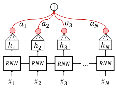
(a) Regular RNN

(b) Attention RNN

Figure 3: Comparison between regular RNN and attentive RNN.

RNNs update their hidden state $h_{i}$ as they process a sequence and the final hidden state holds a summary of the information in the sequence. In order to amplify the contribution of important words in the final representation, a self-attention mechanism Bahdanau et al. (2014) is used as shown in Fig. 3. By employing an attention mechanism, the representation of the input sequence $r$ is no longer limited to just the final state $h_{N}$, but rather it is a combination of all the hidden states $h_{i}$. This is done by computing the sequence representation, as the convex combination of all $h_{i}$. The weights $a_{i}$ are learned by the network and their magnitude signifies the importance of each $h_{i}$ in the final representation. Formally:

$$r=\sum_{i=1}^{N}a_{i}h_{i}\quad where\quad\sum_{i=1}^{N}a_{i}=1,\quad a_{i}>0$$

3 Model Description

Next, we present in detail the submitted models. For all subtasks, we adopted a transfer learning approach, by pretraining a BiLSTM network with a deep attention mechanism on SA2017 dataset. Afterwards, we replaced the last layer of the pretrained model with a task-specific layer and fine-tuned the whole network for each subtask.

3.1 Transfer Learning Model (TF)

Our transfer learning model is based on the sentiment analysis model in Baziotis et al. (2017). It consists of a 2-layer bidirectional LSTM (BiLSTM) with a deep self-attention mechanism.

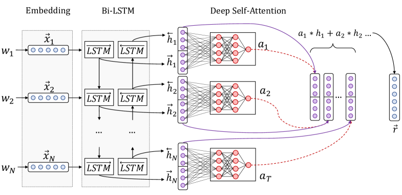
Figure 4: The proposed model, composed of a 2-layer BiLSTM with a deep self-attention mechanism.

Embedding Layer. The input to the network is a Twitter message, treated as a sequence of words. We use an embedding layer to project the words $w_{1},w_{2},...,w_{N}$ to a low-dimensional vector space $R^{W}$, where $W$ is the size of the embedding layer and $N$ the number of words in a tweet. We initialize the weights of the embedding layer with our pre-trained word embeddings (Section 2.2).

BiLSTM Layer. An LSTM takes as input a sequence of word embeddings and produces word annotations $h_{1},h_{2},...,h_{N}$, where $h_{i}$ is the hidden state of the LSTM at time-step $i$, summarizing all the information of the sentence up to $w_{i}$. We use bidirectional LSTMs (BiLSTM) in order to get word annotations that summarize the information from both directions. A BiLSTM consists of $2$ LSTMs, a forward LSTM $\overrightarrow{f}$ that parses the sentence from $w_{1}$ to $w_{N}$ and a backward LSTM $\overleftarrow{f}$ that parses the sentence from $w_{N}$ to $w_{1}$. We obtain the final annotation for each word $h_{i}$, by concatenating the annotations from both directions,

$$h_{i}=\overrightarrow{h_{i}}\parallel\overleftarrow{h_{i}},\quad h_{i}\in R^{2L}$$ (2)

where $\parallel$ denotes the concatenation operation and $L$ the size of each LSTM.

Attention Layer. To amplify the contribution of the most informative words, we augment our BiLSTM with a self-attention mechanism. We use a deep self-attention mechanism Pavlopoulos et al. (2017), to obtain a more accurate estimation of the importance of each word. The attention weight in the simple self-attention mechanism, is replaced with a multilayer perceptron (MLP), composed of $l$ layers with a non-linear activation function ($tanh$). The MLP learns the attention function $g$. The attention weights $a_{i}$ are then computed as a probability distribution over the hidden states $h_{i}$. The final representation $r$ is the convex combination of $h_{i}$ with weights $a_{i}$.

$$e_{i} =g(h_{i})$$ (3)

$$a_{i} =\dfrac{exp(e_{i})}{\sum_{t=1}^{N}exp(e_{t})}$$ (4)

$$r =\sum_{i=1}^{N}a_{i}h_{i},\quad r\in R^{2L}$$ (5)

Output Layer. We use vector $r$ as the feature representation, which we feed to a final task-specific layer. For the regression tasks, we use a fully-connected layer with one neuron and a sigmoid activation function. For the ordinal classification tasks, we use a fully-connected layer, followed by a $softmax$ operation, which outputs a probability distribution over the classes. Finally, for the multilabel classification task, we use a fully-connected layer with 11 neurons (number of labels) and a sigmoid activation function, performing binary classification for each label.

3.2 Fine-Tuning

After training a network on the pretraining dataset (SA2017), we fine-tune it on each subtask, by replacing its final layer with a task-specific layer. We experimented with two fine-tuning schemes. The first approach is to fine-tune the whole network, that is, both the pretrained encoder (BiLSTM) and the task-specific layer. The second approach is to use the pretrained model only for weight initialization, freeze its weights during training and just fine-tune the final layer. Based on the experimental results, the first approach obtains significantly better results in all tasks.

3.3 Regularization

In both models, we add Gaussian noise to the embedding layer, which can be interpreted as a random data augmentation technique, that makes models more robust to overfitting. In addition to that, we use dropout Srivastava et al. (2014) and we stop training after the validation loss has stopped decreasing (early-stopping).

Furthermore, we do not fine-tune the embedding layers. Words occurring in the training set, are projected in the embedding space and the classifier correlates certain regions of the embedding space to certain emotions. However, words included only in the test set, remain at their initial position which may no longer reflect their “true” emotion, leading to mis-classifications.

4 Experiments and Results

4.1 Experimental Setup

Training We use Adam algorithm Kingma and Ba (2014) for optimizing our networks, with mini-batches of size 32 and we clip the norm of the gradients Pascanu et al. (2013) at 1, as an extra safety measure against exploding gradients. For developing our models we used PyTorch Paszke et al. (2017) and Scikit-learn Pedregosa et al. (2011).

Class Weights. In subtasks EI-oc and V-oc, some classes have more training examples than others, introducing bias in our models. To deal with this problem, we apply class weights to the loss function, penalizing more the misclassification of under-represented classes. These weights are computed as the inverse frequencies of the classes in the training set.

Hyper-parameters. In order to tune the hyper-parameter of our model, we adopt a Bayesian optimization Bergstra et al. (2013) approach, performing a more time-efficient search in the high dimensional space of all the possible values, compared to grid or random search. We set size of the embedding layer to 310 (300 word2vec + 10 affective dimensions), which we regularize by adding Gaussian noise with $\sigma=0.2$ and dropout of 0.1. The sentence encoder is composed of 2 BiLSTM layers, each of size 250 (per direction) with a 2-layer self-attention mechanism. Finally, we apply dropout of 0.3 to the encoded representation.

	EI-reg (pearson)				EI-oc (pearson)				V-Reg (pearson)	V-oc (pearson)	E-c (jaccard)
	anger	fear	joy	sadness	anger	fear	joy	sadness
BOW	0.5249	0.5227	0.5716	0.4721	0.3996	0.3491	0.4456	0.3835	0.5963	0.4954	0.4572
NBOW	0.6539	0.6318	0.6355	0.6305	0.5573	0.3796	0.5044	0.5009	0.7501	0.6527	0.4541
NBOW+A*	0.656	0.6359	0.6384	0.6341	0.5367	0.3906	0.4803	0.5005	0.7457	0.6578	0.4478
LSTM-RD	0.7568	0.7357	0.7313	0.7479	0.6387	0.5874	0.6226	0.6343	0.8462	0.7722	0.5788
LSTM-TL-FR	0.7347	0.6509	0.7321	0.7269	0.5999	0.4666	0.6264	0.6030	0.8275	0.7331	0.5243
LSTM-TL-FT	0.7717	0.7273	0.7638	0.7665	0.6329	0.5702	0.6351	0.6400	0.8390	0.7652	0.5788

Table 2: Results of our experiments across all subtasks on the official evaluation metrics. For subtasks EI-reg, EI-oc, V-reg, V-oc, the evaluation metric is Pearson correlation. For subtask E-c, the evaluation metric is multi-label accuracy (Jaccard index). BOW stands for Bag-of-Words baseline, N-BOW stands for Neural Bag-of-Words baseline and N-BOW+A indicates the inclusion of the affective word features. As for the neural models, RD stands for random initialization, TL for Transfer Learning, FR for Frozen pretrained layers (without fine-tuning) and FT for Fine-Tuning. For our deep-learning models, the results are computed by averaging $10$ runs to account for the variability in training performance.

4.2 Experiments

In Table 2, we compare the proposed transfer learning models against 3 strong baselines. Pearson correlation is the metric used for the first four subtasks, whereas Jaccard index is used for the E-c multi-label classification subtask. The first baseline is a unigram Bag-of-Words (BOW) model with TF-IDF weighting. The second baseline is a Neural Bag-of-Words (N-BOW) model, where we retrieve the word2vec embeddings of the words in a tweet and compute the tweet representation as the average (centroid) of the constituent word2vec embeddings. Finally, the third baseline is similar to the second one, but with the addition of 10-dimensional affective embeddings that model affect-related dimensions (valence, dominance, arousal, etc). Both BOW and N-BOW features are then fed to a linear SVM classifier, with tuned $C=0.6$. In order to assess the impact of transfer learning, we evaluate the performance of each model in 3 different settings: (1) random weight initialization (LSTM-RD), (2) transfer learning with frozen weights (LSTM-TL-FR), (3) transfer learning with finetuning (LSTM-TL-FT). The results of our neural models in Table 2 are computed by averaging the results of $10$ runs to account for model variability.

Baselines. Our first observation is that N-BOW baselines significantly outperform BOW in subtasks EI-reg, EI-oc, V-reg and V-oc, in which we have to predict the intensity of an emotion, or the tweet’s valence. However, BOW achieves slightly better performance in subtask E-c, in which we have to recognize the emotions expressed in each tweet. This can be attributed to the fact that BOW models perform well in tasks where we the occurrence of certain words is sufficient, to accurately determine the classification result. This suggests that in subtask E-c, certain words are highly indicative of some emotions. Word embeddings, though, that encode the correlation of each word with different dimensions, enable NBOW to better predict the intensity of various emotions. Furthermore, regarding the affective embeddings, we can directly observe their impact by the performance gain over the NBOW baseline.

Transfer Learning. We observe that our neural models achieved better performance than all baselines by a large margin. Moreover, we can see that our transfer learning model yielded higher performance over the non-transfer model in most of the Emotion Intensity (EI) subtasks. In the Emotion multi-label classification subtask (E-c), transfer learning did not outperform the random initialization model. This can be attributed to the fact that our source dataset (SA17) was not diverse enough to boost the model performance when classifying the tweets into none, one or more of a set of 11 emotions. As for fine-tuning or freezing the pretrained layers, the overall results show that enabling the model to fine-tune always results in significant gains. This is consistent with our intuition that allowing the weights of the model to adapt to the target dataset, thus encoding task-specific information, results in performance gains. Regarding the emotion of joy, we observe that in EI-reg and EI-oc subtasks, LSTM-RD matches the performance of LSTM-TL-FR. We interpret this result as an indication of the semantic similarity between the source and the target task.

	Ave.diff. Overall	Ave.diff.	p-value
Anger	0.001	0	0.02223
Fear	-0.003	-0.003	0
Joy	0.004	0.010	0
Sadness	0.002	-0.002	0
Valence	0.005	0.005	0

Table 3: Analysis for inappropriate biases

Mystery dataset. The submitted models were also evaluated against a mystery dataset, in order to investigate if there is statistically significant social bias in them. This is a very important experiment, especially when automated machine learning algorithms are interacting with social media content and users in the wild. The mystery dataset consists of pairs of sentences that differ only in the social context (e.g. gender or race). Submitted models are expected to predict the same affective values for both sentences in the pair. The evaluation metric is the average difference in prediction scores per class, along with the p-value score indicating if the difference is statistically significant. Results are summarized in Table 3.

4.3 Attention visualizations

Fig. 10 shows a heat-map of the attention weights on top of 8 example tweets (2 tweets per emotion). The color intensity corresponds to the weight given to each word by the self-attention mechanism and signifies the importance of this word for the final prediction. We can see that the salient words correspond to the predicted emotion (e.g. “irritated” for anger, “mourn” for sadness etc.). An interesting observation is that when emojis are present they are almost always selected as important, which indicates their function as weak annotations. Also note that the attention mechanism can hint to dependencies between words even if they far in a sentence, like the “why” and “mad” in the sadness example.

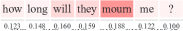
Figure 5: Examples of intensity of joy

Figure 6: Examples of intensity of sadness

Figure 7: Examples of intensity of fear

Figure 8: Examples of intensity of anger

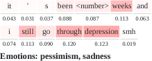
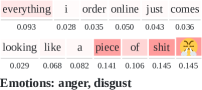
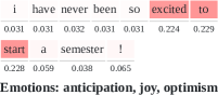
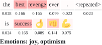
Figure 9: Examples of emotion recognition

Figure 10: Attention heat-map visualization. The color intensity of each word corresponds to its weight (importance), given by the self-attention mechanism (Section 2.6).

4.4 Competition Results

Our official ranking was 2/48 in subtask 1A (EI-reg), 5/39 in subtask 2A (EI-oc), 4/38 in subtask 3A (V-reg), 8/37 (tie with 6 and 7 place) in subtask 4A (V-oc) and 1/35 in subtask 5A (E-c). All of our models achieved competitive results. We used the same transfer learning approach in all subtasks (LSTM-TL-FT), utilizing the same pretrained model.

5 Conclusion

In this paper we present a deep-learning system for short text emotion intensity, valence estimation for both regression and classification and multi-class emotion classification. We used Bidirectional LSTMs, with a deep attention mechanism and took advantage of transfer learning in order to address the problem of limited training data.

Our models achieved excellent results in single and multi-label classification tasks, but mixed results in emotion and valence intensity tasks. Future work can follow two directions. Firstly, we aim to revisit the task with different transfer learning approaches, such as Felbo et al. (2017); Howard and Ruder (2018); Hashimoto et al. (2016). Secondly, we would like to introduce character-level information in our models, based on Wieting et al. (2016); Labeau and Allauzen (2017), in order to overcome the problem of out-of-vocabulary (OOV) words and learn syntactic and stylistic features Peters et al. (2018), which are highly indicative of emotions and their intensity.

Finally, we make both our pretrained word embeddings and the source code of our models available to the community, in order to make our results easily reproducible and facilitate further experimentation in the field.

Acknowledgements. This work has been partially supported by the BabyRobot project supported by EU H2020 (grant #687831). Also, the authors would like to thank NVIDIA for supporting this work by donating a TitanX GPU.

References

- Agrawal et al. (2017) Aishwarya Agrawal, Jiasen Lu, Stanislaw Antol, Margaret Mitchell, C. Lawrence Zitnick, Devi Parikh, and Dhruv Batra. 2017. Vqa: Visual question answering. Int. J. Comput. Vision, 123(1):4–31.
- Bahdanau et al. (2014) Dzmitry Bahdanau, Kyunghyun Cho, and Yoshua Bengio. 2014. Neural machine translation by jointly learning to align and translate. CoRR, abs/1409.0473.
- Baziotis et al. (2017) Christos Baziotis, Nikos Pelekis, and Christos Doulkeridis. 2017. Datastories at semeval-2017 task 4: Deep lstm with attention for message-level and topic-based sentiment analysis. In Proceedings of the 11th International Workshop on Semantic Evaluation (SemEval-2017), pages 747–754.
- Bengio et al. (1994) Yoshua Bengio, Patrice Simard, and Paolo Frasconi. 1994. Learning long-term dependencies with gradient descent is difficult. IEEE transactions on neural networks, 5(2):157–166.
- Bergstra et al. (2013) James Bergstra, Daniel Yamins, and David D. Cox. 2013. Making a Science of Model Search: Hyperparameter Optimization in Hundreds of Dimensions for Vision Architectures. ICML (1), 28:115–123.
- Bollen et al. (2011a) Johan Bollen, Huina Mao, and Alberto Pepe. 2011a. Modeling public mood and emotion: Twitter sentiment and socio-economic phenomena. Icwsm, 11:450–453.
- Bollen et al. (2011b) Johan Bollen, Huina Mao, and Xiaojun Zeng. 2011b. Twitter mood predicts the stock market. Journal of computational science, 2(1):1–8.
- Bradley and Lang (1999) M. Bradley and P. Lang. 1999. Affective norms for English words (ANEW): Instruction Manual and Affective Ratings. Technical report.
- Canales and Martínez-Barco (2014) Lea Canales and Patricio Martínez-Barco. 2014. Emotion detection from text: A survey. In Proceedings of the Workshop on Natural Language Processing in the 5th Information Systems Research Working Days (JISIC), pages 37–43.
- Chamlertwat et al. (2012) Wilas Chamlertwat, Pattarasinee Bhattarakosol, Tippakorn Rungkasiri, and Choochart Haruechaiyasak. 2012. Discovering consumer insight from twitter via sentiment analysis. J. UCS, 18(8):973–992.
- Cho et al. (2014) Kyunghyun Cho, Bart Van Merriënboer, Caglar Gulcehre, Dzmitry Bahdanau, Fethi Bougares, Holger Schwenk, and Yoshua Bengio. 2014. Learning phrase representations using RNN encoder-decoder for statistical machine translation. arXiv preprint arXiv:1406.1078.
- Clark and Paivio (2004) J.M. Clark and A. Paivio. 2004. Extensions of the paivio, yuille, and madigan (1968) norms. Behavior Research Methods, Instruments, & Computers, 36(3):371–383.
- Collobert and Weston (2008) Ronan Collobert and Jason Weston. 2008. A unified architecture for natural language processing: Deep neural networks with multitask learning. In Proceedings of the 25th International Conference on Machine Learning, pages 160–167. ACM.
- Coltheart (1981) M. Coltheart. 1981. The mrc psycholinguistic database. The Quarterly Journal of Experimental Psychology Section A, 33(4):497–505.
- Deng et al. (2009) Jia Deng, Wei Dong, Richard Socher, Li-Jia Li, Kai Li, and Fei-Fei Li. 2009. Imagenet: a large-scale hierarchical image database.
- Deriu et al. (2016) Jan Deriu, Maurice Gonzenbach, Fatih Uzdilli, Aurelien Lucchi, Valeria De Luca, and Martin Jaggi. 2016. SwissCheese at SemEval-2016 Task 4: Sentiment classification using an ensemble of convolutional neural networks with distant supervision. Proceedings of SemEval, pages 1124–1128.
- Felbo et al. (2017) Bjarke Felbo, Alan Mislove, Anders Søgaard, Iyad Rahwan, and Sune Lehmann. 2017. Using millions of emoji occurrences to learn any-domain representations for detecting sentiment, emotion and sarcasm. arXiv preprint arXiv:1708.00524.
- Go et al. (2009) Alec Go, Richa Bhayani, and Lei Huang. 2009. Twitter sentiment classification using distant supervision. CS224N Project Report, Stanford, 1(12).
- Hashimoto et al. (2016) Kazuma Hashimoto, Caiming Xiong, Yoshimasa Tsuruoka, and Richard Socher. 2016. A joint many-task model: Growing a neural network for multiple nlp tasks. arXiv preprint arXiv:1611.01587.
- Hochreiter et al. (2001) Sepp Hochreiter, Yoshua Bengio, Paolo Frasconi, and Jürgen Schmidhuber. 2001. Gradient Flow in Recurrent Nets: The Difficulty of Learning Long-Term Dependencies. A field guide to dynamical recurrent neural networks. IEEE Press.
- Hochreiter and Schmidhuber (1997) Sepp Hochreiter and Jürgen Schmidhuber. 1997. Long short-term memory. Neural computation, 9(8):1735–1780.
- Howard and Ruder (2018) Jeremy Howard and Sebastian Ruder. 2018. Fine-tuned language models for text classification. arXiv preprint arXiv:1801.06146.
- Jurafsky and James (2000) Daniel Jurafsky and H. James. 2000. Speech and language processing an introduction to natural language processing, computational linguistics, and speech.
- Kingma and Ba (2014) Diederik Kingma and Jimmy Ba. 2014. Adam: A method for stochastic optimization. arXiv preprint arXiv:1412.6980.
- Kiritchenko et al. (2014) Svetlana Kiritchenko, Xiaodan Zhu, and Saif M. Mohammad. 2014. Sentiment analysis of short informal texts. Journal of Artificial Intelligence Research, 50:723–762.
- Labeau and Allauzen (2017) Matthieu Labeau and Alexandre Allauzen. 2017. Character and subword-based word representation for neural language modeling prediction. In Proceedings of the First Workshop on Subword and Character Level Models in NLP, pages 1–13.
- Long et al. (2014) Jonathan Long, Evan Shelhamer, and Trevor Darrell. 2014. Fully convolutional networks for semantic segmentation. CoRR, abs/1411.4038.
- Malandrakis et al. (2013) N. Malandrakis, A. Potamianos, E. Iosif, and S. Narayanan. 2013. Distributional semantic models for affective text analysis. IEEE Transactions on Audio, Speech and Language Processing, 21(11):2379–2392.
- Mikolov et al. (2013) Tomas Mikolov, Ilya Sutskever, Kai Chen, Greg S. Corrado, and Jeff Dean. 2013. Distributed representations of words and phrases and their compositionality. In Advances in Neural Information Processing Systems, pages 3111–3119.
- Mohammad et al. (2018) Saif M. Mohammad, Felipe Bravo-Marquez, Mohammad Salameh, and Svetlana Kiritchenko. 2018. Semeval-2018 Task 1: Affect in tweets. In Proceedings of International Workshop on Semantic Evaluation (SemEval-2018), New Orleans, LA, USA.
- Mohammad et al. (2013) Saif M. Mohammad, Svetlana Kiritchenko, and Xiaodan Zhu. 2013. NRC-Canada: Building the state-of-the-art in sentiment analysis of tweets. arXiv preprint arXiv:1308.6242.
- Mohammad and Turney (2010) Saif M Mohammad and Peter D Turney. 2010. Emotions evoked by common words and phrases: Using mechanical turk to create an emotion lexicon. In Proceedings of the NAACL HLT 2010 workshop on computational approaches to analysis and generation of emotion in text, pages 26–34. Association for Computational Linguistics.
- Mohammad and Turney (2013) Saif M Mohammad and Peter D Turney. 2013. Crowdsourcing a word–emotion association lexicon. Computational Intelligence, 29(3):436–465.
- Mudinas et al. (2012) Andrius Mudinas, Dell Zhang, and Mark Levene. 2012. Combining lexicon and learning based approaches for concept-level sentiment analysis. In Proceedings of the first international workshop on issues of sentiment discovery and opinion mining, page 5. ACM.
- Nielsen (2011) Finn Årup Nielsen. 2011. A new anew: Evaluation of a word list for sentiment analysis in microblogs. arXiv preprint arXiv:1103.2903.
- Palogiannidi et al. (2015) E. Palogiannidi, E. Iosif, P. Koutsakis, and A. Potamianos. 2015. Valence, Arousal and Dominance Estimation for English, German, Greek, Portuguese and Spanish Lexica using Semantic Models. In Proc. of Interspeech, pages 1527–1531.
- Pascanu et al. (2013) Razvan Pascanu, Tomas Mikolov, and Yoshua Bengio. 2013. On the difficulty of training recurrent neural networks. ICML (3), 28:1310–1318.
- Paszke et al. (2017) Adam Paszke, Sam Gross, Soumith Chintala, Gregory Chanan, Edward Yang, Zachary DeVito, Zeming Lin, Alban Desmaison, Luca Antiga, and Adam Lerer. 2017. Automatic differentiation in pytorch.
- Pavlopoulos et al. (2017) John Pavlopoulos, Prodromos Malakasiotis, and Ion Androutsopoulos. 2017. Deep learning for user comment moderation. arXiv preprint arXiv:1705.09993.
- Pedregosa et al. (2011) Fabian Pedregosa, Gaël Varoquaux, Alexandre Gramfort, Vincent Michel, Bertrand Thirion, Olivier Grisel, Mathieu Blondel, Peter Prettenhofer, Ron Weiss, Vincent Dubourg, and others. 2011. Scikit-learn: Machine learning in Python. Journal of Machine Learning Research, 12(Oct):2825–2830.
- Peters et al. (2018) Matthew E Peters, Mark Neumann, Mohit Iyyer, Matt Gardner, Christopher Clark, Kenton Lee, and Luke Zettlemoyer. 2018. Deep contextualized word representations. arXiv preprint arXiv:1802.05365.
- Pla and Hurtado (2014) Ferran Pla and Lluís-F Hurtado. 2014. Political tendency identification in twitter using sentiment analysis techniques. In Proceedings of COLING 2014, the 25th international conference on computational linguistics: Technical Papers, pages 183–192.
- Razavian et al. (2014) Ali Sharif Razavian, Hossein Azizpour, Josephine Sullivan, and Stefan Carlsson. 2014. CNN features off-the-shelf: an astounding baseline for recognition. CoRR, abs/1403.6382.
- Řehůřek and Sojka (2010) Radim Řehůřek and Petr Sojka. 2010. Software Framework for Topic Modelling with Large Corpora. In Proceedings of the LREC 2010 Workshop on New Challenges for NLP Frameworks, pages 45–50, Valletta, Malta. ELRA. http://is.muni.cz/publication/884893/en.
- Rosenthal et al. (2017a) Sara Rosenthal, Noura Farra, and Preslav Nakov. 2017a. Semeval-2017 task 4: Sentiment analysis in twitter. In Proceedings of the 11th International Workshop on Semantic Evaluation (SemEval-2017), pages 502–518.
- Rosenthal et al. (2017b) Sara Rosenthal, Noura Farra, and Preslav Nakov. 2017b. SemEval-2017 Task 4: Sentiment Analysis in Twitter. In Proceedings of the 11th International Workshop on Semantic Evaluation, SemEval ’17, Vancouver, Canada. Association for Computational Linguistics.
- Rouvier and Favre (2016) Mickael Rouvier and Benoit Favre. 2016. SENSEI-LIF at SemEval-2016 Task 4: Polarity embedding fusion for robust sentiment analysis. Proceedings of SemEval, pages 202–208.
- Segaran and Hammerbacher (2009) Toby Segaran and Jeff Hammerbacher. 2009. Beautiful Data: The Stories Behind Elegant Data Solutions. "O’Reilly Media, Inc.".
- Si et al. (2013) Jianfeng Si, Arjun Mukherjee, Bing Liu, Qing Li, Huayi Li, and Xiaotie Deng. 2013. Exploiting topic based twitter sentiment for stock prediction. In Proceedings of the 51st Annual Meeting of the Association for Computational Linguistics (Volume 2: Short Papers), volume 2, pages 24–29.
- Srivastava et al. (2014) Nitish Srivastava, Geoffrey E. Hinton, Alex Krizhevsky, Ilya Sutskever, and Ruslan Salakhutdinov. 2014. Dropout: A simple way to prevent neural networks from overfitting. Journal of Machine Learning Research, 15(1):1929–1958.
- Stevenson et al. (2007) R.A. Stevenson, J.A. Mikels, and T.W. James. 2007. Characterization of the affective norms for english words by discrete emotional categories. Behavior research methods, 39(4):1020–1024.
- Taigman et al. (2014) Yaniv Taigman, Ming Yang, Marc’Aurelio Ranzato, and Lior Wolf. 2014. Deepface: Closing the gap to human-level performance in face verification.
- Tumasjan et al. (2010) Andranik Tumasjan, Timm Oliver Sprenger, Philipp G Sandner, and Isabell M Welpe. 2010. Predicting elections with twitter: What 140 characters reveal about political sentiment. Icwsm, 10(1):178–185.
- Wieting et al. (2016) John Wieting, Mohit Bansal, Kevin Gimpel, and Karen Livescu. 2016. Charagram: Embedding words and sentences via character n-grams. arXiv preprint arXiv:1607.02789.