NTUA-SLP at SemEval-2018 Task 2: Predicting Emojis using RNNs with Context-aware Attention

Abstract

In this paper we present a deep-learning model that competed at SemEval-2018 Task 2 “Multilingual Emoji Prediction”. We participated in subtask A, in which we are called to predict the most likely associated emoji in English tweets. The proposed architecture relies on a Long Short-Term Memory network, augmented with an attention mechanism, that conditions the weight of each word, on a “context vector” which is taken as the aggregation of a tweet’s meaning. Moreover, we initialize the embedding layer of our model, with word2vec word embeddings, pretrained on a dataset of 550 million English tweets. Finally, our model does not rely on hand-crafted features or lexicons and is trained end-to-end with back-propagation. We ranked 2 out of 48 teams.

1 Introduction

Emojis play an important role in textual communication, as they function as a substitute for non-verbal cues, that are taken for granted in face-to-face communication, thus allowing users to convey emotions by means other than words. Despite their large appeal in text, they haven’t received much attention until recently. Former works, mostly consider their semantics Aoki and Uchida (2011); Espinosa-Anke et al. (2016); Barbieri et al. (2016b, a); Ljubešić and Fišer (2016); Eisner et al. (2016) and only recently their role in social media was explored Barbieri et al. (2017); Cappallo et al. (2018). In SemEval-2018 Task 2: “Multilingual Emoji Prediction” Barbieri et al. (2018), given a tweet, we are asked to predict its most likely associated emoji.

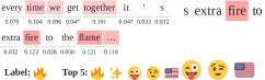
Figure 1: Attention heat-map visualization. The color intensity corresponds to the weight given to each word by the self-attention mechanism.

In this work, we present a near state of the art approach for predicting emojis in tweets, which outperforms the best present work Barbieri et al. (2017). For this purpose, we employ an LSTM network augmented with a context-aware self-attention mechanism, producing a feature representation used for classification. Moreover, the attention mechanism helps us make our model’s behavior more interpretable, by examining the distribution of the attention weights for a given tweet. To this end, we provide visualizations with the distributions of the attention weights.

2 Overview

Figure 3 provides a high-level overview of our approach that consists of three main steps: (1) The text preprocessing step, which is common both for unlabeled data and the task’s dataset, (2) the word embeddings pre-training step, where we train custom word embeddings on a big collection of unlabeled Twitter messages and (3) the model training step where we train the deep learning model.

Task definition. In subtask A, given an English tweet, we are called to predict the most likely associated emoji, from the 20 most frequent emojis in English tweets according to Barbieri et al. (2017). The training dataset consists of 500k tweets, retrieved from October 2015 to February 2017 and geolocalized in the United States. Fig. 2 shows the classes (emojis) and their distribution.

$\begin{array}[]{ccccc}\includegraphics[height=10.52737pt,width=10.52737pt]{images/red_heart.png}&\includegraphics[height=10.52737pt,width=10.52737pt]{images/smiling_face_with_hearteyes.png}&\includegraphics[height=10.52737pt,width=10.52737pt]{images/face_with_tears_of_joy.png}&\includegraphics[height=10.52737pt,width=10.52737pt]{images/two_hearts.png}&\includegraphics[height=10.52737pt,width=10.52737pt]{images/fire.png}\\ 22.42\%&10.34\%&10.18\%&5.48\%&4.91\%\vspace{-4pt}\\ \\ \includegraphics[height=10.52737pt,width=10.52737pt]{images/smiling_face_with_smiling_eyes.png}&\includegraphics[height=10.52737pt,width=10.52737pt]{images/smiling_face_with_sunglasses.png}&\includegraphics[height=10.52737pt,width=10.52737pt]{images/sparkles.png}&\includegraphics[height=10.52737pt,width=10.52737pt]{images/blue_heart.png}&\includegraphics[height=10.52737pt,width=10.52737pt]{images/face_blowing_a_kiss.png}\\ 4.67\%&4.26\%&3.64\%&3.40\%&3.23\%\vspace{-4pt}\\ \\ \includegraphics[height=10.52737pt,width=10.52737pt]{images/camera.png}&\includegraphics[height=10.52737pt,width=10.52737pt]{images/United_States.png}&\includegraphics[height=10.52737pt,width=10.52737pt]{images/sun.png}&\includegraphics[height=10.52737pt,width=10.52737pt]{images/purple_heart.png}&\includegraphics[height=10.52737pt,width=10.52737pt]{images/winking_face.png}\\ 3.22\%&3.04\%&2.90\%&2.60\%&2.70\%\vspace{-4pt}\\ \\ \includegraphics[height=10.52737pt,width=10.52737pt]{images/hundred_points.png}&\includegraphics[height=10.52737pt,width=10.52737pt]{images/beaming_face_with_smiling_eyes.png}&\includegraphics[height=10.52737pt,width=10.52737pt]{images/Christmas_tree.png}&\includegraphics[height=10.52737pt,width=10.52737pt]{images/camera_with_flash.png}&\includegraphics[height=10.52737pt,width=10.52737pt]{images/winking_face_with_tongue.png}\\ 2.68\%&2.61\%&2.58\%&2.66\%&2.48\%\end{array}$

Figure 2: Distribution of emoji (class) labels.

2.1 Data

Unlabeled Dataset. We collected a dataset of 550 million archived English Twitter messages, from Apr. 2014 to Jun. 2017. This dataset is used for (1) calculating word statistics needed in our text preprocessing pipeline (Section 2.2) and (2) training word2vec word embeddings.

Word Embeddings. We leverage our unlabeled dataset to train Twitter-specific word embeddings. We use the word2vec  Mikolov et al. (2013) algorithm, with the skip-gram model, negative sampling of 5 and minimum word count of 20, utilizing the Gensim’s Řehůřek and Sojka (2010) implementation. The resulting vocabulary contains $800,000$ words. The pre-trained word embeddings are used for initializing the first layer (embedding layer) of our neural networks.

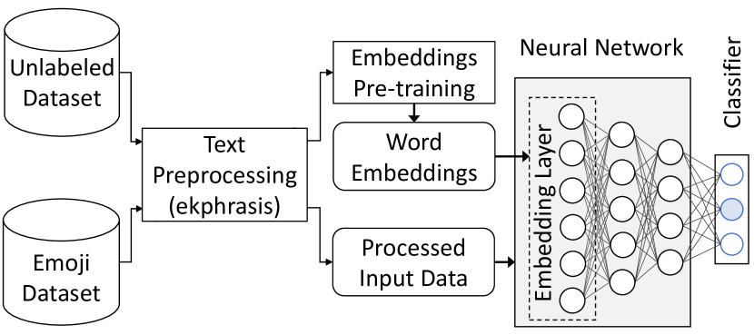
Figure 3: High-level overview of our approach

original	The *new* season of #TwinPeaks is coming on May 21, 2017. CANT WAIT \o/ !!! #tvseries #davidlynch :D
processed	the new <emphasis> season of <hashtag> twin peaks </hashtag> is coming on <date> . cant <allcaps> wait <allcaps> <happy> ! <repeated> <hashtag> tv series </hashtag> <hashtag> david lynch </hashtag> <laugh>

Table 1: Example of our text processor

2.2 Preprocessing

We utilized the ekphrasis tool Baziotis et al. (2017) as a tweet preprocessor. The preprocessing steps included in ekphrasis are: Twitter-specific tokenization, spell correction, word normalization, word segmentation (for splitting hashtags) and word annotation.

Tokenization. Tokenization is the first fundamental preprocessing step and since it is the basis for the other steps, it immediately affects the quality of the features learned by the network. Tokenization on Twitter is challenging, since there is large variation in the vocabulary and the expressions which are used. There are certain expressions which are better kept as one token (e.g. anti-american) and others that should be split into separate tokens. Ekphraris recognizes Twitter markup, emoticons, emojis, dates (e.g. 07/11/2011, April 23rd), times (e.g. 4:30pm, 11:00 am), currencies (e.g. $10, 25mil, 50€), acronyms, censored words (e.g. s**t), words with emphasis (e.g. *very*) and more using an extensive list of regular expressions.

Normalization. After tokenization we apply a series of modifications on extracted tokens, such as spell correction, word normalization and segmentation. Specifically for word normalization we lowercase words, normalize URLs, emails, numbers, dates, times and user handles (@user). This helps reducing the vocabulary size without losing information. For spell correction Jurafsky and James (2000) and word segmentation Segaran and Hammerbacher (2009) we use the Viterbi algorithm. The prior probabilities are initialized using uni/bi-gram word statistics from the unlabeled dataset. Table 1 shows an example text snippet and the resulting preprocessed tokens.

2.3 Recurrent Neural Networks

We model the Twitter messages using Recurrent Neural Networks (RNN). RNNs process their inputs sequentially, performing the same operation, $h_{t}=f_{W}(x_{t},h_{t-1})$, on every element in a sequence, where $h_{t}$ is the hidden state $t$ the time step, and $W$ the network weights. We can see that hidden state at each time step depends on previous hidden states, thus the order of elements (words) is important. This process also enables RNNs to handle inputs of variable length.

RNNs are difficult to train Pascanu et al. (2013), because gradients may grow or decay exponentially over long sequences Bengio et al. (1994); Hochreiter et al. (2001). A way to overcome these problems is to use more sophisticated variants of regular RNNs, like Long Short-Term Memory (LSTM) networks Hochreiter and Schmidhuber (1997) or Gated Recurrent Units (GRU) Cho et al. (2014), which ensure better gradient flow through the network.

(a) Regular RNN

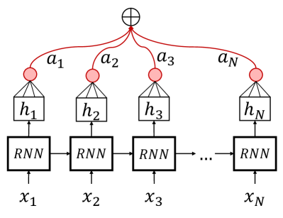
(b) Attention RNN

Figure 4: Comparison between the regular RNN and the RNN with attention.

Self-Attention Mechanism. RNNs update their hidden state $h_{i}$ as they process a sequence and the final hidden state holds a summary of the information in the sequence. In order to amplify the contribution of important words in the final representation, a self-attention mechanism Bahdanau et al. (2014) can be used (Fig. 4). In normal RNNs, we use as representation $r$ of the input sequence its final state $h_{N}$. However, using an attention mechanism, we compute $r$ as the convex combination of all $h_{i}$, with weights $a_{i}$, which signify the importance of each hidden state. Formally: $r=\sum_{i=1}^{N}a_{i}h_{i},\mbox{where}\sum_{i=1}^{N}a_{i}=1,\;\mbox{and}\;a_{i}>0.$

3 Model Description

We use a word-level BiLSTM architecture to model semantic information in tweets. We also propose an attention mechanism, which conditions the weight of $h_{i}$ on a “context vector” that is taken as the aggregation of the tweet meaning.

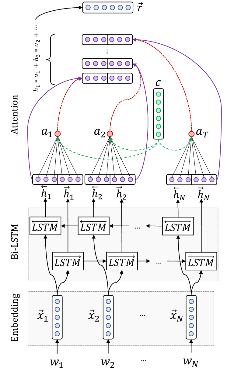
Figure 5: Architecture of the proposed model.

Embedding Layer. The input to the network is a Twitter message, treated as a sequence of words. We use an embedding layer to project the words $w_{1},w_{2},...,w_{N}$ to a low-dimensional vector space $R^{W}$, where $W$ the size of the embedding layer and $N$ the number of words in a tweet. We initialize the weights of the embedding layer with our pretrained word embeddings.

BiLSTM Layer. A LSTM takes as input the words of a tweet and produces the word annotations $h_{1},h_{2},...,h_{N}$, where $h_{i}$ is the hidden state of the LSTM at time-step $i$, summarizing all the information of the sentence up to $w_{i}$. We use bidirectional LSTM (BiLSTM) in order to get word annotations that summarize the information from both directions. A BiLSTM consists of a forward LSTM $\overrightarrow{f}$ that reads the sentence from $w_{1}$ to $w_{N}$ and a backward LSTM $\overleftarrow{f}$ that reads the sentence from $w_{N}$ to $w_{1}$. We obtain the final annotation for each word, by concatenating the annotations from both directions, $h_{i}=\overrightarrow{h_{i}}\parallel\overleftarrow{h_{i}},\quad h_{i}\in R^{2L}$ where $\parallel$ denotes the concatenation operation and $L$ the size of each LSTM.

Context-aware Self-Attention Layer. Even though the hidden state $h_{i}$ of the LSTM captures the local context up to word $i$, in order to better estimate the importance of each word given the context of the tweet we condition hidden state on a context vector. The context vector is taken as the average of $h_{i}$: $c=\dfrac{1}{N}\sum_{1}^{N}h_{i}$. The context-aware annotations $u_{i}$ are obtained as the concatenation of $c$ and $h_{i}$: $u_{i}=h_{i}\parallel c$. The attention weights $a_{i}$ are computed as the softmax of the attention layer outputs $e_{i}$. $W$ and $b$ are the trainable weights and biases of the attention layer:

$$e_{i} =tanh(Wu_{i}+b)$$ (1)

$$a_{i} =\dfrac{exp(e_{i})}{\sum_{t=1}^{N}exp(e_{t})}$$ (2)

The final representation $r$ is again taken as the convex combination of the hidden states.

$$r=\sum_{i=1}^{N}a_{i}h_{i},\quad r\in R^{2L}$$ (3)

Output Layer. We use the representation $r$ as feature vector for classification and we feed it to a fully-connected softmax layer with $L$ neurons, which outputs a probability distribution over all classes $p_{c}$ as described in Eq. 4:

$$p_{c}=\frac{e^{Wr+b}}{\sum_{i\in[1,L]}(e^{W_{i}r+b_{i}})}$$ (4)

where $W$ and $b$ are the layer’s weights and biases.

3.1 Regularization

In both models we add Gaussian noise to the embedding layer, which can be interpreted as a random data augmentation technique, that makes models more robust to overfitting. In addition to that we use dropout Srivastava et al. (2014) and we stop training after the validation loss has stopped decreasing (early-stopping).

4 Experiments and Results

4.1 Experimental Setup

Class Weights. In order to deal with class imbalances, we apply class weights to the loss function of our models, penalizing more the misclassification of underrepresented classes. We weight each class by its inverse frequency in the training set.

Training We use Adam algorithm Kingma and Ba (2014) for optimizing our networks, with mini-batches of size 32 and we clip the norm of the gradients Pascanu et al. (2013) at 1, as an extra safety measure against exploding gradients. For developing our models we used PyTorch Paszke et al. (2017) and Scikit-learn Pedregosa et al. (2011).

Hyper-parameters. In order to find good hyper-parameter values in a relative short time (compared to grid or random search), we adopt the Bayesian optimization Bergstra et al. (2013) approach, performing a time-efficient search in the space of all hyper-parameter values. The size of the embedding layer is 300, and the LSTM layers 300 (600 for BiLSTM). We add Gaussian noise with $\sigma=0.05$ and dropout of 0.1 at the embedding layer and dropout of 0.3 at the LSTM layer.

Results. The dataset for Task 2 was introduced in Saggion et al. (2017), where the authors propose a character level model with pretrained word vectors that achieves an F1 score of $34\%$. Our ranking as shown in Table 2 was 2/49, with an F1 score of $35.361\%$, which was the official evaluation metric, while team TueOslo achieved the first position with an F1 score of $35.991\%$. It should be noted that only the first $2$ teams managed to surpass the baseline model presented in Saggion et al. (2017).

#	Team Name	Acc	Prec	Rec	F1
1	TueOslo	47.094	36.551	36.222	35.991
2	NTUA-SLP	44.744	34.534	37.996	35.361
3	Unknown	45.548	34.997	33.572	34.018
4	Liu Man	47.464	39.426	33.695	33.665

Table 2: Official Results for Subtask A

	f1	accuracy	recall	precision
BOW	0.3370	0.4468	0.3321	0.3525
N-BOW	0.2904	0.4120	0.2849	0.3150
CA-LSTM	0.3564	0.4482	0.3885	0.3531

Table 3: Comparison against baselines

In Table 3 we compare the proposed Context-Attention LSTM (CA-LSTM) model against 2 baselines: (1) a Bag-of-Words (BOW) model with TF-IDF weighting and (2) a Neural Bag-of-Words (N-BOW) model, where we retrieve the word2vec representations of the words in a tweet and compute the tweet representation as the centroid of the constituent word2vec representations. Both BOW and N-BOW features are then fed to a linear SVM classifier, with tuned $C=0.6$. The CA-LSTM results in Table 3 are computed by averaging the results of $10$ runs to account for model variability. Table 3 shows that BOW model outperforms N-BOW by a large margin, which may indicate that there exist words, which are very correlated with specific classes and their occurrence can determine the classification result. Finally, we observe that CA-LSTM significantly outperforms both baselines.

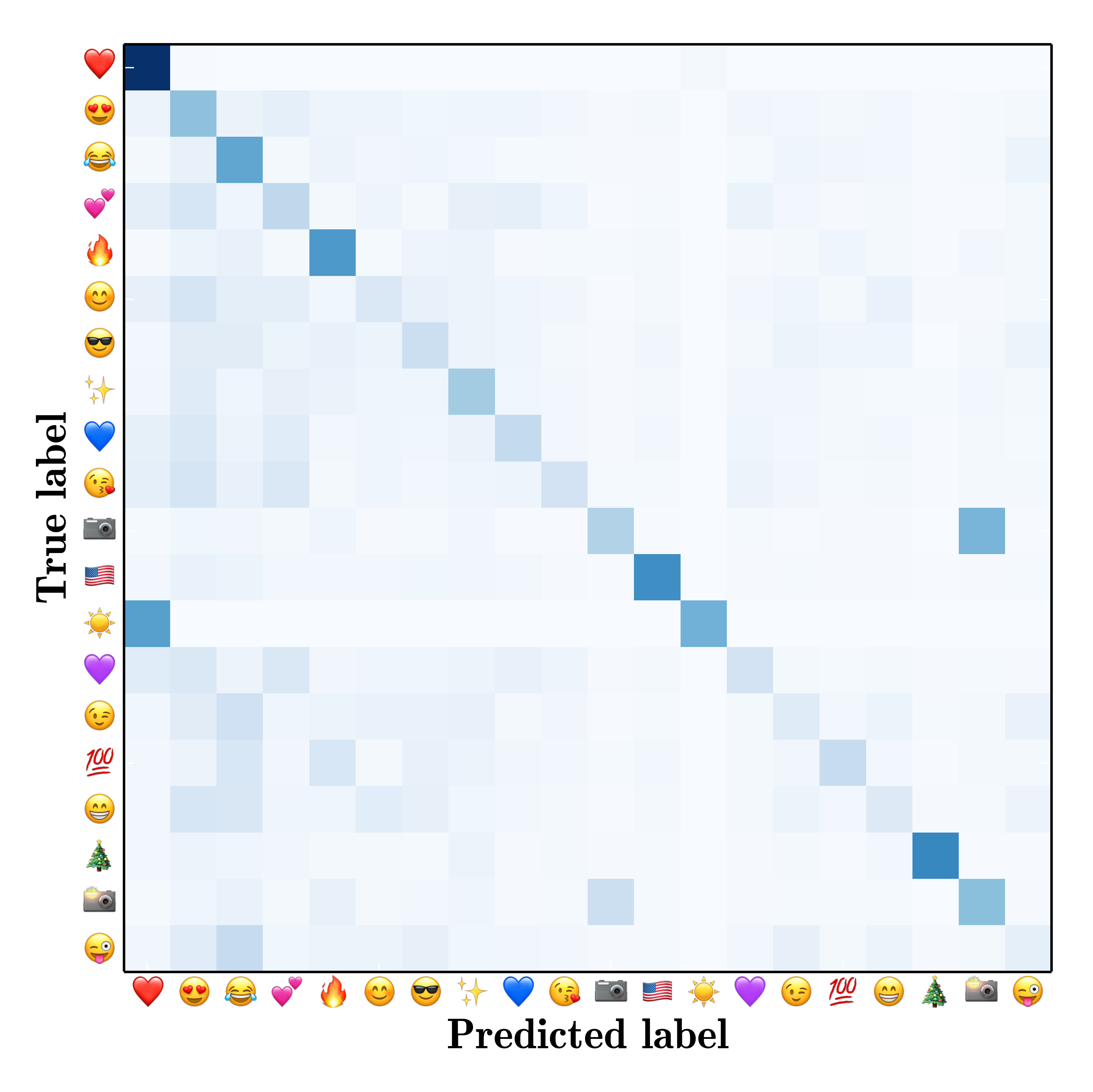
Figure 6: Confusion matrix

Fig. 6 shows the confusion matrix for the $20$ emojis. Observe that our model is more likely to misclassify a rare class as an instance of one of the $4$ more frequent classes, even after the inclusion of class weights in the loss function (Section 4.1). Furthermore, we observe that heart or face emojis, which are more ambiguous, are easily confusable with each other. However, as expected this in not the case for emojis like the US flag or the Christmas tree, as they are tied with specific expressions.

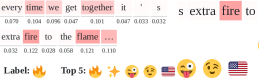
Figure 7: Attention Visualizations

Attention Visualization. The attention mechanism not only improves the performance of the model, but also makes it interpretable. By using the attention scores assigned to each word annotation, we can investigate the behavior of the model. Figure 7 shows how the attention mechanism focuses on each word in order to estimate the most suitable emoji label.

5 Conclusion

In this paper, we present a deep learning system based on a word-level BiLSTM architecture and augment it with contextual attention for SemEval Task 2: “Multilingual Emoji Prediciction” Barbieri et al. (2018). Our work achieved excellent results, reaching the 2nd place in the competition and outperforming the state-of-the-art reported in the bibliography Barbieri et al. (2017). The performance of our model could be further boosted, by utilizing transfer learning methods from larger, weakly annotated, datasets. Moreover, the joint training of word- and character-level models can be tested for further performance improvement.

Finally, we make both our pretrained word embeddings and the source code of our models available to the community, in order to make our results easily reproducible and facilitate further experimentation in the field.

Acknowledgements. This work has been partially supported by the BabyRobot project supported by EU H2020 (grant #687831). Also, the authors would like to thank NVIDIA for supporting this work by donating a TitanX GPU.

References

- Aoki and Uchida (2011) Sho Aoki and Osamu Uchida. 2011. A method for automatically generating the emotional vectors of emoticons using weblog articles. In Proc. 10th WSEAS Int. Conf. on Applied Computer and Applied Computational Science, Stevens Point, Wisconsin, USA, pages 132–136.
- Bahdanau et al. (2014) Dzmitry Bahdanau, Kyunghyun Cho, and Yoshua Bengio. 2014. Neural machine translation by jointly learning to align and translate. CoRR, abs/1409.0473.
- Barbieri et al. (2017) Francesco Barbieri, Miguel Ballesteros, and Horacio Saggion. 2017. Are emojis predictable? In Proceedings of the 15th Conference of the European Chapter of the Association for Computational Linguistics: Volume 2, Short Papers, pages 105–111. Association for Computational Linguistics.
- Barbieri et al. (2018) Francesco Barbieri, Jose Camacho-Collados, Francesco Ronzano, Luis Espinosa-Anke, Miguel Ballesteros, Valerio Basile, Viviana Patti, and Horacio Saggion. 2018. SemEval-2018 Task 2: Multilingual Emoji Prediction. In Proceedings of the 12th International Workshop on Semantic Evaluation (SemEval-2018), New Orleans, LA, United States. Association for Computational Linguistics.
- Barbieri et al. (2016a) Francesco Barbieri, German Kruszewski, Francesco Ronzano, and Horacio Saggion. 2016a. How cosmopolitan are emojis?: Exploring emojis usage and meaning over different languages with distributional semantics. In Proceedings of the 2016 ACM on Multimedia Conference, pages 531–535. ACM.
- Barbieri et al. (2016b) Francesco Barbieri, Francesco Ronzano, and Horacio Saggion. 2016b. What does this emoji mean? a vector space skip-gram model for twitter emojis. In LREC.
- Baziotis et al. (2017) Christos Baziotis, Nikos Pelekis, and Christos Doulkeridis. 2017. Datastories at semeval-2017 task 4: Deep lstm with attention for message-level and topic-based sentiment analysis. In Proceedings of the 11th International Workshop on Semantic Evaluation (SemEval-2017), pages 747–754.
- Bengio et al. (1994) Yoshua Bengio, Patrice Simard, and Paolo Frasconi. 1994. Learning long-term dependencies with gradient descent is difficult. IEEE transactions on neural networks, 5(2):157–166.
- Bergstra et al. (2013) James Bergstra, Daniel Yamins, and David D. Cox. 2013. Making a Science of Model Search: Hyperparameter Optimization in Hundreds of Dimensions for Vision Architectures. ICML (1), 28:115–123.
- Cappallo et al. (2018) Spencer Cappallo, Stacey Svetlichnaya, Pierre Garrigues, Thomas Mensink, and Cees GM Snoek. 2018. The new modality: Emoji challenges in prediction, anticipation, and retrieval. arXiv preprint arXiv:1801.10253.
- Cho et al. (2014) Kyunghyun Cho, Bart Van Merriënboer, Caglar Gulcehre, Dzmitry Bahdanau, Fethi Bougares, Holger Schwenk, and Yoshua Bengio. 2014. Learning phrase representations using RNN encoder-decoder for statistical machine translation. arXiv preprint arXiv:1406.1078.
- Eisner et al. (2016) Ben Eisner, Tim Rocktäschel, Isabelle Augenstein, Matko Bošnjak, and Sebastian Riedel. 2016. emoji2vec: Learning emoji representations from their description. arXiv preprint arXiv:1609.08359.
- Espinosa-Anke et al. (2016) Luis Espinosa-Anke, Horacio Saggion, and Francesco Barbieri. 2016. Revealing patterns of twitter emoji usage in barcelona and madrid. Frontiers in Artificial Intelligence and Applications. 2016;(Artificial Intelligence Research and Development) 288: 239-44.
- Hochreiter et al. (2001) Sepp Hochreiter, Yoshua Bengio, Paolo Frasconi, and Jürgen Schmidhuber. 2001. Gradient Flow in Recurrent Nets: The Difficulty of Learning Long-Term Dependencies. A field guide to dynamical recurrent neural networks. IEEE Press.
- Hochreiter and Schmidhuber (1997) Sepp Hochreiter and Jürgen Schmidhuber. 1997. Long short-term memory. Neural computation, 9(8):1735–1780.
- Jurafsky and James (2000) Daniel Jurafsky and H. James. 2000. Speech and language processing an introduction to natural language processing, computational linguistics, and speech.
- Kingma and Ba (2014) Diederik Kingma and Jimmy Ba. 2014. Adam: A method for stochastic optimization. arXiv preprint arXiv:1412.6980.
- Ljubešić and Fišer (2016) Nikola Ljubešić and Darja Fišer. 2016. A global analysis of emoji usage. In Proceedings of the 10th Web as Corpus Workshop, pages 82–89.
- Mikolov et al. (2013) Tomas Mikolov, Ilya Sutskever, Kai Chen, Greg S. Corrado, and Jeff Dean. 2013. Distributed representations of words and phrases and their compositionality. In Advances in Neural Information Processing Systems, pages 3111–3119.
- Pascanu et al. (2013) Razvan Pascanu, Tomas Mikolov, and Yoshua Bengio. 2013. On the difficulty of training recurrent neural networks. ICML (3), 28:1310–1318.
- Paszke et al. (2017) Adam Paszke, Sam Gross, Soumith Chintala, Gregory Chanan, Edward Yang, Zachary DeVito, Zeming Lin, Alban Desmaison, Luca Antiga, and Adam Lerer. 2017. Automatic differentiation in pytorch.
- Pedregosa et al. (2011) Fabian Pedregosa, Gaël Varoquaux, Alexandre Gramfort, Vincent Michel, Bertrand Thirion, Olivier Grisel, Mathieu Blondel, Peter Prettenhofer, Ron Weiss, Vincent Dubourg, and others. 2011. Scikit-learn: Machine learning in Python. Journal of Machine Learning Research, 12(Oct):2825–2830.
- Řehůřek and Sojka (2010) Radim Řehůřek and Petr Sojka. 2010. Software Framework for Topic Modelling with Large Corpora. In Proceedings of the LREC 2010 Workshop on New Challenges for NLP Frameworks, pages 45–50, Valletta, Malta. ELRA. http://is.muni.cz/publication/884893/en.
- Saggion et al. (2017) Horacio Saggion, Miguel Ballesteros, and Francesco Barbieri. 2017. Are emojis predictable? In EACL.
- Segaran and Hammerbacher (2009) Toby Segaran and Jeff Hammerbacher. 2009. Beautiful Data: The Stories Behind Elegant Data Solutions. "O’Reilly Media, Inc.".
- Srivastava et al. (2014) Nitish Srivastava, Geoffrey E. Hinton, Alex Krizhevsky, Ilya Sutskever, and Ruslan Salakhutdinov. 2014. Dropout: A simple way to prevent neural networks from overfitting. Journal of Machine Learning Research, 15(1):1929–1958.