NTUA-SLP at SemEval-2018 Task 3: Tracking Ironic Tweets using Ensembles of Word and Character Level Attentive RNNs

Abstract

In this paper we present two deep-learning systems that competed at SemEval-2018 Task 3 “Irony detection in English tweets”. We design and ensemble two independent models, based on recurrent neural networks (Bi-LSTM), which operate at the word and character level, in order to capture both the semantic and syntactic information in tweets. Our models are augmented with a self-attention mechanism, in order to identify the most informative words. The embedding layer of our word-level model is initialized with word2vec word embeddings, pretrained on a collection of 550 million English tweets. We did not utilize any handcrafted features, lexicons or external datasets as prior information and our models are trained end-to-end using back propagation on constrained data. Furthermore, we provide visualizations of tweets with annotations for the salient tokens of the attention layer that can help to interpret the inner workings of the proposed models. We ranked 2 out of 42 teams in Subtask A and 2 out of 31 teams in Subtask B. However, post-task-completion enhancements of our models achieve state-of-the-art results ranking 1 for both subtasks.

1 Introduction

Irony is a form of figurative language, considered as saying the opposite of what you mean, where the opposition of literal and intended meanings is very clear Barbieri and Saggion (2014); Liebrecht et al. (2013). Traditional approaches in NLP Tsur et al. (2010); Barbieri and Saggion (2014); Karoui et al. (2015); Farías et al. (2016) model irony based on pattern-based features, such as the contrast between high and low frequent words, the punctuation used by the author, the level of ambiguity of the words and the contrast between the sentiments. Also, Joshi et al. (2016) recently added word embeddings statistics to the feature space and further boosted the performance in irony detection.

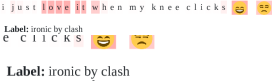
(a)

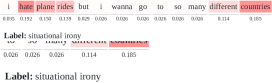
(b)

Figure 1: Attention heat-map visualization. The color intensity of each word / character, corresponds to its weight (importance), as given by the self-attention mechanism (Section 2.6).

Modeling irony, especially in Twitter, is a challenging task, since in ironic comments literal meaning can be misguiding; irony is expressed in “secondary” meaning and fine nuances that are hard to model explicitly in machine learning algorithms. Tracking irony in social media posses the additional challenge of dealing with special language, social media markers and abbreviations. Despite the accuracy achieved in this task by hand-crafted features, a laborious feature-engineering process and domain-specific knowledge are required; this type of prior knowledge must be continuously updated and investigated for each new domain. Moreover, the difficulty in parsing tweets Gimpel et al. (2011) for feature extraction renders their precise semantic representation, which is key of determining their intended gist, much harder.

In recent years, the successful utilization of deep learning architectures in NLP led to alternative approaches for tracking irony in Twitter Joshi et al. (2017); Ghosh and Veale (2017). Ghosh and Veale (2016) proposed a Convolutional Neural Network (CNN) followed by a Long Short Term Memory (LSTM) architecture, outperforming the state-of-the-art. Dhingra et al. (2016) utilized deep learning for representing tweets as a sequence of characters, instead of words and proved that such representations reveal information about the irony concealed in tweets.

In this work, we propose the combination of word- and character-level representations in order to exploit both semantic and syntactic information of each tweet for successfully predicting irony. For this purpose, we employ a deep LSTM architecture which models words and characters separately. We predict whether a tweet is ironic or not, as well as the type of irony in the ironic ones by ensembling the two separate models (late fusion). Furthermore, we add an attention layer to both models, to better weigh the contribution of each word and character towards irony prediction, as well as better interpret the descriptive power of our models. Attention weighting also better addresses the problem of supervising learning on deep learning architectures. The suggested model was trained only on constrained data, meaning that we did not utilize any external dataset for further tuning of the network weights.

The two deep-learning models submitted to SemEval-2018 Task 3 “Irony detection in English tweets” Van Hee et al. (2018) are described in this paper with the following structure: in Section 2 an overview of the proposed models is presented, in Section 3 the models for tracking irony are depicted in detail, in Section 4 the experimental setup alongside with the respective results are demonstrated and finally, in Section 5 we discuss the performance of the proposed models.

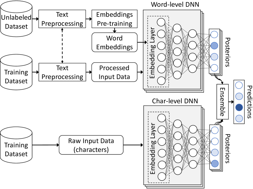
Figure 2: High-level overview of our approach

2 Overview

Fig. 2 provides a high-level overview of our approach, which consists of three main steps: (1) the pre-training of word embeddings, where we train our own word embeddings on a big collection of unlabeled Twitter messages, (2) the independent training of our models: word- and char-level, (3) the ensembling, where we combine the predictions of each model.

2.1 Task definitions

The goal of Subtask A is tracking irony in tweets as a binary classification problem (ironic vs. non-ironic). In Subtask B, we are also called to determine the type of irony, with three different classes of irony on top of the non-ironic one (four-class classification). The types of irony are: (1) Verbal irony by means of a polarity contrast, which includes messages whose polarity (positive, negative) is inverted between the literal and the intended evaluation, such as "I really love this year’s summer; weeks and weeks of awful weather", where the literal evaluation ("I really love this year’s summer") is positive, while the intended one, which is implied in the context ("weeks and weeks of awful weather"), is negative. (2) Other verbal irony, which refers to instances showing no polarity contrast, but are ironic such as "Yeah keeping cricket clean, that’s what he wants #Sarcasm" and (3) situational ironywhich is present in messages that a present situation fails to meet some expectations, such as "Event technology session is having Internet problems. #irony #HSC2024" in which the expectation that a technology session should provide Internet connection is not met.

2.2 Data

Unlabeled Dataset. We collected a dataset of 550 million archived English Twitter messages, from Apr. 2014 to Jun. 2017. This dataset is used for (1) calculating word statistics needed in our text preprocessing pipeline (Section 2.4) and (2) training word2vec word embeddings (Section 2.3).

2.3 Word Embeddings

Word embeddings are dense vector representations of words Collobert and Weston (2008); Mikolov et al. (2013), capturing semantic their and syntactic information. We leverage our unlabeled dataset to train Twitter-specific word embeddings. We use the word2vec  Mikolov et al. (2013) algorithm, with the skip-gram model, negative sampling of 5 and minimum word count of 20, utilizing Gensim’s Řehůřek and Sojka (2010) implementation. The resulting vocabulary contains $800,000$ words. The pre-trained word embeddings are used for initializing the first layer (embedding layer) of our neural networks.

original	The *new* season of #TwinPeaks is coming on May 21, 2017. CANT WAIT \o/ !!! #tvseries #davidlynch :D
processed	the new <emphasis> season of <hashtag> twin peaks </hashtag> is coming on <date> . cant <allcaps> wait <allcaps> <happy> ! <repeated> <hashtag> tv series </hashtag> <hashtag> david lynch </hashtag> <laugh>

Table 1: Example of our text processor

2.4 Preprocessing

We utilized the ekphrasis Baziotis et al. (2017) tool as a tweet preprocessor. The preprocessing steps included in ekphrasis are: Twitter-specific tokenization, spell correction, word normalization, word segmentation (for splitting hashtags) and word annotation.

Tokenization. Tokenization is the first fundamental preprocessing step and since it is the basis for the other steps, it immediately affects the quality of the features learned by the network. Tokenization in Twitter is especially challenging, since there is large variation in the vocabulary and the used expressions. Part of the challenge is also the decision of whether to process an entire expression (e.g. anti-american) or its respective tokens. Ekphrasis overcomes this challenge by recognizing the Twitter markup, emoticons, emojis, expressions like dates (e.g. 07/11/2011, April 23rd), times (e.g. 4:30pm, 11:00 am), currencies (e.g. $10, 25mil, 50€), acronyms, censored words (e.g. s**t) and words with emphasis (e.g. *very*).

Normalization. After the tokenization we apply a series of modifications on the extracted tokens, such as spell correction, word normalization and segmentation. We also decide which tokens to omit, normalize and surround or replace with special tags (e.g. URLs, emails and @user). For the tasks of spell correction Jurafsky and James (2000) and word segmentation Segaran and Hammerbacher (2009) we use the Viterbi algorithm. The prior probabilities are initialized using uni/bi-gram word statistics from the unlabeled dataset.

The benefits of the above procedure are the reduction of the vocabulary size, without removing any words, and the preservation of information that is usually lost during tokenization. Table 1 shows an example text snippet and the resulting preprocessed tokens.

2.5 Recurrent Neural Networks

We model the Twitter messages using Recurrent Neural Networks (RNN). RNNs process their inputs sequentially, performing the same operation, $h_{t}=f_{W}(x_{t},h_{t-1})$, on every element in a sequence, where $h_{t}$ is the hidden state $t$ the time step, and $W$ the network weights. We can see that hidden state at each time step depends on previous hidden states, thus the order of elements (words) is important. This process also enables RNNs to handle inputs of variable length.

RNNs are difficult to train Pascanu et al. (2013), because gradients may grow or decay exponentially over long sequences Bengio et al. (1994); Hochreiter et al. (2001). A way to overcome these problems is to use more sophisticated variants of regular RNNs, like Long Short-Term Memory (LSTM) networks Hochreiter and Schmidhuber (1997) or Gated Recurrent Units (GRU) Cho et al. (2014), which introduce a gating mechanism to ensure proper gradient flow through the network. In this work, we use LSTMs.

2.6 Self-Attention Mechanism

(a) Regular RNN

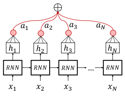
(b) Attention RNN

Figure 3: Comparison between the regular RNN and the RNN with attention.

RNNs update their hidden state $h_{i}$ as they process a sequence and the final hidden state holds a summary of the information in the sequence. In order to amplify the contribution of important words in the final representation, a self-attention mechanism Bahdanau et al. (2014) can be used (Fig. 3). In normal RNNs, we use as representation $r$ of the input sequence its final state $h_{N}$. However, using an attention mechanism, we compute $r$ as the convex combination of all $h_{i}$. The weights $a_{i}$ are learned by the network and their magnitude signifies the importance of each hidden state in the final representation. Formally: $r=\sum_{i=1}^{N}a_{i}h_{i},\mbox{where}\sum_{i=1}^{N}a_{i}=1,\;\mbox{and}\;a_{i}>0.$

3 Models Description

We have designed two independent deep-learning models, with each one capturing different aspects of the tweet. The first model operates at the word-level, capturing the semantic information of the tweet and the second model at the character-level, capturing the syntactic information. Both models share the same architecture, and the only difference is in their embedding layers. We present both models in a unified manner.

3.1 Embedding Layer

Character-level. The input to the network is a Twitter message, treated as a sequence of characters. We use a character embedding layer to project the characters $c_{1},c_{2},...,c_{N}$ to a low-dimensional vector space $R^{C}$, where $C$ the size of the embedding layer and $N$ the number of characters in a tweet. We randomly initialize the weights of the embedding layer and learn the character embeddings from scratch.

Word-level. The input to the network is a Twitter message, treated as a sequence of words. We use a word embedding layer to project the words $w_{1},w_{2},...,w_{N}$ to a low-dimensional vector space $R^{W}$, where $W$ the size of the embedding layer and $N$ the number of words in a tweet. We initialize the weights of the embedding layer with our pre-trained word embeddings.

3.2 BiLSTM Layers

An LSTM takes as input the words (characters) of a tweet and produces the word (character) annotations $h_{1},h_{2},...,h_{N}$, where $h_{i}$ is the hidden state of the LSTM at time-step $i$, summarizing all the information of the sentence up to $w_{i}$ ($c_{i}$). We use bidirectional LSTM (BiLSTM) in order to get word (character) annotations that summarize the information from both directions. A bidirectional LSTM consists of a forward LSTM $\overrightarrow{f}$ that reads the sentence from $w_{1}$ to $w_{N}$ and a backward LSTM $\overleftarrow{f}$ that reads the sentence from $w_{N}$ to $w_{1}$. We obtain the final annotation for a given word $w_{i}$ (character $c_{i}$), by concatenating the annotations from both directions, $h_{i}=\overrightarrow{h_{i}}\parallel\overleftarrow{h_{i}},\quad h_{i}\in R^{2L}$ where $\parallel$ denotes the concatenation operation and $L$ the size of each LSTM. We stack two layers of BiLSTMs in order to learn more high-level (abstract) features.

3.3 Attention Layer

Not all words contribute equally to the meaning that is expressed in a message. We use an attention mechanism to find the relative contribution (importance) of each word. The attention mechanism assigns a weight $a_{i}$ to each word annotation $h_{i}$. We compute the fixed representation $r$ of the whole input message. as the weighted sum of all the word annotations.

$$e_{i} =tanh(W_{h}h_{i}+b_{h}),\quad e_{i}\in[-1,1]$$ (1)

$$a_{i} =\dfrac{exp(e_{i})}{\sum_{t=1}^{T}exp(e_{t})},\quad\sum_{i=1}^{T}a_{i}=1$$ (2)

$$r =\sum_{i=1}^{T}a_{i}h_{i},\quad r\in R^{2L}$$ (3)

where $W_{h}$ and $b_{h}$ are the attention layer’s weights.

Character-level Interpretation. In the case of the character-level model, the attention mechanism operates in the same way as in the word-level model. However, we can interpret the weight given to each character annotation $h_{i}$ by the attention mechanism, as the importance of the information surrounding the given character.

3.4 Output Layer

We use the representation $r$ as feature vector for classification and we feed it to a fully-connected softmax layer with $L$ neurons, which outputs a probability distribution over all classes $p_{c}$ as described in Eq. 4:

$$p_{c}=\frac{e^{Wr+b}}{\sum_{i\in[1,L]}(e^{W_{i}r+b_{i}})}$$ (4)

where $W$ and $b$ are the layer’s weights and biases.

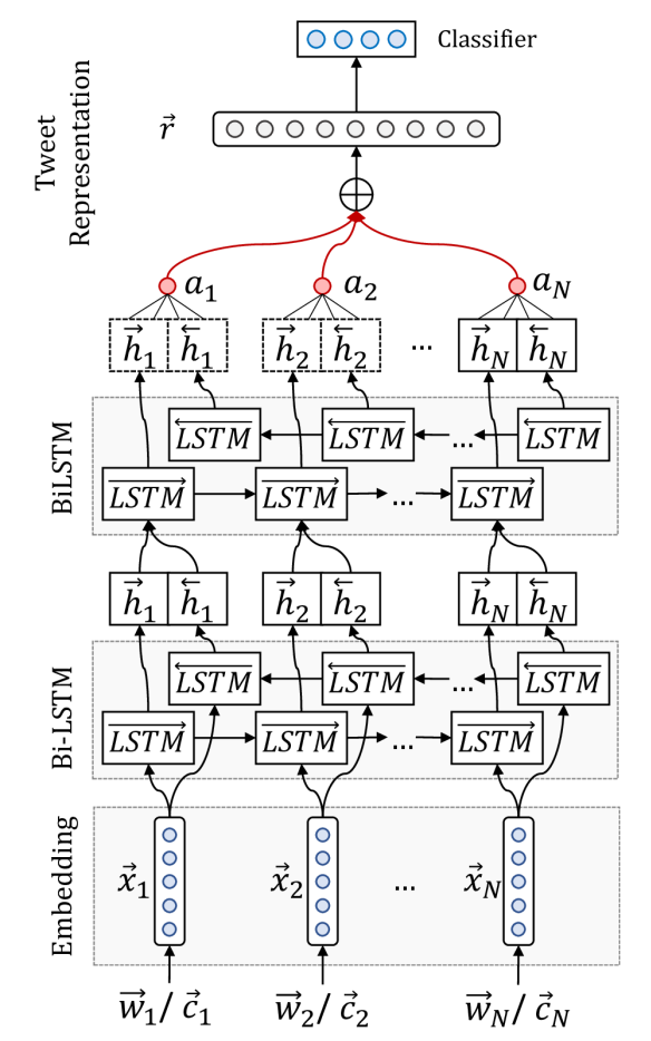
Figure 4: The word/character-level model.

3.5 Regularization

In order to prevent overfitting of both models, we add Gaussian noise to the embedding layer, which can be interpreted as a random data augmentation technique, that makes models more robust to overfitting. In addition to that, we use dropout Srivastava et al. (2014) and early-stopping.

Finally, we do not fine-tune the embedding layers of the word-level model. Words occurring in the training set, will be moved in the embedding space and the classifier will correlate certain regions (in embedding space) to certain meanings or types of irony. However, words in the test set and not in the training set, will remain at their initial position which may no longer reflect their “true” meaning, leading to miss-classifications.

3.6 Ensemble

A key factor to good ensembles, is to utilize diverse classifiers. To this end, we combine the predictions of our word and character level models. We employed two ensemble schemes, namely unweighted average and majority voting.

Unweighted Average (UA). In this approach, the final prediction is estimated from the unweighted average of the posterior probabilities for all different models. Formally, the final prediction $p$ for a training instance is estimated by:

$$p =\operatorname*{arg\,max}_{c}\dfrac{1}{C}\sum_{i=1}^{M}\vec{p_{i}},\quad p_{i}\in{\rm I\!R}^{C}$$ (5)

where $C$ is the number of classes, $M$ is the number of different models, $c\in\{1,...,C\}$ denotes one class and $\vec{p_{i}}$ is the probability vector calculated by model $i\in\{1,...,M\}$ using softmax function.

Majority Voting (MV). Majority voting approach counts the votes of all different models and chooses the class with most votes. Compared to unweighted averaging, MV is affected less by single-network decisions. However, this schema does not consider any information derived from the minority models. Formally, for a task with $C$ classes and $M$ different models, the prediction for a specific instance is estimated as follows:

$$\begin{split}v_{c}&=\sum_{i=1}^{M}F_{i}(c)\\ p&=\operatorname*{arg\,max}_{c\in\{1,...,C\}}v_{c}\end{split}$$ (6)

where $v_{c}$ denotes the votes for class $c$ from all different models, $F_{i}$ is the decision of the $i^{th}$ model, which is either 1 or 0 with respect to whether the model has classified the instance in class $c$ or not, respectively, and $p$ is the final prediction.

4 Experiments and Results

4.1 Experimental Setup

Class Weights. In order to deal with the problem of class imbalances in Subtask B, we apply class weights to the loss function of our models, penalizing more the misclassification of underrepresented classes. We weight each class by its inverse frequency in the training set.

Training We use Adam algorithm Kingma and Ba (2014) for optimizing our networks, with mini-batches of size 32 and we clip the norm of the gradients Pascanu et al. (2013) at 1, as an extra safety measure against exploding gradients. For developing our models we used PyTorch Paszke et al. (2017) and Scikit-learn Pedregosa et al. (2011).

Hyper-parameters. In order to find good hyper-parameter values in a relative short time (compared to grid or random search), we adopt the Bayesian optimization Bergstra et al. (2013) approach, performing a “smart” search in the high dimensional space of all the possible values. Table 2, shows the selected hyper-parameters.

	Word-Model	Char-Model
Embeddings	300	25
Emb. Dropout	0.1	0.0
Emb. Noise	0.05	0.0
LSTM (x2)	150	150
LSTM Dropout	0.2	0.2

Table 2: Hyper-parameters of our models.

4.2 Results and Discussion

Our official ranking is 2/43 in Subtask A and 2/29 in Subtask B as shown in Tables 3 and 4. Based on these rankings, the performance of the suggested model is competitive on both the binary and the multi-class classification problem. Except for its overall good performance, it also presents a stable behavior when moving from two to four classes.

#	Team Name	Acc	Prec	Rec	F1
1	THU_NGN	0.7347	0.6304	0.8006	0.7054
2	NTUA-SLP	0.7321	0.6535	0.6913	0.6719
3	WLV	0.6429	0.5317	0.8360	0.6500
4	Unknown	0.6607	0.5506	0.7878	0.6481
5	NIHRIO, NCL	0.7015	0.6091	0.6913	0.6476

Table 3: Competition results for Subtask A

#	Team Name	Acc	Prec	Rec	F1
1	Unknown	0.7321	0.5768	0.5044	0.5074
2	NTUA-SLP	0.6518	0.4959	0.5124	0.4959
3	THU_NGN	0.6046	0.4860	0.5414	0.4947
4	Unknown	0.6033	0.4660	0.5058	0.4743
5	NIHRIO, NCL	0.6594	0.5446	0.4475	0.4437

Table 4: Competition results for Subtask B

model	Acc	Prec	Rec	f1
BOW	0.6531	0.6453	0.6417	0.6426
N-BOW	0.6645	0.6543	0.6517	0.6527
LSTM-char	0.6241	0.6371	0.6342	0.6163
LSTM-word	0.7746	0.7726	0.7826	0.7698
Ens-MV	0.7462	0.7381	0.7461	0.7400
Ens-UA	0.7883	0.7865	0.7992	0.7856

Table 5: Results of our models for Subtask A

model	Acc	Prec	Rec	f1
BOW	0.5880	0.4460	0.4384	0.4371
N-BOW	0.6084	0.4649	0.4560	0.4520
LSTM-char	0.5726	0.4098	0.4102	0.3782
LSTM-word	0.6987	0.5394	0.5790	0.5315
Ens-MV	0.6888	0.5433	0.5442	0.5358
Ens-UA	0.6888	0.5361	0.4874	0.4959

Table 6: Results of our models for Subtask B

Additional experimentation following the official submission significantly improved the efficiency of our models. The results of this experimentation, tested on the same data set, are shown in Tables 5 and 6. The first baseline is a Bag of Words (BOW) model with TF-IDF weighting. The second baseline is a Neural Bag of Words (N-BOW) model where we retrieve the word2vec representations of the words in a tweet and compute the tweet representation as the centroid of the constituent word2vec representations. Both BOW and N-BOW features are then fed to a linear SVM classifier, with tuned $C=0.6$.

The best performance that we achieve, as shown in Tables 5 and 6 is 0.7856 and 0.5358 for Subtask A and B respectively. In Subtask A the BOW and N-BOW models perform similarly with respect to f1 metric and word-level LSTM is the most competitive individual model. However, the best performance is achieved when the character- and the word-level LSTM models are combined via the unweighted average ensembling method, showing that the two suggested models indeed contain different types of information related to irony on tweets. Similar observations are derived for Subtask B, except that the character-level model in this case performs worse than the baseline models and contributes less to the final results.

(a)

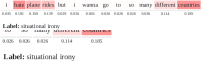
(b)

(c)

Figure 5: Examples of the attention mechanism for identification of the type of irony in each sentence.

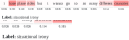
Figure 6: Comparison of the behavior of the word and character level models.

4.3 Attention Visualizations

Our models’ behavior can be interpreted by visualizing the distribution of the attention weights assigned to the words (characters) of the tweet. The weights signify the contribution of each word (character), to model’s final classification decision. In Fig. 5, examples of the weights assigned by the word level model to ironic tweets are presented. The salient keywords that capture the essence of irony or even polarity transitions (e.g. irony by clash) are correctly identified by the model. Moreover, in Fig. 6 we compare the behavior of the word and character models on the same tweets. In the first example, the character level model assigns larger weights to the most discriminative words whereas the weights assigned by the word level model seem uniform and insufficient in spotting the polarity transition. However, in the second example, the character level model does not attribute any weight to the words with positive polarity (e.g. “fun”) compared to the word level model. Based on these observations, the two models indeed behave diversely and consequently contribute to the final outcome (see Section 3.6).

5 Conclusion

In this paper we present an ensemble of two different deep learning models: a word- and a character-level deep LSTM for capturing the semantic and syntactic information of tweets, respectively. We demonstrated that combining the predictions of the two models yields competitive results in both subtasks for irony prediction. Moreover, we proved that both types of information (semantic and syntactic) contribute to the final results with the word-level model, however, individually achieving more accurate irony prediction. Also, the best way of combining the outcomes of the separate models is by conducting majority voting over the respective posteriors. Finally, the proposed model successfully predicts the irony in tweets without exploiting any external information derived from hand-crafted features or lexicons.

The performance reported in this paper could be further boosted by utilizing transfer learning methods from larger datasets. Moreover, the joint training of word- and character-level models can be tested for further improvement of the results. Finally, we make the source code of our models and our pretrained word embeddings available to the community, in order to make our results easily reproducible and facilitate further experimentation.

Acknowledgements. This work has been partially supported by the BabyRobot project supported by EU H2020 (grant #687831). Also, the authors would like to thank NVIDIA for supporting this work by donating a TitanX GPU.

References

- Bahdanau et al. (2014) Dzmitry Bahdanau, Kyunghyun Cho, and Yoshua Bengio. 2014. Neural machine translation by jointly learning to align and translate. CoRR, abs/1409.0473.
- Barbieri and Saggion (2014) Francesco Barbieri and Horacio Saggion. 2014. Automatic detection of irony and humour in twitter. In ICCC, pages 155–162.
- Baziotis et al. (2017) Christos Baziotis, Nikos Pelekis, and Christos Doulkeridis. 2017. Datastories at semeval-2017 task 4: Deep lstm with attention for message-level and topic-based sentiment analysis. In Proceedings of the 11th International Workshop on Semantic Evaluation (SemEval-2017), pages 747–754.
- Bengio et al. (1994) Yoshua Bengio, Patrice Simard, and Paolo Frasconi. 1994. Learning long-term dependencies with gradient descent is difficult. IEEE transactions on neural networks, 5(2):157–166.
- Bergstra et al. (2013) James Bergstra, Daniel Yamins, and David D. Cox. 2013. Making a Science of Model Search: Hyperparameter Optimization in Hundreds of Dimensions for Vision Architectures. ICML (1), 28:115–123.
- Cho et al. (2014) Kyunghyun Cho, Bart Van Merriënboer, Caglar Gulcehre, Dzmitry Bahdanau, Fethi Bougares, Holger Schwenk, and Yoshua Bengio. 2014. Learning phrase representations using RNN encoder-decoder for statistical machine translation. arXiv preprint arXiv:1406.1078.
- Collobert and Weston (2008) Ronan Collobert and Jason Weston. 2008. A unified architecture for natural language processing: Deep neural networks with multitask learning. In Proceedings of the 25th International Conference on Machine Learning, pages 160–167. ACM.
- Dhingra et al. (2016) Bhuwan Dhingra, Zhong Zhou, Dylan Fitzpatrick, Michael Muehl, and William W Cohen. 2016. Tweet2vec: Character-based distributed representations for social media. arXiv preprint arXiv:1605.03481.
- Farías et al. (2016) Delia Irazú Hernańdez Farías, Viviana Patti, and Paolo Rosso. 2016. Irony detection in twitter: The role of affective content. ACM Transactions on Internet Technology (TOIT), 16(3):19.
- Ghosh and Veale (2016) Aniruddha Ghosh and Tony Veale. 2016. Fracking sarcasm using neural network. In Proceedings of the 7th Workshop on Computational Approaches to Subjectivity, Sentiment and Social Media Analysis, pages 161–169.
- Ghosh and Veale (2017) Aniruddha Ghosh and Tony Veale. 2017. Magnets for sarcasm: Making sarcasm detection timely, contextual and very personal. In Proceedings of the 2017 Conference on Empirical Methods in Natural Language Processing, pages 482–491.
- Gimpel et al. (2011) Kevin Gimpel, Nathan Schneider, Brendan O’Connor, Dipanjan Das, Daniel Mills, Jacob Eisenstein, Michael Heilman, Dani Yogatama, Jeffrey Flanigan, and Noah A. Smith. 2011. Part-of-speech tagging for twitter: Annotation, features, and experiments. In Proceedings of the 49th Annual Meeting of the Association for Computational Linguistics: Human Language Technologies: Short Papers-Volume 2, pages 42–47. Association for Computational Linguistics.
- Hochreiter et al. (2001) Sepp Hochreiter, Yoshua Bengio, Paolo Frasconi, and Jürgen Schmidhuber. 2001. Gradient Flow in Recurrent Nets: The Difficulty of Learning Long-Term Dependencies. A field guide to dynamical recurrent neural networks. IEEE Press.
- Hochreiter and Schmidhuber (1997) Sepp Hochreiter and Jürgen Schmidhuber. 1997. Long short-term memory. Neural computation, 9(8):1735–1780.
- Joshi et al. (2017) Aditya Joshi, Pushpak Bhattacharyya, and Mark J Carman. 2017. Automatic sarcasm detection: A survey. ACM Computing Surveys (CSUR), 50(5):73.
- Joshi et al. (2016) Aditya Joshi, Vaibhav Tripathi, Kevin Patel, Pushpak Bhattacharyya, and Mark Carman. 2016. Are word embedding-based features useful for sarcasm detection? arXiv preprint arXiv:1610.00883.
- Jurafsky and James (2000) Daniel Jurafsky and H. James. 2000. Speech and language processing an introduction to natural language processing, computational linguistics, and speech.
- Karoui et al. (2015) Jihen Karoui, Farah Benamara, Véronique Moriceau, Nathalie Aussenac-Gilles, and Lamia Hadrich Belguith. 2015. Towards a contextual pragmatic model to detect irony in tweets. In 53rd Annual Meeting of the Association for Computational Linguistics (ACL 2015), pages PP–644.
- Kingma and Ba (2014) Diederik Kingma and Jimmy Ba. 2014. Adam: A method for stochastic optimization. arXiv preprint arXiv:1412.6980.
- Liebrecht et al. (2013) CC Liebrecht, FA Kunneman, and APJ van Den Bosch. 2013. The perfect solution for detecting sarcasm in tweets# not.
- Mikolov et al. (2013) Tomas Mikolov, Ilya Sutskever, Kai Chen, Greg S. Corrado, and Jeff Dean. 2013. Distributed representations of words and phrases and their compositionality. In Advances in Neural Information Processing Systems, pages 3111–3119.
- Pascanu et al. (2013) Razvan Pascanu, Tomas Mikolov, and Yoshua Bengio. 2013. On the difficulty of training recurrent neural networks. ICML (3), 28:1310–1318.
- Paszke et al. (2017) Adam Paszke, Sam Gross, Soumith Chintala, Gregory Chanan, Edward Yang, Zachary DeVito, Zeming Lin, Alban Desmaison, Luca Antiga, and Adam Lerer. 2017. Automatic differentiation in pytorch.
- Pedregosa et al. (2011) Fabian Pedregosa, Gaël Varoquaux, Alexandre Gramfort, Vincent Michel, Bertrand Thirion, Olivier Grisel, Mathieu Blondel, Peter Prettenhofer, Ron Weiss, Vincent Dubourg, and others. 2011. Scikit-learn: Machine learning in Python. Journal of Machine Learning Research, 12(Oct):2825–2830.
- Řehůřek and Sojka (2010) Radim Řehůřek and Petr Sojka. 2010. Software Framework for Topic Modelling with Large Corpora. In Proceedings of the LREC 2010 Workshop on New Challenges for NLP Frameworks, pages 45–50, Valletta, Malta. ELRA. http://is.muni.cz/publication/884893/en.
- Segaran and Hammerbacher (2009) Toby Segaran and Jeff Hammerbacher. 2009. Beautiful Data: The Stories Behind Elegant Data Solutions. "O’Reilly Media, Inc.".
- Srivastava et al. (2014) Nitish Srivastava, Geoffrey E. Hinton, Alex Krizhevsky, Ilya Sutskever, and Ruslan Salakhutdinov. 2014. Dropout: A simple way to prevent neural networks from overfitting. Journal of Machine Learning Research, 15(1):1929–1958.
- Tsur et al. (2010) Oren Tsur, Dmitry Davidov, and Ari Rappoport. 2010. Icwsm-a great catchy name: Semi-supervised recognition of sarcastic sentences in online product reviews. In ICWSM, pages 162–169.
- Van Hee et al. (2018) Cynthia Van Hee, Els Lefever, and Véronique Hoste. 2018. SemEval-2018 Task 3: Irony Detection in English Tweets. In Proceedings of the 12th International Workshop on Semantic Evaluation, SemEval-2018, New Orleans, LA, USA. Association for Computational Linguistics.
- Wilson and Schakel (2015) Benjamin J Wilson and Adriaan MJ Schakel. 2015. Controlled experiments for word embeddings. arXiv preprint arXiv:1510.02675.