Charge self-consistent many-body corrections using optimized projected localized orbitals

Abstract

In order for methods combining ab-initio density-functional theory and many-body techniques to become routinely used, a flexible, fast, and easy-to-use implementation is crucial. We present an implementation of a general charge self-consistent scheme based on projected localized orbitals in the Projector Augmented Wave framework in the Vienna Ab-Initio Simulation Package (vasp). We give a detailed description on how the projectors are optimally chosen and how the total energy is calculated. We benchmark our implementation in combination with dynamical mean-field theory: First we study the charge-transfer insulator NiO using a Hartree-Fock approach to solve the many-body Hamiltonian. We address the advantages of the optimized against non-optimized projectors and furthermore find that charge self-consistency decreases the dependence of the spectral function – especially the gap – on the double counting. Second, using continuous-time quantum Monte Carlo we study a monolayer of SrVO₃, where strong orbital polarization occurs due to the reduced dimensionality. Using total-energy calculation for structure determination, we find that electronic correlations have a non-negligible influence on the position of the apical oxygens, and therefore on the thickness of the single SrVO₃ layer.

1 Introduction

The advances in the field of nanostructures, where control is now experimentally possible on an atom-by-atom scale, have given rise to a strong demand for theoretical simulation tools that are capable of simulating complex correlated electron systems such as heterostructures, clusters, or adatom arrays on surfaces. There are several successful approaches that can be used for that. Among the most widely used are ab-initio approaches, notably density functional theory (DFT) and many-body model Hamiltonians.

Modern Kohn-Sham DFT, within the local density approximation (LDA) [1] or a generalized gradient approximation (GGA) [2], yields various ground-state properties including crystal structures quite reliably for many materials, essentially without any ambiguous input parameters. The auxiliary single-particle energies can be seen as an estimate of the electronic quasi-particle energies,[3] sometimes giving good qualitative agreement. However, (semi)local functionals like LDA or GGA are well known to fail to capture the physics of strongly-correlated materials such as Mott insulators, unconventional superconductors, heavy Fermion systems, or Kondo systems.

This is why, for treating these systems, model Hamiltonians such as the Hubbard model are usually employed. Generally speaking, these approaches focus on the description of electron correlation phenomena in a minimal low-energy Hilbert space. They are accessible by a broad set of many-body techniques including dynamical mean-field theory (DMFT)[4] and generalizations thereof. These models naturally depend on model parameters that are unknown a priori. Keeping the number of parameters low can lead to over-simplified models that fail to explain sufficiently well experimental findings. On the other hand, keeping a large number of unknown parameters makes the results ambiguous already from the outset.

Therefore, to obtain the best of both worlds, it appears natural to combine the complementary strengths of both approaches to model correlated electron systems in a realistic manner. To achieve this goal, there has been an ongoing effort in the development of approaches like DFT+DMFT[5, 6] for more than 20 years now. The class of materials addressed by DFT+DMFT is very wide and includes Mott insulators, correlated metals, superconductors, and magnetic materials.

On the DFT side, simulations using projector augmented wave (PAW) [7] basis sets turn out to provide a good compromise between accuracy and computational requirements in these systems. Thus, several DFT+DMFT approaches have been implemented with PAW basis sets on the DFT side.[8, 9] In its most simple formulation, the DMFT is performed on top of a converged DFT calculation (so-called one-shot DFT+DMFT). For many systems, especially those where the strong correlations cause a rearrangement of charges, the success of the method can be significantly improved by performing a fully charge self-consistent calculation. [10, 11, 12, 13, 14] There, the electron density obtained from the DMFT calculation is fed back to the DFT code and the entire loop is self-consistently solved. There already exist implementations of DFT+DMFT using the PAW formalism that include charge self-consistency. [15, 16, 17]

Here we describe a fully charge self-consistent implementation based on optimized projected local orbitals in the Vienna Ab Initio Simulation Package (vasp).[18, 19, 20] On the DFT side, it is flexible and easy to use; vasp provides the data necessary to construct the low-energy model of the system and offers an interface so that the updated charge density can be handed back. This makes it possible to combine it, e.g., with any kind of many-body correction beyond DFT in some correlated subspace defined via local projection operators without requiring any changes to the DFT code. On the DMFT side, we present two codes making use of this extension of vasp.

The paper is organized as follows. In section 2 we explain the details of our approach, particularly, the definition of the optimized local projectors and the way the charge feedback from the many-body to the DFT part is implemented. We then present an application to the testbed material of NiO in section 3, where we first analyze the optimized versus non-optimized projectors and second demonstrate how full charge self-consistency affects simulations of the electronic structure, particularly, in relation with the so-called double-counting problem. In section 4, we report an application of our scheme to monolayers of SrVO₃, where we compare our implementation, in the triqs[21] framework, to the already existing interface between triqs and the DFT code wien2k.[22, 23] Furthermore, for that material, we demonstrate total energy calculations and find structural changes induced by correlations.

2 Details of the implementation

2.1 Correlated subspace from optimally projected local orbitals

To perform DFT+DMFT calculations one needs a way to transform between the basis of the Kohn-Sham (KS) states and the localized basis of the subspace used to define lattice models, e.g., a Hubbard model. The most obvious way to do this is to perform a unitary transformation of a subset of KS states to construct a set of local states. This method is at the heart of various types of Wannier function based methods, such as the maximally-localized Wannier functions.[24]

In many cases, when KS bands with different characters are strongly entangled, it becomes however difficult to construct a well-defined unitary transformation. In this case it is more advantageous to use projector operators which, acting on the KS Hilbert space, project out only KS states with a desired character. This is the basis of projected localized orbitals (PLO).[8]

In the PLO formalism one starts by defining an orthonormal localized basis set $|{\chi_{L}}\rangle$ associated with each correlated site, which is typically indexed by local quantum numbers, e.g., $L=\{l,m,\sigma,...\}$ with ($l,m$) and $\sigma$ being orbital and spin angular-momentum quantum-numbers, respectively. $\{|{\chi_{L}}\rangle\}$ spans a correlated subspace $\mathcal{C}$ at each correlated site. Assuming $\langle{\chi_{L}}|{\chi_{L^{\prime}}}\rangle=\delta_{LL^{\prime}}$, any operator acting on this space can be constructed by projecting onto $\mathcal{C}{}$ using a projector operator $\hat{P}^{\mathcal{C}}$, i.e.,

$$\hat{A}^{\mathrm{imp}}=\hat{P}^{\mathcal{C}}\hat{A}\hat{P}^{\mathcal{C}},$$ (1)

$$\hat{P}^{\mathcal{C}}=\sum_{L}|{\chi_{L}}\rangle\langle{\chi_{L}}|.$$ (2)

An arbitrary vector $|{\Psi}\rangle$ of the Hilbert space can be decomposed in terms of local states by writing $\hat{P}^{\mathcal{C}}|{\Psi}\rangle=\sum_{L}|{\chi_{L}}\rangle\langle{\chi_{L}}|{\Psi}\rangle$. If we now consider a complete basis $|{\Psi_{\mu}}\rangle$, the projector operator is completely defined by specifying PLO functions $P_{L,\mu}\equiv\langle{\chi_{L}}|{\Psi_{\mu}}\rangle$.

As described in detail in [8, 9], the PLO projector in the PAW framework[7, 18] can be written as

$$P^{\mathbf{R}}_{L,\nu}(\mathbf{k})=\sum_{i}\langle{\chi_{L}^{\mathbf{R}}}|{\phi_{i}}\rangle\langle{\tilde{p}_{i}}|{\tilde{\Psi}_{\nu\mathbf{k}}}\rangle,$$ (3)

where $|{\chi_{L}^{\mathbf{R}}}\rangle$ are localized basis functions associated with each correlated site ${\mathbf{R}}$, $|{{\phi_{i}}}\rangle$ are all-electron partial waves, and $|{\tilde{p}_{i}}\rangle$ are the standard PAW projectors. In the following, we will omit the site index $\mathbf{R}$ unless it leads to a confusion. The index $i$ stands for the PAW channel $n$, the angular momentum quantum number $l$, and its magnetic quantum number $m$. $|{\tilde{\Psi}_{\nu\mathbf{k}}}\rangle$ are pseudo-KS states. For the PAW potentials distributed with vasp, generally a minimum of two channels $n$ for each angular quantum number are used. For instance for $3d$ elements, the first $3d$ channel is placed at the energy of the bound $3d$ state in the atom, and a second channel is added a few eV above the bound atomic $3d$ state. Inclusion of the second channel improves the transferability of the PAW potentials and the description of the scattering properties greatly. For $s$ and $p$ states in, e.g., $3d$ transition metals, the first channel usually describes $3s$ and $3p$ semi-core states and the second channel is placed somewhere in the valence regime ($4s$ and $4p$ states) or even above the vacuum level. Although a description of how the projectors have been obtained is stored in more recent PAW potential files, it is not always straightforward for the user to identify the best suitable PLO projectors.

Specifically, various choices are possible for $|{\chi_{L}}\rangle$.[9] Conveniently, one might simply use the all-electron partial waves for a particular PAW channel $n$, $|{\phi_{Ln}}\rangle$, as the local basis. However, doing so in vasp can lead to a non-optimal projection. For instance, for transition metals to the left of the periodic table, the $d$ states in the solid might be more or less contracted than those in the atom, so that the “best” $|{\chi_{L}}\rangle$ is a linear combination of the two available $3d$ channels. Likewise, projection onto the TM valence $s$ states is often difficult, because of the presence of semi-core $s$ states in the PAW potential file. Ideally, the user should not need to make a manual choice of the local $|{\chi_{L}}\rangle$ functions.

In the following we explain a protocol that largely resolves these issues. The first step is not strictly required, but simplifies the subsequent coding somewhat. We first construct a set of PAW projectors and partial waves that are orthogonalized inside the PAW sphere. This can be achieved by diagonalizing the all-electron one-center overlap matrix $O_{nn^{\prime}}$ (for each angular and magnetic quantum number $L$),

$$O_{nn^{\prime}}=\langle{\phi_{Ln}}|{\phi_{Ln^{\prime}}}\rangle,$$ (4)

which gives the eigenvalues $\lambda_{n}$ and the eigenvector matrix $U$,

$$\Lambda=\mathrm{diag}(\lambda_{1},\dots,\lambda_{n}),$$ (5)

$$\Lambda=U^{\dagger}OU.$$ (6)

The new partial waves and the corresponding PAW projectors can now be defined as linear combinations of the original ones:

$$|{\xi_{Ln}}\rangle=\frac{1}{\sqrt{\lambda_{n}}}\sum_{n^{\prime}}U_{nn^{\prime}}|{\phi_{Ln^{\prime}}}\rangle,$$ (7)

$$\langle{\tilde{\beta}_{Ln}}|=\sqrt{\lambda_{n}}\sum_{n^{\prime}}U^{\dagger}_{n^{\prime}n}\langle{\tilde{p}_{Ln^{\prime}}}|.$$ (8)

This new set of projectors and partial waves have the important property that the all-electron partial waves $|{\xi_{Ln}}\rangle$ are orthogonal to each other and that they are normalized to one. Thus, we will now refer to them as “orthonormal” partial waves. The choice above is not unique, though, for instance one might also adopt a Gram-Schmidt orthogonalization procedure.

To construct a unique projector, we seek a unitary transformation that maximizes the overlap between the projector and KS valence states within a chosen (user supplied) energy window $[\varepsilon^{P}_{\min},\varepsilon^{P}_{\max}]$. Specifically, we diagonalize a matrix

$$M_{nn^{\prime}}=\sum_{\nu\mathbf{k}}\langle{\tilde{\beta}_{Ln}}|{\tilde{\Psi}_{\nu\mathbf{k}}}\rangle\langle{\tilde{\Psi}_{\nu\mathbf{k}}}|{\tilde{\beta}_{Ln^{\prime}}}\rangle,$$ (9)

where the sum is restricted to states with energies $\varepsilon_{\nu\mathbf{k}}\in[\varepsilon^{P}_{\min},\varepsilon^{P}_{\max}]$. We then pick the eigenvector $\upsilon_{n}$ with the largest absolute eigenvalue to construct local basis functions and corresponding PAW projectors,

$$|{\chi_{L}}\rangle=\sum_{n}\upsilon_{n}|{\xi_{Ln}}\rangle,$$ (10)

$$\langle{\tilde{\pi}_{L}}|=\sum_{n}\upsilon^{*}_{n}\langle{\tilde{\beta}_{Ln}}|,$$ (11)

with projector functions given by

$$P_{L,\nu}(\mathbf{k})=\langle{\tilde{\pi}_{L}}|{\tilde{\Psi}_{\nu\mathbf{k}}}\rangle.$$ (12)

We note in passing that both steps could be combined into a single computational step, by diagonalization of a generalized eigenvalue problem involving the overlap matrix $O$ and the matrix $M$ evaluated using the original set of projectors and partial waves.

Note that since the all-electron partial waves do not form an orthonormal basis set between different PAW spheres and because projection is performed for a subset of KS states, the above procedure will usually produce non-normalized local states. However, normalized local states can be constructed if we orthonormalize the projector functions as follows,

$$O_{LL^{\prime}}=\sum_{\nu\mathbf{k}}P_{L,\nu}(\mathbf{k})P^{*}_{\nu,L^{\prime}}(\mathbf{k}),$$ (13)

$$P_{L,\nu}(\mathbf{k})\leftarrow\sum_{L^{\prime}}O_{LL^{\prime}}^{-\frac{1}{2}}P_{L^{\prime},\nu}(\mathbf{k}).$$ (14)

On a technical level, the optimal projectors are constructed internally in vasp according to (4-12) for each sites $\mathbf{R}$ given an energy window $[\varepsilon^{P}_{\min},\varepsilon^{P}_{\max}]$. The last orthonormalization step (14) is done externally as post-processing. This allows one to choose a different energy window for the summation in (13) in order to fine-tune the degree of localization of the impurity Wannier functions.

The projection scheme has been used quite widely in the solid state community,[8, 9] even in combination with VASP. When using VASP, these calculations were often not based on a solid mathematical foundation. VASP used to project onto all available PAW projectors with a certain angular and momentum quantum number $lm$, summed the resulting densities, averaged the phase factors and intensities over all $lm$ projectors, and finally wrote the results to a file (PROCAR). Such a prescription, in particular, the averaging of the intensities and phase factors was done ad hoc without a proper mathematical prescription. This can result in unsatisfactory results if the two projectors span a completely different subspace, for instance Ni $3d$ and $4d$ states, or transition metal semi-core $p$ states and valence $p$ states. We will demonstrate this issue for NiO in section 3.1.

2.2 Total energy and charge self-consistency

A general extension of DFT Kohn-Sham equations to a many-body problem based on the Hubbard model can be formulated using the total-energy functional[25, 10]

$$\eqalign{E[n,&{\hat{G}}^{\mathcal{C}}]=\frac{1}{\beta}\sum_{\rmi\omega_{n}\mathbf{k}}\Tr\{\hat{G}(\mathbf{k},\rmi\omega_{n})\hat{H}_{\mathtt{KS}}(\mathbf{k})\}\\ &+E_{H}[n]+E_{\mathrm{xc}}[n]-\int d\mathbf{r}\,(v_{\mathrm{xc}}+v_{H})n(\mathbf{r})\\ &+E_{\mathrm{corr}}[{\hat{G}}^{\mathcal{C}}]-E_{\textsc{dc}}[{\hat{G}}^{\mathcal{C}}],}$$ (18)

where ${\hat{G}}(\mathbf{k},\rmi\omega_{n})$ is the Green’s function containing many-body effects, and $\hat{H}_{\mathtt{KS}}(\mathbf{k})=\sum_{\nu}|{\Psi_{\nu\mathbf{k}}}\rangle\varepsilon_{\nu\mathbf{k}}\langle{\Psi_{\nu\mathbf{k}}}|$ is the KS Hamiltonian. The charge density, $n(\mathbf{r})$, and Green’s function in the correlated subspace, ${\hat{G}}^{\mathcal{C}}(\mathbf{k},\rmi\omega_{n})$, are both related to $\hat{G}(\mathbf{k},\rmi\omega_{n})$ by

$$n(\mathbf{r})=\frac{1}{\beta}\Tr\sum_{\rmi\omega_{n}\mathbf{k}}\langle{\mathbf{r}}|{\hat{G}(\mathbf{k},\rmi\omega_{n})}|{\mathbf{r}}\rangle,$$ (19)

$${\hat{G}}^{\mathcal{C}}(\mathbf{k},\rmi\omega_{n})=\hat{P}^{\mathcal{C}}(\mathbf{k})\hat{G}(\mathbf{k},\rmi\omega_{n})\hat{P}^{\mathcal{C}}(\mathbf{k}),$$ (20)

where $\hat{P}^{\mathcal{C}}_{\mathbf{k}}$ projects onto correlated localized states, see (2). $E_{\mathrm{corr}}$ is the energy contribution of the interaction term (Hubbard $U$-term) and $E_{\textsc{dc}}$ is the double-counting correction.

The first four terms of the above expression form the usual DFT total energy calculated for the density matrix and charge density of the interacting system, which is non-diagonal in this case. It is thus clear that to get the correct value of the total energy the density matrix must be calculated in a self-consistent manner.

In the framework of DFT+DMFT [4, 6] the interacting Green’s function is defined as follows:

$$\hat{G}(\mathbf{k},\rmi\omega_{n})=\left[(\rmi\omega_{n}+\mu)\hat{1\!\!1}-\hat{H}_{\mathtt{KS}}(\mathbf{k})-\hat{\Sigma}^{\mathtt{KS}}(\mathbf{k},\rmi\omega_{n})\right]^{-1},$$ (21)

where $\hat{\Sigma}^{\mathtt{KS}}(\mathbf{k},\rmi\omega_{n})$ is obtained by up-folding the local self-energy,

$$\eqalign{\hat{\Sigma}^{\mathtt{KS}}(\mathbf{k},\rmi\omega_{n})=&\sum_{\nu\nu^{\prime}}|{\Psi_{\nu\mathbf{k}}}\rangle\langle{\Psi_{\nu^{\prime}\mathbf{k}}}|\\ &\cdot\sum_{mm^{\prime}}P^{*}_{\nu,m}(\mathbf{k})\Sigma_{mm^{\prime}}(\rmi\omega_{n})P_{m^{\prime},\nu^{\prime}}(\mathbf{k}),}$$ (24)

where the local self energy’s matrix elements in the basis of localized impurity states, $|{\chi_{lm}}\rangle$, are

$$\Sigma_{mm^{\prime}}(\rmi\omega_{n})=\Sigma^{\mathrm{imp}}_{mm^{\prime}}(\rmi\omega_{n})-\Sigma^{\textsc{dc}}_{mm^{\prime}},$$ (25)

which consist of the purely local impurity self-energy $\hat{\Sigma}^{\mathrm{imp}}(\rmi\omega_{n})$, obtained from an impurity solver, and the double counting $\hat{\Sigma}^{\textsc{dc}}$. Using the PLO functions we can write this Green’s function in terms of its KS matrix elements

$$\eqalign{G_{\nu\nu^{\prime}}(\mathbf{k},\rmi\omega_{n})=\Big{[}(\rmi\omega_{n}+&\mu-\varepsilon_{\nu\mathbf{k}})\hat{1\!\!1}\\ &-\hat{\Sigma}^{\mathtt{KS}}(\mathbf{k},\rmi\omega_{n})\Big{]}^{-1}_{\nu\nu^{\prime}}.}$$ (28)

If we define an energy window $[\varepsilon^{C}_{\min},\varepsilon^{C}_{\max}]$ which selects a subset $\mathcal{W}^{C}$ of KS states affected by correlations, the interacting charge density can be written as

$$\eqalign{n(\mathbf{r})&=\sum_{\mathbf{k}}\sum_{\nu\notin\mathcal{W}^{C}}f_{\nu\mathbf{k}}\langle{\mathbf{r}}|{\Psi_{\nu\mathbf{k}}}\rangle\langle{\Psi_{\nu\mathbf{k}}}|{\mathbf{r}}\rangle\\ &+\sum_{\mathbf{k}}\sum_{\nu\nu^{\prime}\in\mathcal{W}^{C}}\langle{\mathbf{r}}|{\Psi_{\nu\mathbf{k}}}\rangle N_{\nu\nu^{\prime}}(\mathbf{k})\langle{\Psi_{\nu^{\prime}\mathbf{k}}}|{\mathbf{r}}\rangle,}$$ (31)

where we use a non-diagonal density matrix

$$N_{\nu\nu^{\prime}}(\mathbf{k})= \frac{1}{\beta}\sum_{\rmi\omega_{n}}G_{\nu\nu^{\prime}}(\mathbf{k},\rmi\omega_{n}),$$ (32)

and a diagonal density matrix formed by the KS occupation numbers $f_{\nu\mathbf{k}}$. Note that the chemical potential $\mu$ here is generally different from the KS chemical potential $\mu_{\mathtt{KS}}$. The subset of KS states for the optimization of the projectors $\mathcal{W}^{P}$ and KS states affected by correlations $\mathcal{W}^{C}$ can be chosen to be the same but one does necessarily not have to do so.

From a practical point of view it is convenient to split the charge density into a DFT part and a correlation-induced part,

$$n(\mathbf{r})= n_{\mathtt{DFT}}(\mathbf{r})+\Delta n(\mathbf{r}),$$ (33)

$$n_{\mathtt{DFT}}(\mathbf{r})= \sum_{\nu\mathbf{k}}f_{\nu\mathbf{k}}\langle{\mathbf{r}}|{\Psi_{\nu\mathbf{k}}}\rangle\langle{\Psi_{\nu\mathbf{k}}}|{\mathbf{r}}\rangle$$ (34)

where $\Delta n(\mathbf{r})$ is the correlation correction,

$$\Delta n(\mathbf{r})=\sum_{\stackrel{{\scriptstyle\mathbf{k}}}{{\nu\nu^{\prime}\in\mathcal{W}^{C}}}}\langle{\mathbf{r}}|{\Psi_{\nu\mathbf{k}}}\rangle\Delta N_{\nu\nu^{\prime}}(\mathbf{k})\langle{\Psi_{\nu^{\prime}\mathbf{k}}}|{\mathbf{r}}\rangle,$$ (35)

$$\Delta N_{\nu\nu^{\prime}}(\mathbf{k})=N_{\nu\nu^{\prime}}(\mathbf{k})-f_{\nu\mathbf{k}}\delta_{\nu\nu^{\prime}},$$ (36)

with the last quantity having the important property

$$\sum_{\nu\in\mathcal{W}^{C}}\sum_{\mathbf{k}}\Delta N_{\nu\nu}(\mathbf{k})=0.$$ (37)

Such a definition of the new charge density is convenient because it ensures charge neutrality between DFT iterations.

In a similar way, the total energy can be split into a DFT part calculated using the correlated charge density given by (31) and a correlation part,

$$\eqalign{E=E_{\mathtt{DFT}}[n]+&\sum_{\mathbf{k}}\sum_{\nu\in\mathcal{W}^{C}}\Delta N_{\nu\nu}(\mathbf{k})\varepsilon_{\nu\mathbf{k}}\\ &+E_{\mathrm{corr}}[\hat{G}^{\mathcal{C}}]-E_{\textsc{dc}}[\hat{G}^{\mathcal{C}}].}$$ (40)

Thus, in order to calculate the total energy and to obtain the charge density for the next KS iteration, only two quantities need to be calculated after a DMFT iteration: the density-matrix correction $\Delta N_{\nu\nu}(\mathbf{k})$ and the interaction energy (including the double-counting term) $E_{\mathrm{corr}}-E_{\textsc{dc}}$.

In this particular vasp implementation, we use $\Delta N_{\nu\nu}(\mathbf{k})$ to obtain the natural orbitals by a transformation $V$ given by diagonalizing the total correlated density matrix,

$$f^{\prime}_{\nu\mathbf{k}}\delta_{\nu\nu^{\prime}}=\sum_{\mu\mu^{\prime}}V_{\nu\mu}\left[f_{\mu\mathbf{k}}\delta_{\mu\mu^{\prime}}+\Delta N_{\mu\mu^{\prime}}(\mathbf{k})\right]V^{*}_{\mu^{\prime}\nu^{\prime}},$$ (41)

$$|{\Psi_{\nu\mathbf{k}}^{\prime}}\rangle=\sum_{\mu}V_{\nu\mu}|{\Psi_{\mu\mathbf{k}}}\rangle,$$ (42)

and the charge density and the one-electron energy are, then, obtained in the same way as in the normal KS cycle,

$$n(\mathbf{r})=\sum_{\nu\mathbf{k}}f^{\prime}_{\nu\mathbf{k}}\langle{\mathbf{r}}|{\Psi_{\nu\mathbf{k}}^{\prime}}\rangle\langle{\Psi_{\nu\mathbf{k}}^{\prime}}|{\mathbf{r}}\rangle,$$ (43)

$$\eqalign{\frac{1}{\beta}\sum_{\rmi\omega_{n}\mathbf{k}}\Tr\{G(\mathbf{k},\rmi\omega_{n})&H_{\mathtt{KS}}(\mathbf{k})\}=\\ &\sum_{\nu\mathbf{k}}f^{\prime}_{\nu\mathbf{k}}\langle{\Psi_{\nu\mathbf{k}}^{\prime}}|{H_{\mathtt{KS}}}|{\Psi_{\nu\mathbf{k}}^{\prime}}\rangle.}$$ (46)

Note that the DFT band energy is calculated using the original occupancies $f_{\nu\mathbf{k}}$, and the second term in (40) represents essentially a band-energy correction which takes into account the change in the density matrix induced by correlations. The occupancies $f^{\prime}_{\nu\mathbf{k}}$ will deviate from the usual Fermi-Dirac statistics as a result of particle fluctuations from the occupied non-interacting KS states into unoccupied states.

3 Benchmark for NiO

NiO is a prototypical charge-transfer insulator where the electronic band gap on the order of $4\ \mathrm{eV}$ arises from a combination of strong local Coulomb repulsion $U$ within the Ni $3d$ shell and the charge-transfer energy $\Delta=\epsilon_{d}-\epsilon_{p}$, i.e., the difference in on-site energies of O-$2p$ and Ni-$3d$ orbitals. [26] The uppermost valence states are of hybrid Ni-$3d$ and O-$2p$ character, where the O-$2p$ contribution is dominant.

DFT in (semi)local approximations like LDA or GGA fails to describe the insulating nature of NiO. Non-spin-polarized LDA and GGA yield a metal, while spin-polarized calculations of the antiferromagnetically ordered phase of NiO yield an energy gap of $\sim 0.7\ \mathrm{eV}$, which is much smaller than the experimentally established gap.[27] The reason for this failure of semilocal DFT to describe the insulating state of NiO is well known to be the insufficient treatment of the strong local Coulomb interaction in the Ni $3d$ shell. NiO has thus become a testbed material for realistic correlated electron approaches such as DFT+U [28] or DFT+DMFT.[5, 29, 30, 31]

3.1 Optimized projectors

Figure 1: Left: Ni $d$ weight of the band shown as red dashed line on the right for paramagnetic NiO. Results using non-optimized projectors are shown as dashed lines, those from the optimized projectors as solid lines. Orange and blue are results for 12 and 24 bands, respectively.

For the example of NiO, we first investigate the properties of the optimized projectors described in section 2. To this end, we analyze the Kohn-Sham Hamiltonian transformed to a localized basis, which will later serve as a starting point for including local correlation effects on a Hartree-Fock level.

In order to treat the Ni $d$ states and ligand O $p$-states explicitly, we project the paramagnetic Kohn-Sham Hamiltonian of a two atomic unit cell using $48\times 48\times 48$ $k$ points onto Ni $d$ and O $p$ states according to (12). Therefor, we optimize the projectors in an energy window around the Fermi level given by $\varepsilon^{P}_{\min}=-3.3$ eV and $\varepsilon^{P}_{\max}=1.7$ eV (i.e., we mainly optimize the Ni $d$ states) and orthonormalize according to (14) for all available energies. We perform a Gram-Schmidt procedure to orthogonally complement the Ni $d$ and O $p$ states with additional states to end up with the same number of localized states as Kohn-Sham states.

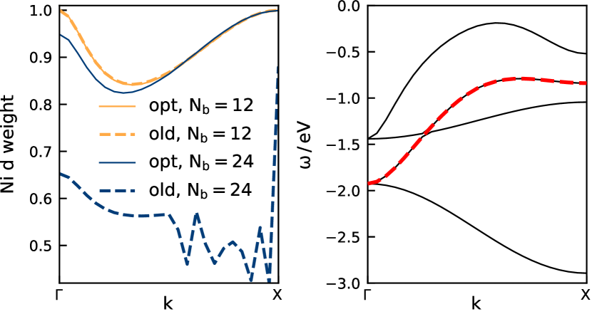
In figure 1 we analyze the orbital properties of selected eigenstates of the resulting Hamiltonian. The left panel shows the Ni $d$ weight of a single band (displayed as red dashed line in the right panel) across a k-path from the $\Gamma$ to the $X$ point. For a small number of unoccupied bands, (total number of bands $N_{b}=12$), the non-optimized and optimized projectors give nearly identical results. However, by including additional unoccupied bands ($N_{b}=24$) the two schemes display huge differences. While the optimized projectors lead to only minor differences to the case of $N_{b}=12$ close to the $\Gamma$ point, the non-optimized projectors lead to considerably less overall Ni $d$ weight and a strongly discontinuous behavior for part of the $k$ pathway. This underlines the advantage of the optimized projectors.

The erroneous behavior of the non-optimized projectors roots in additional high energy bands having Ni-$4d$ character. Using the standard VASP “projectors”, these high lying valence orbitals show appreciable overlap with the $4d$ partial waves (and $4d$ projectors). VASP used to lump the $4d$ and $3d$ contributions into single values, which causes the issues we have just observed. Without going into mathematical details one can easily understand this behavior. The $3d$ or $4d$ states are automatically orthogonal, because the $4d$ states possess an additional node inside the PAW sphere. By simply adding up the contributions from the $3d$ and $4d$ projectors pretending that they correspond to a single main quantum number, and then performing an orthogonalization, the total charge in each $d$ spin channel is one instead of two, explaining the large reduction of the $d$ character using the old scheme.

The failure of the unoptimized projectors could in principle be avoided by simply not including additional empty bands in the construction of the Wannier functions. However, there are important cases where this is not possible. First of all, the situation of $4d$ states close to the Fermi energy is realized in many late transition metals. Second, one might be interested in quantities that include transitions to unoccupied states over large energy scales, such as optical spectroscopy. In these cases, the optimized projectors give reliable results. Furthermore, from a physical point of view, the projectors should not depend strongly on the inclusion of unoccupied states.

3.2 Hartree-Fock Approximation

The DFT+U approach improves the LDA and GGA description of NiO by supplementing the Ni $d$ states by local Coulomb interaction which leads to a static local self energy in (25).

There are two ways to formulate DFT+U: First, the traditional one, where the Kohn-Sham potential is directly augmented with a potential arising from the Hartree-Fock decoupling of the local Hubbard interaction. Second, in terms of a charge self-consistent DFT+DMFT scheme, where the DMFT impurity problem is solved in the Hartree-Fock approximation called DFT+DMFT(HF) in the following. Both schemes are fully equivalent if the augmentation spaces are chosen to be strictly the same and the way spin-polarization is accounted for is the same.

However, many DFT+U implementations, including the one in vasp, work with angular-momentum-decomposed charge densities, which in general do not relate to proper projectors in the definitions of the ”+U” potentials.[32] Additionally, DFT+DMFT and DFT+U for magnetic materials can work with or without spin polarization in the DFT part.

In the following, we compare DFT+U as implemented in vasp to DFT+DMFT(HF) with and without charge self-consistency for the testbed material NiO, and investigate the dependence of the electronic spectra on the double-counting.

Figure 2: Partial density of states for spin up of Ni $d$ and O $p$ states from a) charge self-consistent DFT+DMFT(HF) with $\mu^{\textsc{dc}}=62.5\ \mathrm{eV}$ and b) vasp DFT+U with FLL double counting. Ni₁ and Ni₂ refers to the two different Ni atoms in the unit cell arising due to the anti-ferromagnetic ordering. The spin-up density of the atom Ni₁ is equal to the spin-down density of Ni₂ and vice versa. The oxygen atoms in the unit cell show no spin polarization, thus, O₁ is equivalent to O₂.

We fix the double counting in the vasp DFT+U approach according to a prescription known as “fully localized limit” (FLL)[33] which leads to an orbital independent and diagonal version of $\Sigma_{mm^{\prime}}^{\textsc{dc}}$ in (25), in short $\mu^{\textsc{dc}}$. For a meaningful comparison of spectral features we choose the double counting potential in the DFT+DMFT(HF) approach such that we reproduce the size of the gap in vasp DFT+U, leading to $\mu^{\textsc{dc}}=62.5\ \mathrm{eV}$.

We sample the Brillouin zone of the unit cell of twice the size of the primitive one using $8\times 8\times 8$ k-points and parametrize the Coulomb interaction using Slater integrals given by effective Coulomb parameters $U=8$ eV and $J=1$ eV as obtained from constrained LDA calculations.[28] We perform spin polarized calculations considering antiferromagnetic ordering of the two Ni atoms in the unit cell, where for both, DFT+DMFT(HF) and vasp DFT+U, we only consider spin polarization in the Hartree-Fock part but not in the DFT part.

The respective density of states for spin up are presented in figure 2. In general, the DOS from DFT+U and DFT+DMFT(HF) are very similar: a gap of about $4$ eV is opened between heavily spin-polarized Ni states in the conduction band and strongly hybridized Ni-O states in the valence band. Only details differ for the two approaches, such as a slightly larger spin polarization of Ni states and a larger O contribution at the valence band edge for DFT+DMFT(HF).

Figure 3: Color-coded density of states from DFT+DMFT(HF) for double-counting potentials $\mu^{\textsc{dc}}$ in steps of $0.5$ eV for a) full charge self-consistency and b) one-shot calculations. The respective $\mu^{\textsc{dc}}$ from FLL and AMF are depicted as dashed lines, where AMF in the case of charge self-consistency is $53.5$ eV and therefore out of the plotting range.

The double-counting problem poses a serious problem when using many-body corrections in DFT+DMFT approaches predictively, since fundamental properties such as the single particle gap depend on the double counting. Here, we perform fully charge self-consistent (fcsc) as well as one-shot DFT+DMFT(HF) calculations for various fixed double-counting potentials $\mu^{\textsc{dc}}$ to investigate its influence on the spectra and on the gap.

Strictly speaking, this approach does not represent a proper double-counting scheme on first sight, since there seems to be no functional relation between the double-counting potential $\mu^{\textsc{dc}}$ and energy $E_{\textsc{dc}}$. However, one can motivate this approach following arguments in [34]. Instead of using the standard FLL form for the double-counting correction, one introduces an interaction parameter $U^{\prime}$ in the double counting formulas, which is allowed to be slightly different from $U$ used otherwise in the calculation. In that way, one can again relate $\mu^{\textsc{dc}}$ to a proper energy correction $E_{\textsc{dc}}$.

However, here we are not interested in total energies but in a systematic investigation of the influence of the double counting on the spectral properties. That is why we refrain from an explicit introduction of this parameter $U^{\prime}$. Furthermore, we want to circumvent here further complicating ambiguities in usual double-counting approaches (e.g., if one should use the formal or self-consistent occupation in formulas for $E_{\textsc{dc}}$).[30]

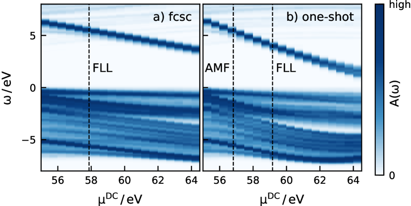
The resulting total DOS for the fcsc and one-shot calculations are presented color coded in figure 3. In both cases the Ni states in the conduction band (dark blue around $5$ eV) are shifted linearly towards the Fermi energy as $\mu^{\textsc{dc}}$ increases. The O/Ni states at the valence band edge are not affected strongly by the double counting. This is because, in general, the higher the Ni character of a band, the more its energy is shifted by the double-counting correction.

In the conduction band we also find states with low spectral weight in the PAW spheres (i.e., they are neither located around the Ni nor the O atoms but in the interstitial region); their energies shift to lower values with decreasing $\mu^{\textsc{dc}}$, i.e., in the opposite direction than the Ni state in the conduction band. For $\mu^{\textsc{dc}}\lesssim 58$ eV in case of fcsc and $\mu^{\textsc{dc}}\lesssim 57$ eV in the case of one-shot calculations, these states cross the Ni states. Then, the conduction band edge does not consist of Ni states, which is not in agreement with experiment. Note that the “around-mean-field” AMF prescription lies in this regime both for one-shot and fcsc calculations and is thus not suitable for NiO. Similarly, the FLL prescription for fcsc calculations is very close to this regime.

For values of the double counting that give the correct conduction band character, the gap shrinks with increasing $\mu^{\textsc{dc}}$. This dependence differs strongly for the one-shot and charge self-consistent calculations: the slope of the gap $dE_{g}/d\mu^{\textsc{dc}}$ in the physical regime differs by a factor of nearly 2. Thus, the charge self-consistency does not cure but alleviates the double-counting problem by decreasing the influence of $\mu^{\textsc{dc}}$ on the spectrum.

4 Benchmark for SrVO₃ monolayer

SrVO₃ presents an example of a correlated transition-metal oxide experiencing a metal-insulator transition (MIT) driven by a dimensional crossover. [35] In particular, a monolayer of SrVO₃ grown on a SrTiO₃ substrate is an insulator with a Mott gap of around 2 eV. In DFT, the compound is found to be metallic and one has to combine DFT with a many-body technique to achieve the correct insulating solution. The related problem of a double layer of SrVO₃ shows insulating behavior in a non charge self-consistent DFT+DMFT treatment. [36]

Here, we use a monolayer of SrVO₃ to benchmark the fully charge-self-consistent (fcsc) DFT+DMFT implementation of triqs/dfttools[23] within the vasp PLO formalism. The motivation for choosing this particular system is that electronic correlations induce an appreciable charge redistribution, making the use of a fcsc DFT+DMFT scheme imperative. Importantly, using the triqs/dfttools framework, we can benchmark the presented vasp interface to the one that is based on the wien2k DFT package,[22] also implemented in triqs/dfttools. Furthermore, we compare our results to previously published fcsc data, also based on the wien2k code, but using MLWF as correlated basis set.[13]

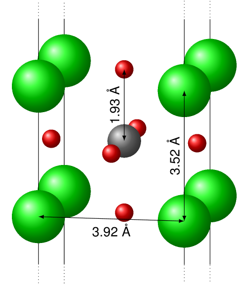
The system is modeled by a free-standing monolayer of SrVO₃ with the in-plane lattice constant equal to that of SrTiO₃ (3.92 Å), simulating thus the epitaxial geometry. The effect of the substrate is neglected. To isolate the individual layers in a periodic unit cell, a vacuum layer of about 16 Å is used in the vasp calculations.

Based on geometry relaxations on the DFT level, in the out-of-plane direction, the V-O distance is reduced from $1.96$ Å to $1.93$ Å and the Sr-Sr distance from $3.92$ Å to $3.52$ Å. The Brillouin zone is sampled using a $15\times 15\times 1$ $\Gamma$-centered Monkhorst-Pack $k$-grid. The energy cutoff of the plane wave basis set is $400$ eV, in accordance with the default value for the PAW potentials used. Using the procedure described above, the projectors onto the V $d$-states are calculated according to (12) by optimizing in an energy window around the Fermi level given by $\varepsilon^{P}_{\min}=-2$ eV and $\varepsilon^{P}_{\max}=1.1$ eV (i.e., states with mainly $t_{2g}$ character) and orthonormalizing according to (14) in the same energy window. In the $t_{2g}$ subspace, a Hubbard-Kanamori interaction with $U=5.5$ eV and $J=0.75$ eV (in agreement with [13]) is added; the resulting double counting is estimated in the FLL scheme.[33, 37] The impurity problem is solved using the triqs/CTHYB Quantum Monte Carlo[38] solver at an inverse temperature $\beta=40\ \mathrm{eV}^{-1}$.

Figure 4: The unit cell of the monolayer of SrVO₃. The Sr atoms are green, the V atom gray and the O atoms red. The lattice constant in the $z$-direction is $20$ Å, i.e., there is about 16 Å of vacuum between the periodic replica of the layers, effectively giving an isolated monolayer.

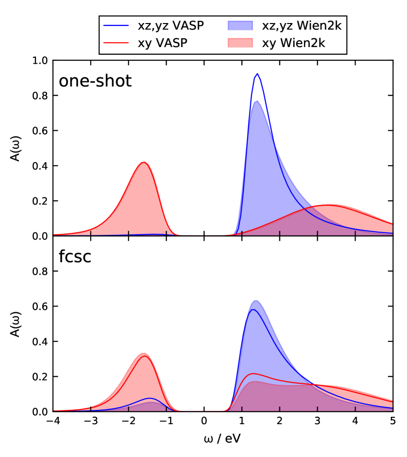
The one-shot DFT+DMFT calculation results in a nearly complete polarization of the orbitals (see fillings in table 1), which is found to be equal in vasp and wien2k, and which is also in accordance with published data.[13] When using the charge feedback in the fcsc framework, the empty orbitals become partly repopulated. This effect happens slightly stronger in vasp but the agreement of the two calculations based on the two different DFT codes is within the expected difference between the two implementations. This re-population can also be seen in the spectral function (figure 5), which is obtained using analytic continuation of the local lattice Green’s function using the maximum entropy method.[39] Unlike the one-shot calculation (top panel of figure 5), the fcsc scheme produces a lower Hubbard band with non-negligible spectral weight also for the degenerate $d_{xz}$ and $d_{yz}$ orbitals (bottom panel of figure 5). The same Mott gap (whose value is in good agreement with experiment [35]) is found starting from both DFT codes, with the peak positions being basically identical. The difference in peak height is compatible with the difference of filling between the two methodologies. The calculated spectra are in excellent agreement with results presented in [13].

Table 1: Filling of the correlated orbitals in DFT+DMFT for one-shot and fully charge self-consistent calculations based on vasp and wien2k.

• 	one-shot		fcsc
  	$d_{xy}$	$d_{xz}$, $d_{yz}$	$d_{xy}$	$d_{xz}$, $d_{yz}$
  vasp	0.96	0.02	0.68	0.16
  wien2k	0.96	0.02	0.76	0.12

Figure 5: DFT+DMFT spectral function of the single layer of SrVO₃ in a one-shot (top) and fully charge self-consistent calculation (bottom). The calculations have been performed using triqs/dfttools, once with wien2k (compare [13]) and once with vasp as underlying DFT code. The resulting imaginary-time Green’s function was analytically continued using the Maximum Entropy Method.[39]

Full charge self-consistency allows us to calculate reliably the total energy as a function of structural parameters and to determine the lowest-energy structure in DFT+DMFT. Here, as a proof of principle, we calculate the total energy of the compound as a function of the distance between Sr-O and V-O planes. We consider deviations $\Delta z$ from the DFT-optimized structure. Positive $\Delta z$ means that the upper Sr-O plane gets shifted upwards and the lower plane gets shifted downwards, thus increasing the thickness of the slab in $z$ direction. This changes the splitting between the $d_{xy}$, which is close to half-filling, and the degenerate $d_{xz}$ and $d_{yz}$ orbitals, which are nearly empty. For more negative $\Delta z$ (i.e., thinner slabs), the $d_{xy}$ orbital approach even more half-filling, while the $d_{xz}$ and $d_{yz}$ orbitals are progressively emptied (see figure 6, bottom). Additionally, the bandwidth decreases, enhancing thus the correlations and the size of the Mott gap (not shown here). The main result of this total-energy calculation is that the minimum calculated with DFT+DMFT is shifted significantly towards lower $\Delta z$ (Figure 6, top), indicating that the structure with the lowest energy has a smaller slab width than obtained by DFT.

Figure 6: Top: Total-energy change of the single layer of SrVO₃ when moving the upper and lower Sr-O-plane symmetrically by $\Delta z$ (from the DFT-optimized structure for $\Delta z=0$) in DFT and in fully charge self-consistent DFT+DMFT. For convenience, the energy for $\Delta z=0$ is shifted to $0$ in each case. Bottom: Filling of the degenerate $d_{xz}$ and $d_{yz}$ orbitals per spin channel as a function of $\Delta z$. The total filling of the impurity is 1 electron. The lines in both plots are guides to the eye. The values and error bars of the DFT+DMFT calculations in both plots were obtained by calculating the quantity for the four last iterations and then determining the mean and the standard deviation. For many data points the error bars are smaller than the markers. The total energy in DFT was converged to $10^{-6}$ eV.

The trend in the structural change can be roughly explained in terms of an additional energy gain by removing the degeneracy between the in-plane $d_{xy}$ and out-of-plane $d_{xz}$, $d_{yz}$ orbitals for smaller values of $\Delta z$. Indeed, having both types of orbitals occupied results in an additional energy cost proportional to interorbital coupling $U-3J$. Once the apical oxygen is moved sufficiently close to the V ion, the anti-bonding orbitals $d_{xz}$, $d_{yz}$ are pushed up in energy and only $d_{xy}$ remains occupied (half-filled). This removes the interorbital energy cost, lowering thus the total energy.

5 Conclusion

We have presented a charge self-consistent implementation to combine DFT with many-body techniques in the vasp package, based on optimized projector localized orbitals (PLO) in the PAW framework. The implemented optimization, seeking the partial wave with the largest overlap with the relevant correlated subspace, is crucial for concise projections and leads to a straight-forward connection between delocalized Kohn-Sham states and localized basis functions. As usual, in the localized subspace, Hubbard-like Hamiltonians can be used straightforwardly. In contrast to a maximally-localized Wannier projection, the projector formalism is very simple, easy to implement, preserves symmetry, and does not require any special precautions for strongly entangled bands. Therefore, the projector formalism is also well suited for the simulation of correlation effects in supercells with a large number of bands. We have exemplified the benefits of using optimized projectors for the case of NiO.

We have benchmarked our fcsc implementation for two cases. First, we have compared a standard vasp DFT+U calculation with a charge self-consistent mean-field treatment of the DFT+DMFT Hamiltonian for the case of NiO. We find only small deviations for the DOS, which we relate to different projections used in the standard vasp DFT+U and the DFT+DMFT scheme. For NiO an important finding is that the double-counting problem is alleviated by the charge self-consistency. With charge self-consistency the influence of the double-counting parameter on the band gap is reduced by about a factor 2 compared to one-shot calculations.

Second, we simulated a SrVO₃ monolayer and found strong orbital polarization, which is decreased in charge self-consistency. This agrees with previously published results using FLAPW+DMFT. Additionally, as a proof of concept, we calculated the total energies from DFT+DMFT and found that correlation effects lead to structural changes in SrVO₃ monolayers, reducing the apical oxygen height in the single layer.

The presented projector and fcsc scheme can be used to interface basically any many-body method with the vasp package. It offers a robust and concise interface for materials studies as well as future developments of tools for strongly-correlated electron systems.

References

- [1] Ceperley D M and Alder B J 1980 Phys. Rev. Lett. 45(7) 566–569 URL https://link.aps.org/doi/10.1103/PhysRevLett.45.566
- [2] Perdew J P, Burke K and Ernzerhof M 1996 Phys. Rev. Lett. 77(18) 3865–3868
- [3] Görling A 1996 Phys. Rev. A 54(5) 3912–3915 URL https://link.aps.org/doi/10.1103/PhysRevA.54.3912
- [4] Georges A, Kotliar G, Krauth W and Rozenberg M J 1996 Rev. Mod. Phys. 68(1) 13–125
- [5] Lichtenstein A I and Katsnelson M I 1998 Phys. Rev. B 57 6884–6895 URL http://link.aps.org/doi/10.1103/PhysRevB.57.6884
- [6] Kotliar G, Savrasov S Y, Haule K, Oudovenko V S, Parcollet O and Marianetti C A 2006 Reviews of Modern Physics 78 865–951 ISSN 0034-6861
- [7] Blöchl P E 1994 Phys. Rev. B 50(24) 17953–17979
- [8] Amadon B, Lechermann F, Georges A, Jollet F, Wehling T O and Lichtenstein A I 2008 Phys. Rev. B 77 205112 ISSN 1098-0121
- [9] Karolak M, Wehling T O, Lechermann F and Lichtenstein A I 2011 Journal of Physics: Condensed Matter 23 085601 ISSN 0953-8984 URL http://iopscience.iop.org/0953-8984/23/8/085601
- [10] Pourovskii L V, Amadon B, Biermann S and Georges A 2007 Physical Review B 76 235101
- [11] Haule K, Yee C H and Kim K 2010 Phys. Rev. B 81 195107
- [12] Aichhorn M, Pourovskii L and Georges A 2011 Phys. Rev. B 84(5) 054529 URL http://link.aps.org/doi/10.1103/PhysRevB.84.054529
- [13] Bhandary S, Assmann E, Aichhorn M and Held K 2016 Phys. Rev. B 94 155131
- [14] Grånäs O, Marco I D, Thunström P, Nordström L, Eriksson O, Björkman T and Wills J 2012 Comp. Mat. Sci. 55 295 – 302 ISSN 0927-0256 URL http://www.sciencedirect.com/science/article/pii/S092702561100646X
- [15] Grieger D, Piefke C, Peil O E and Lechermann F 2012 Physical Review B 86 155121 URL https://link.aps.org/doi/10.1103/PhysRevB.86.155121
- [16] Amadon B 2012 J. Phys. C 24 075604
- [17] Gonze X, Jollet F, Abreu Araujo F, Adams D, Amadon B, Applencourt T, Audouze C, Beuken J M, Bieder J, Bokhanchuk A, Bousquet E, Bruneval F, Caliste D, Côté M, Dahm F, Da Pieve F, Delaveau M, Di Gennaro M, Dorado B, Espejo C, Geneste G, Genovese L, Gerossier A, Giantomassi M, Gillet Y, Hamann D R, He L, Jomard G, Laflamme Janssen J, Le Roux S, Levitt A, Lherbier A, Liu F, Lukačević I, Martin A, Martins C, Oliveira M J T, Poncé S, Pouillon Y, Rangel T, Rignanese G M, Romero A H, Rousseau B, Rubel O, Shukri A A, Stankovski M, Torrent M, Van Setten M J, Van Troeye B, Verstraete M J, Waroquiers D, Wiktor J, Xu B, Zhou A and Zwanziger J W 2016 Computer Physics Communications 205 106–131 ISSN 0010-4655 URL http://www.sciencedirect.com/science/article/pii/S0010465516300923
- [18] Kresse G and Joubert D 1999 Phys. Rev. B 59(3) 1758–1775
- [19] Kresse G and Hafner J 1993 Phys. Rev. B 47(1) 558–561
- [20] Kresse G and Furthmüller J 1996 Phys. Rev. B 54(16) 11169–11186
- [21] Parcollet O, Ferrero M, Ayral T, Hafermann H, Krivenko I, Messio L and Seth P 2015 Computer Physics Communications 196 398–415 ISSN 00104655
- [22] Blaha P, Schwarz K, Madsen G, Kvasnicka D and Luitz J 2001 WIEN2k, An augmented Plane Wave + Local Orbitals Program for Calculating Crystal Properties (Techn. Universitaet Wien, Austria, ISBN 3-9501031-1-2.)
- [23] Aichhorn M, Pourovskii L, Seth P, Vildosola V, Zingl M, Peil O E, Deng X, Mravlje J, Kraberger G J, Martins C, Ferrero M and Parcollet O 2016 Computer Physics Communications 204 200–208 ISSN 00104655
- [24] Marzari N, Mostofi A A, Yates J R, Souza I and Vanderbilt D 2012 Rev. Mod. Phys. 84(4) 1419–1475
- [25] Savrasov S Y and Kotliar G 2004 Physical Review B 69 245101
- [26] Sawatzky G A and Allen J W 1984 Physical Review Letters 53 2339–2342 URL https://link.aps.org/doi/10.1103/PhysRevLett.53.2339
- [27] Bengone O, Alouani M, Blöchl P and Hugel J 2000 Physical Review B 62 16392–16401 URL https://link.aps.org/doi/10.1103/PhysRevB.62.16392
- [28] Anisimov V I, Zaanen J and Andersen O K 1991 Physical Review B 44 943–954 URL https://link.aps.org/doi/10.1103/PhysRevB.44.943
- [29] Ren X, Leonov I, Keller G, Kollar M, Nekrasov I and Vollhardt D 2006 Phys. Rev. B 74(19) 195114 URL https://link.aps.org/doi/10.1103/PhysRevB.74.195114
- [30] Karolak M, Ulm G, Wehling T, Mazurenko V, Poteryaev A and Lichtenstein A 2010 Journal of Electron Spectroscopy and Related Phenomena 181 11 – 15 ISSN 0368-2048 proceedings of International Workshop on Strong Correlations and Angle-Resolved Photoemission Spectroscopy 2009 URL http://www.sciencedirect.com/science/article/pii/S0368204810001222
- [31] Leonov I, Pourovskii L, Georges A and Abrikosov I A 2016 Phys. Rev. B 94(15) 155135 URL https://link.aps.org/doi/10.1103/PhysRevB.94.155135
- [32] Amadon B 2012 Journal of Physics: Condensed Matter 24 075604 ISSN 0953-8984 URL http://stacks.iop.org/0953-8984/24/i=7/a=075604
- [33] Anisimov V I, Solovyev I V, Korotin M A, Czyżyk M T and Sawatzky G A 1993 Physical Review B 48 16929–16934 URL http://link.aps.org/doi/10.1103/PhysRevB.48.16929
- [34] Park H, Millis A J and Marianetti C A 2014 Phys. Rev. B 89(24) 245133 URL https://link.aps.org/doi/10.1103/PhysRevB.89.245133
- [35] Yoshimatsu K, Okabe T, Kumigashira H, Okamoto S, Aizaki S, Fujimori A and Oshima M 2010 Phys. Rev. Lett. 104(14) 147601 URL https://link.aps.org/doi/10.1103/PhysRevLett.104.147601
- [36] Zhong Z, Wallerberger M, Tomczak J M, Taranto C, Parragh N, Toschi A, Sangiovanni G and Held K 2015 Physical Review Letters 114 246401 URL https://link.aps.org/doi/10.1103/PhysRevLett.114.246401
- [37] Held K 2007 Adv. Phys. 56 829–926
- [38] Seth P, Krivenko I, Ferrero M and Parcollet O 2016 Computer Physics Communications 200 274–284 ISSN 00104655
- [39] Bryan R K 1990 Solving oversampled data problems by Maximum Entropy (Dordrecht: Kluwer Academic Publishers) pp 221–232 ISBN 978-94-009-0683-9