Impact Excitation of a Seismic Pulse and Vibrational Normal Modes on Asteroid Bennu and Associated Slumping of Regolith

Abstract

We consider an impact on an asteroid that is energetic enough to cause resurfacing by seismic reverberation and just below the catastrophic disruption threshold, assuming that seismic waves are not rapidly attenuated. In asteroids with diameter less than 1 km we identify a regime where rare energetic impactors can excite seismic waves with frequencies near those of the asteroid’s slowest normal modes. In this regime, the distribution of seismic reverberation is not evenly distributed across the body surface. With mass-spring model elastic simulations, we model impact excitation of seismic waves with a force pulse exerted on the surface and using three different asteroid shape models. The simulations exhibit antipodal focusing and normal mode excitation. If the impulse excited vibrational energy is long lasting, vibrations are highest at impact point, its antipode and at high surface elevations such as an equatorial ridge. A near equatorial impact launches a seismic impulse on a non-spherical body that can be focused on two additional points on an the equatorial ridge. We explore simple flow models for the morphology of vibration induced surface slumping. We find that the initial seismic pulse is unlikely to cause large shape changes. Long lasting seismic reverberation on Bennu caused by a near equatorial impact could have raised the height of its equatorial ridge by a few meters and raised two peaks on it, one near impact site and the other near its antipode.

1 Introduction

Impact induced seismic waves and associated seismic shaking can modify the surface of an asteroid. Impact induced seismicity is a surface modification process that is particularly important on small asteroids due to their low surface gravity and small volume which limits vibrational energy dispersal (Cintala et al., 1978; Cheng et al., 2002; Richardson et al., 2004). Seismic disturbances can destabilize loose material resting on slopes, causing downhill flows (Titley, 1966; Lambe and Whitman, 1979), crater degradation and crater erasure (Richardson et al., 2004; Thomas and Robinson, 2005; Richardson et al., 2005; Asphaug, 2008; Yamada et al., 2016) and particle size segregation or sorting (Miyamoto et al., 2017; Matsumura et al., 2014; Tancredi et al., 2015; Pereraa et al., 2016; Maurel et al., 2017). Flat deposits at the bottom of craters on Eros known as “ponds” can be explained with a seismic agitation model (Cheng et al., 2002), though electrostatic dust levitation may also be required to account for their extreme flatness and fine grained composition (Robinson et al., 2001; Colwell et al., 2005; Richardson et al., 2005). Regions of different crater densities on asteroid 433 Eros are explained by large impacts that erase craters (Thomas and Robinson, 2005). Seismic shaking accounts for slides, slumps, and creep processes on the Moon (Titley, 1966) and on Eros (Veverka et al., 2001), particle size segregation or sorting on Itokawa (Miyamoto et al., 2017; Tancredi et al., 2015) and smoothing of initially rough ejecta on Vesta, a process called ‘impact gardening’ (Schröder et al., 2014).

During the contact-and-compression phase of a meteor impact, a hemispherical shock wave propagates away from the impact site (Melosh, 1989). As the shock wave attenuates, it degrades into normal stress (seismic) waves (e.g., Richardson et al. 2004, 2005; Jutzi et al. 2009; Jutzi and Michel 2014). The seismic pulse, sometimes called ‘seismic jolt’ (Nolan et al., 1992) or ‘global jolt’ (Greenberg et al., 1994, 1996), travels as a pressure wave through the body. Seismic agitation is most severe nearest the impact site and along the shortest radial paths through the body because of radial divergence and attenuation of the seismic pulse (Thomas and Robinson, 2005; Asphaug, 2008). After the seismic energy has dispersed through the asteroid, continued seismic shaking or reverberation of the entire asteroid may continue to modify the surface (Richardson et al., 2005). Small impacts could excite seismic waves that overlap in time as they attenuate, causing continuous seismic noise known as ‘seismic hum’ (Lognonné et al., 2009). The regime that is important for a particular impact and surface modification process depends on the frequency spectrum of seismic waves launched by the impact and the frequency dependent attenuation, scattering and wave speed of the seismic waves (Richardson et al., 2005; Michel et al., 2009).

The size of an impactor that catastrophically disrupts an asteroid exceeds by a few orders of magnitude the size of one that causes sufficient seismic shaking to erase craters (Richardson et al., 2005; Asphaug, 2008). In a rarer event, an asteroid could be hit by a projectile smaller than the disruption threshold but large enough to significantly shake the body. It is this regime that we consider here. We explore the nature of shape changes caused by vibrational oscillations excited by a subcatastrophic impact. With the imminent arrival in 2018 of the OSIRIS-REx mission at Bennu (Asteroid 101955), we investigate the possibility that the unusual shape of Bennu’s equatorial ridge is due to a energetic but subcatastrophic impact.

Asteroids are often modeled as either fractured monoliths or rubble piles. In dry granular media on Earth, pressure waves propagate through particles and from particle to particle through a network of contact points, called ‘force chains’ (Cundall and Strack, 1979; Ouaguenouni and Roux, 1997; Geng et al., 2001; Clark et al., 2012). Laboratory experiments find that the elastic wave speed tends to scale with the classic speed $\sqrt{E/\rho}$ where $E$ is the Young’s modulus and $\rho$ is the density, and is not usually dependent on the particle size, but is weakly dependent on the constraining pressure and porosity (Duffy and Mindlin, 1957). Thus a continuum elastic material model can approximate the seismic behavior of granular materials and has been used to model seismicity in asteroids (e.g., Murdoch et al. 2017). However, if the force chains are dependent on gravitational acceleration, terrestrial and lunar granular materials may not provide good analogs for asteroids which have low surface gravity. Rubble pile asteroids may have a small, but finite, level of tensile strength (Richardson et al., 2009) due to van der Waals forces between fine particulate material (Sánchez and Scheeres, 2014; Scheeres and Sánchez, 2018), so both compressive and tensile restoration forces may be present allowing seismic waves to reflect. Even without cohesion, contacts under pressure allow seismic waves to propagate (e.g., Sánchez and Scheeres 2011; Tancredi et al. 2012). Ballistic contacts also allow a pressure pulse to propagate, as illustrated by the classic toy known as Newton’s cradle.

Unfortunately, little is currently known about how seismic waves are dispersed, attenuated and scattered in asteroids. The rapidly attenuated seismic pulse or jolt model (Thomas and Robinson, 2005) is consistent with strong attenuation in laboratory granular materials at kHz frequencies (O’Donovan et al., 2016), but qualitatively differs from the slowly attenuating seismic reverberation model (Cintala et al., 1978; Cheng et al., 2002; Richardson et al., 2004, 2005), that is supported by measurements of slow seismic attenuation in lunar regolith (Dainty et al., 1974; Toksöz et al., 1974; Nakamura, 1976). While both seismic jolt and reverberation processes can cause crater erasure and rim degradation, size segregation induced by the Brazil nut effect relies on reverberation (e.g., Miyamoto et al. 2017; Tancredi et al. 2012; Matsumura et al. 2014; Tancredi et al. 2015; Pereraa et al. 2016; Maurel et al. 2017).

Despite the poorly constrained seismic wave transport behavior in asteroids, a linear elastic material simulation model may describe the propagation of impact generated seismic waves (e.g., Murdoch et al. 2017). To model the propagation of seismic waves, we use the mass-spring and N-body elastic body model we have developed to study tidal and spin evolution of viscoelastic bodies (Quillen et al., 2016a; Frouard et al., 2016; Quillen et al., 2016b, 2017). As shown by Kot et al. (2015), in the limit of large numbers of randomly distributed mass nodes and an interconnected spring network comprised of at least 15 springs per node, the mass spring model approximates an isotropic continuum elastic solid. We use our mass-spring model to examine the surface distribution of vibrational energy excited by an impact. In this respect we go beyond previous works which have primarily focused on simulation of rubble piles (e.g., Walsh et al. 2012; Holsapple 2013; Schwartz et al. 2013, 2014; Pereraa et al. 2016) and transmission of seismic pulses in planar sheets or spherical bodies (e.g., Tancredi et al. 2012; Murdoch et al. 2017).

In the following section (§2), we summarize properties of Bennu. Normalized units for the problem are discussed in section §2.1 and we estimate frequencies for its vibrational normal modes (section §2.2). In section §3 we discuss excitation of seismic waves by an impact. We identify a regime where low frequency normal modes are likely to be excited by an impact. In section §4 we describe our mass/spring model simulations. We simulate impacts by applying a force pulse to the simulated asteroid surface and the strength and duration of the applied force pulse are estimated from scaling relations described in section §3. Normal modes are identified in the spectrum of the vibrationally excited body. We examine the pattern of vibrational kinetic energy on the surface for three different shape models. In section §5 we explore how impact excited seismic vibrations could induce granular flows on Bennu’s surface. A summary and discussion follows in §6.

Figure 1: The preliminary Bennu shape model by Nolan et al. (2013) is shown in orthographic (perspective) projections. Colors show the geometric height or radius from geometric center. The left two panels show polar views and the right two panels show views with the polar axis on the top. The polar views seen on the upper and lower left panels show that the equatorial ridge has a square-like shape.

Figure 2: Surface geometric height (distance from center) of the Bennu shape model is shown as a function of latitude and longitude. The colorbar is in units of the mean equatorial radius. The longitude extends past $2\pi$ so the right side of the figure repeats the region between 0 and $\pi/2$. We do this so that the equatorial peak near 0 is easier to see. There are four peaks near the equator. Each peak has an antipodal counterpart. The equatorial ridge deviates from the equatorial plane, going above and below $0^{\circ}$ latitude by a few degrees.

2 Bennu

The OSIRIS-REx mission, launched in 2016, (Lauretta et al., 2017) to Bennu (Asteroid 101955), aims to fire a jet of high-purity nitrogen gas onto Bennu’s surface so as to excite at least 60 g of regolith that can be collected and returned to Earth. A C-complex asteroid, Bennu is interesting due to its primitive nature. Spectroscopic measurements are consistent with CM-carbonaceous-chondrite-like material and Bennu’s thermal inertia implies that its surface supports a regolith comprised of sub-cm-sized grains (Emery et al., 2014). A suite of remote sensing observations during 2018 and 2019 will be used to create a series of global maps to characterize the geology, mineralogy, surface processes, and dynamic state of Bennu. These maps will also be used to choose a sample selection site and place the returned sample in geological context. Measurements from the OSIRIS-REx rendezvous will be used to test theories for the formation of Bennu’s equatorial ridge (Scheeres et al., 2016).

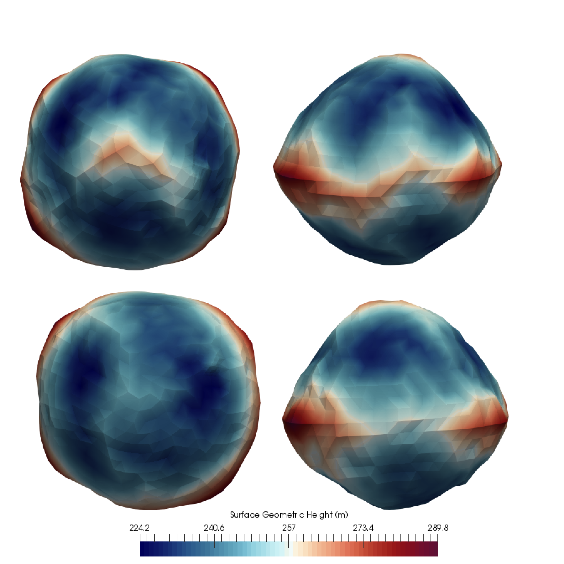
Ground-based radar has been used to characterize Bennu’s shape, spin state, and surface roughness (Nolan et al., 2013). Bennu’s shape is nearly spherical but like 1999 KW4 (Scheeres et al., 2006), Bennu has an equatorial ridge. The shape model consists of 1148 vertices, with a spacing of 25 m between vertices and two subdivided regions with additional resolution where there are protruding features that could be boulders. The shape model was generated by using the vertex locations, estimated Doppler broadening and the radar scattering function, to match the radar images and enforced a uniform mass distribution and principal-axis rotation (Nolan et al., 2013). In Figure 1 and 2 we show the geometric height (distance from geometric center of body). Figure 1 shows 4 orthographic projections. The left two panels show polar views and the right two panels show equatorial views. The polar axis is aligned with the axis of rotation. We use latitude $\lambda$ and longitude $\phi$ angles of the body with respect to the center of mass and spin axis, which we assume is aligned with a principal body axis (following Nolan et al. 2013). The body spin and higher equatorial elevation reduce the radial acceleration on the equatorial ridge. The acceleration is only about 30 $\mu{\rm m/s}^{2}$ on the equatorial ridge, as compared to 85 $\mu{\rm m/s}^{2}$ on the poles (see Figure 11 by Scheeres et al. 2016). Vibrational excitations on the equator are most likely to modify the surface or change the shape of the asteroid.

The individual radar images by Nolan et al. (2013) show that the asteroid shape significantly deviates from a sphere and the body’s equatorial ridge has some smaller scale structure. Individual radar images show significant deviations from a smooth curve that would be consistent with an ellipsoid, so peaks on Bennu’s equatorial ridge could be real and not due to noise in the radar images or uncertainties in the shape model. A polar view shows that Bennu’s equator has a slightly square shape, (see the the left two plots in figure 1). The shape model exhibits four equatorial peaks, and each peak has an antipodal counterpart on the opposite side of the equatorial ridge. The peak longitudes are approximately 20^∘, 110^∘, 190^∘ and 290^∘. The four peaks are not exactly separated by $90^{\circ}$ and the equatorial ridge is not exactly equatorial as it deviates by a few degrees in latitude above and below the equatorial plane. Unfortunately the ground-based shape model may not be sufficiently constrained or unique to know whether Bennu’s equatorial ridge is geometrically suggestive of a periodic process, like Pan’s sculpted ravioli-shaped equatorial ridge. With the imminent arrival of OSIRIS-REx at Bennu, early Dec. 2018, we should soon have a high resolution imaging of Bennu to improve upon this shape model.

We summarize theories of Bennu’s shape evolution following Scheeres et al. (2016). The equatorial ridge may have formed through landslides of surface regolith flowing down to the equatorial region which, because of body spin, is a geopotential low (Guibout and Scheeres, 2003; Scheeres et al., 2006; Walsh et al., 2008, 2012; Hirabayashi et al., 2015). Another mechanism for formation of the equatorial ridge involves infall of material that was fissioned off the parent body due to a binary asteroid interaction (Jacobson and Scheeres, 2011). Alternatively, the interior could undergo a plastic deformation that propagates outwards along the equatorial plane of the body (Hirabayashi and Scheeres, 2015). None of these theories propose an explanation for a possible four pointed structure on the equatorial ridge. This motivates us to explore impact associated shape changes.

Table 1: Physical Quantities for Asteroid Bennu

		physical	N-body
Asteroid Mass	$M$	$7.8\times 10^{10}$ kg	1
Mean equatorial radius	$R_{eq}$	246 m	$\approx 1$
Radius of equivalent volume sphere	$R_{\rm vol}$	$\approx R_{eq}$	1
Average Density	$\rho$	1260 kg m-3	${3}/{(4\pi)}$
Spin Rotation period	$P_{\rm rot}$	4.2978 hours	9.18 $t_{\rm grav}$
Gravitational timescale	$t_{\rm grav}$	1685 s	1
Spin angular rotation rate	$\Omega=2\pi/P_{\rm rot}$	$4.06\times 10^{-4}$ s-1	0.68 $t_{\rm grav}^{-1}$
Energy density	$e_{\rm grav}$	110 Pa	1
Young’s modulus	$E$	11.3 MPa	$10^{5}e_{\rm grav}$
Gravitational speed	$V_{\rm grav}$	0.146 m s-1	1
P-wave speed	$V_{p}$	104 m s-1	712 $V_{\rm grav}$
Characteristic frequency	$f_{\rm char}=V_{p}/R_{\rm vol}$	0.4 Hz	712 $t_{\rm grav}^{-1}$
Notes: The third column gives quantities in physical units. The fourth column gives quantities in N-body or gravitational units. The mass, mean equatorial radius and density, and spin rotation period are those by Chesley et al. (2014). The energy density $e_{\rm grav}$ is computed via equation 3 using the asteroid mass and mean equatorial radius. The gravitational timescale $t_{\rm grav}$ is computed with equation 1. The gravitational velocity $V_{\rm grav}$ is computed with equation 4. The characteristic frequency $f_{\rm char}=V_{p}/R_{\rm vol}$. The P-wave speed is that by Cooper et al. (1974) for lunar surface regolith and the Young’s modulus is estimated from this, the estimated density of Bennu and for a Poisson ratio $\nu=1/4$.

2.1 Sizes, Units and Coordinates

Measurement of the Yarkovsky force gave an estimate for Bennu’s bulk density of $1260\pm 70$ kg/m³, which yields a $GM$ value of $5.2\pm 0.6$ m³/s² (Chesley et al. 2014, total mass $M\approx 7.8\times 10^{10}$ kg). Here $G$ is the gravitational constant. Due to its low density and high porosity ($\sim 40\%$), Bennu is likely to be a rubble-pile (Chesley et al., 2014). The ground-based radar observations used to derive the shape model, also characterize its spin state and surface roughness (Nolan et al., 2013). These observations gave a precise measurement of its rotational period (4.2978 hours). Non-principal-axis rotation has not been detected. The escape speed from Bennu is likely under 23 cm/s and lower than this value at lower latitudes due to spin and body shape (Scheeres et al., 2016). Its mean equatorial radius is estimated at $246\pm 10$ m (Scheeres et al., 2016) and the radius of the equivalent volume sphere, $R_{\rm vol}$, (also called the volumetric radius) is approximately the same value. We list Bennu’s properties (as compiled and measured by Nolan et al. 2013; Chesley et al. 2014) in Table 1. The sizes and units are summarized in both physical and N-body or gravitational units.

For our mass-spring simulations it is convenient to work in units of a gravitational timescale

$$t_{\rm grav} \equiv\sqrt{\frac{R_{\rm vol}^{3}}{GM}}=\sqrt{\frac{3}{4\pi G\rho}}$$

$$=1685{\rm s}\left(\frac{\rho}{1260\ {\rm kg\ m}^{3}}\right)^{\frac{1}{2}}.$$ (1)

The inverse of this timescale is the angular rotation rate of an orbit that just barely grazes the surface of the volume equivalent sphere. The angular rotation rate corresponding to Bennu’s spin rotation period is

$$\Omega=0.68t_{\rm grav}^{-1}\left(\frac{P_{\rm rot}}{4.2978\ {\rm hours}}\right)^{-1}.$$ (2)

A convenient unit of energy density

$$e_{\rm grav}=\frac{GM^{2}}{R_{\rm vol}^{4}}=110\ {\rm kPa}\left(\frac{M}{7.8\times 10^{10}{\rm kg}}\right)^{2}\left(\frac{R_{\rm vol}}{246\ {\rm m}}\right)^{-4}.$$ (3)

Our mass-spring model viscoelastic code typically runs in units of the body mass, $M$, and the radius of the equivalent volume sphere, $R_{\rm vol}$. For Bennu the mean equatorial radius is approximately equal to the radius of the equivalent volume sphere. In these units the mean asteroid density $\rho=3/(4\pi)$. The code unit of velocity is

$$V_{\rm grav}=\sqrt{\frac{GM}{R_{\rm vol}}}=\frac{R_{\rm vol}}{t_{\rm grav}}.$$ (4)

The unit of force $F_{\rm grav}=GM^{2}/R_{\rm vol}^{2}$. Other units can be constructed similarly.

For an isotropic material the P-wave, S-wave and Rayleigh wave velocities are related to the Young’s modulus $E$, mass density $\rho$, and Poisson ratio $\nu$ by

$$V_{p} =\sqrt{\frac{E}{\rho}}\sqrt{\frac{(1-\nu)}{(1+\nu)(1-2\nu)}},$$

$$V_{s} =\sqrt{\frac{E}{\rho}}\frac{1}{\sqrt{2(1+\nu)}},$$

$$V_{Ra} \approx V_{s}\frac{0.862+1.14\nu}{1+\nu}.$$ (5)

where the last relation is approximate (Freund 1998; page 83). We estimate wave speeds using a Poisson ratio of $\nu=1/4$ because our mass spring model approximates a continuum elastic solid with this value (Kot et al., 2015). With Poisson ratio $\nu=1/4$ the P-wave speed and ratios between S-wave and Rayleigh wave speeds are

$$V_{p} =\sqrt{\frac{E}{\rho}}\sqrt{\frac{6}{5}}\approx 1.09\sqrt{\frac{E}{\rho}},$$

$$\frac{V_{p}}{V_{s}} \approx 1.73,$$

$$\frac{V_{Ra}}{V_{s}} \approx 0.92,$$

$$\frac{V_{Ra}}{V_{p}} \sim 0.53.$$ (6)

For a homogeneous body, it takes a time $t=R_{\rm vol}/V_{p}$ for a P-wave to travel from surface to core. The lowest frequency vibrational normal modes are proportional to the inverse of this travel time or a characteristic frequency $f_{\rm char}\equiv V_{p}/R_{\rm vol}$.

Surface layers of the moon have a low P-wave velocity of about $V_{p}\approx 104$ m/s (Cooper et al., 1974) suggestive of a fractured and porous material and consistent with lunar regolith. Taking a Poisson ratio of $\nu=1/4$ and the estimated density of Bennu, the P-wave lunar regolith velocity corresponds to a Young’s modulus of $E=11.3$ MPa. We will adopt this Young’s modulus and this P-wave speed to explore propagation of the impact excited seismic waves in our model, as did Murdoch et al. (2017) to study seismicity on Didymoon (provisionally designated S/2003 (65803) 1).

We use a right handed Cartesian coordinate system in the body frame ${\bf r}=(x,y,z)$ and an associated spherical coordinate system with radius, and latitude and longitude angles $(r,\lambda,\phi)$. The two are related by $(x,y,z)=r(\cos\lambda\cos\phi,\cos\lambda\sin\phi,\sin\lambda)$. We take the z-axis, $\hat{\bf z}$ along the body’s maximum moment of inertia, assuming that this axis is the spin axis and with North pole at positive $z$. Rotation is defined with the surface moving toward the East (increasing $\phi$) as seen from an inertial frame. When using the preliminary Bennu shape model (Nolan et al., 2013), we define latitude and longitude with respect to the coordinates used by the shape model. These angles are not part of any cartographic standard.

2.2 Frequencies of the slowest normal modes for a homogeneous sphere

Is it possible to excite normal modes in a granular system? Laboratory studies of pressure waves and pulses in granular media show weaker attenuation at lower frequencies (e.g., O’Donovan et al. 2016), so the lowest frequency waves should be the last to decay. Laboratory studies find that pulse propagation co-exists with long lived slower, multiply scattered coda-like signals Jia (2004); Jia et al. (1999); Hostler (2005). Lower frequency normal mode oscillations are seen in laboratory experiments of granular media (O’Donovan et al., 2016), though these are typically at about 1 kHz, corresponding to the lowest frequency modes of a box containing granular media in a lab, rather than the Hz scale relevant for Bennu’s normal modes (estimated below). Due to the lower attenuation at low frequencies, normal mode oscillations may be sustainable in an asteroid.

The first in-depth study of an elastic homogeneous sphere is that by Lamb (1881). Modes are separated into spheroidal $S$ and toroidal $T$ types with each mode characterized by the number of surface nodal lines $l$, internal (or radial) nodal lines $n$ and azimuthal order $m$ (e.g., Snieder and Wijk 2015). We ignore torsional modes because they do not give radial displacements, so they would not be strongly excited by impacts or tidal perturbations. For the non-rotating homogeneous sphere, the mode frequencies are independent of $m$. In a spinning body, the normal modes are split and the frequencies depend on $m$ (Montagner and Roult, 2008). However, as the spin rate of Bennu is small (1000 times smaller than the characteristic frequency $f_{\rm char}=V_{p}/R$), the frequency splitting in Bennu and other nearly spherical asteroids should be small. Following Hitchman et al. (2016.), we use notation ${}_{n}f_{l}$ for the spherical (S) normal mode frequencies. With $n=0$ (no radial nodes) the frequencies

$${}_{0}f_{l}=\frac{\sqrt{l(l+1)}}{2\pi}\frac{V_{Ra}}{R}\qquad{\rm for}\qquad l>0$$ (7)

(equation 5 by Hitchman et al. 2016.) where $V_{Ra}$ is the Rayleigh wave velocity. Spherical modes with $n=0$ can be described as constructively interfering Rayleigh waves propagating across the surface.

Evaluating the frequencies of the $n=0$ modes (using equation 7) and using $\frac{V_{Ra}}{V_{p}}=0.53$ for Poisson ratio $\nu=1/4$ (as discussed in section 2.1) we compute for $l=1$ to 5,

$${}_{0}f_{1} =0.119f_{\rm char},$$

$${}_{0}f_{2} =0.207f_{\rm char},$$

$${}_{0}f_{3} =0.292f_{\rm char},$$

$${}_{0}f_{4} =0.377f_{\rm char},$$

$${}_{0}f_{5} =0.462f_{\rm char}.$$ (8)

Spherical modes without surface nodal lines ($l=0$) are often called radial modes and they can be described in terms of interfering P-waves. Again following Hitchman et al. (2016.) the radial modes for a homogeneous sphere are found from the roots of

$$\cot x-\frac{1}{x}+\frac{x}{4}\left(\frac{V_{p}}{V_{s}}\right)^{2}=0.$$ (9)

The radial spherical model frequencies are

$${}_{n}f_{0}=\frac{x}{2\pi}\frac{V_{p}}{R},$$ (10)

where $x$ is a root of equation 9. For a homogeneous sphere and Poisson ratio $\nu=1/4$ giving $\left(\frac{V_{p}}{V_{s}}\right)^{2}=3$ (using equations 5), we find that the first 5 radial frequencies (with $n=0$ to 4) are

$${}_{0}f_{0} =0.41f_{\rm char},$$

$${}_{1}f_{0} =0.96f_{\rm char},$$

$${}_{2}f_{0} =1.48f_{\rm char},$$

$${}_{3}f_{0} =1.98f_{\rm char},$$

$${}_{4}f_{0} =2.49f_{\rm char}.$$ (11)

Figure 3: Scaling for impacts. Diameters of projectiles capable of catastrophic disruption, global seismic shaking and excitation of normal modes. For this plot we use seismic efficiency $\epsilon_{s}=10^{-5}$, seismic amplification $S=1$, P-wave velocity $V_{p}=100$ m/s, impactor velocity $V_{\rm proj}$ = 5 km/s, and density for impactor and asteroid of 2.0 g/cc. The top pink line shows the diameter in km of a projectile capable of catastrophically disrupting a parent body, with diameter shown on the x-axis in km. The disruption threshold is that by Jutzi et al. (2010) for pumice using coefficients from their Table 3 and for a 5 km/s impact. The green triangles and orange dots show projectiles giving a source time equal to the characteristic frequency $f_{\rm char}=R/V_{p}$ and one tenth of this. These are computed with equation 18. With $\tau_{s}\sim R/V_{p}$ we expect excitation of low frequency normal modes. The top axis shows the time for a P-wave to traverse from the surface to the center of the asteroid $R/V_{p}$. Three lower lines (blue, green, black) give minimum impactors capable of causing global seismic shaking (GS) or seismic waves with accelerations greater than the surface gravity. These are computed using equation 9 by Richardson et al. (2005). The accelerations depend on the seismic frequency, $f_{s}$, and we have plotted projectile diameters for peak seismic frequencies $f_{s}=1$, Hz, 10 Hz and 100Hz. The dot-dashed tan line and dashed brown line show global seismic shaking with frequency estimated from the seismic source time (equation 21) and turn over frequency (equation 25). The yellow region shows the regime where a strong impact lies just below catastrophic disruption, but above that giving global seismic reverberation. Impacts in this regime would excite low frequency normal modes.

3 Excitation of Seismic Waves by an Impact

Using scaling arguments (following McGarr et al. 1969; Walker and Huebner 2004; Lognonné et al. 2009), we can describe the excitation of seismic waves from a meteoroid impact in terms of two ratios, one involving the integrated stress of the seismic pulse and the momentum of impactor and the other involving the energy of seismic waves launched by the impact. The seismic impulse $I_{s}$ is the total momentum from the impact transferred into seismic motions,

$$I_{s}\approx\int_{0}^{\tau_{s}}F_{s}(t)dt$$ (12)

where $\tau_{s}$ is the seismic source duration and $F_{s}(t)$ is a time dependent applied force. The contact-and-compression phase of an impact excites a hemispherical shock wave in the ground that propagates away from the impact site (Melosh, 1989). The shock wave attenuates and degrades into an entirely elastic (seismic) wave. The structure of the excited elastic wave is expected to be complex, with multiple pulses associated with the elastic precursor to the shock wave, an elastic remnant to a plastic wave during the transition between shock and elastic wave, and reverberations associated with different seismic impedances in the target, rock fracture and compactification (see section 5.2.6 by Melosh 1989). However, following Lognonné et al. (2009), we can approximate the excitation of the seismic wave with a smooth force function $F_{s}(t)$ applied to the free asteroid surface and in the direction normal to the surface. We neglect a possible horizontal stress component that might arise from a grazing collision.

The seismic amplification $S$ is a dimensionless factor describing the ratio of momentum

$$S\equiv\frac{I_{s}}{m_{\rm proj}V_{\rm proj}},$$ (13)

where $m_{\rm proj}$ is the mass of the projectile and $V_{\rm proj}$ is the projectile speed at the moment of impact relative to the asteroid. The amplification factor for a normal impact has $S\sim 1$, corresponding to a perfectly inelastic impact, however hypervelocity impacts with energetic ejecta can have $S\gtrsim 10$ (McGarr et al., 1969; Holsapple, 2004).

The kinetic energy of the impactor $E_{\rm proj}=\frac{1}{2}m_{\rm proj}V_{\rm proj}^{2}$ and this can be compared to the total radiated seismic energy, $E_{s}$, giving a seismic efficiency factor

$$\epsilon_{s}\equiv\frac{E_{s}}{E_{\rm proj}}.$$ (14)

The seismic efficiency $\epsilon_{s}$ is poorly constrained, and ranges from $\epsilon_{s}\sim 10^{-2}$ to $10^{-6}$ (see experiments and discussions by McGarr et al. 1969; Schultz and Gault 1975; Melosh 1989; Richardson et al. 2005; Shishkin 2007; Lognonné et al. 2009; Yasui et al. 2015; Güldemeister and Wünnemann 2017).

Wolf (1944) derived an expression for the power radiated in seismic waves into a homogeneous elastic half-space by a sinusoidally varying vertical force applied to the surface and that is valid for wavelengths larger than the seismic source. McGarr et al. (1969) used this expression to estimate the seismic radiated power assuming an applied force function in the form

$$F_{s}(t)=F_{s}(1-\cos(2\pi t/\tau_{s}))$$ (15)

that is applied only during $0<t<\tau_{s}$ with $\tau_{s}$, the seismic source duration. Lognonné et al. (2009) (see their equation 5) used the expression by McGarr et al. (1969) to relate the seismic efficiency to the seismic source duration giving

$$\epsilon_{s}\sim 8\pi^{2}0.384\ S^{2}\frac{m_{\rm proj}}{\rho V_{p}^{3}\tau_{s}^{3}},$$ (16)

where $\rho$ is the target asteroid density and $V_{p}$ is the P-wave speed in the target asteroid.

For a homogeneous spherical asteroid of radius $R$ and mass $M=\frac{4}{3}\pi\rho R^{3}$, we can rewrite equation 16 to give

$$\epsilon_{s} \approx 127S^{2}\frac{m_{\rm proj}}{M}\left(\frac{R}{V_{p}\tau_{s}}\right)^{3}.$$ (17)

Using our definition for the characteristic frequency, $f_{\rm char}=V_{p}/R$, and writing the mass ratio $m_{\rm proj}/M$ in terms of a diameter ratio, equation 17 is equivalent to

$$\frac{D_{\rm proj}}{D} \approx 0.2\left(\frac{\rho}{\rho_{\rm proj}}\right)^{\frac{1}{3}}S^{-\frac{2}{3}}\epsilon_{s}^{\frac{1}{3}}\tau_{s}f_{\rm char}$$ (18)

and

$$\tau_{s}f_{\rm char} \approx 5\epsilon_{s}^{-\frac{1}{3}}S^{\frac{2}{3}}\left(\frac{D_{\rm proj}}{D}\right)\left(\frac{\rho_{\rm proj}}{\rho}\right)^{\frac{1}{3}}.$$ (19)

Here $\rho_{\rm proj}$ is the projectile density, and $D$ and $D_{\rm proj}$ are asteroid and projectile diameters.

At a fixed amplification factor $S$ and seismic efficiency $\epsilon_{s}$, equation 19 implies that the seismic source duration times the characteristic frequency is proportional to the ratio of projectile and asteroid diameters. In other words, the projectile diameter sets the seismic source time, with larger projectiles causing longer seismic pulses (see discussion by Güldemeister and Wünnemann 2017). A longer seismic pulse gives a seismic spectrum with more power at lower wave frequencies. Impact simulations show larger projectiles producing a lower frequency spectrum of seismic waves (see Figure 10 by Richardson et al. 2005), and this is consistent with source time increasing with projectile size.

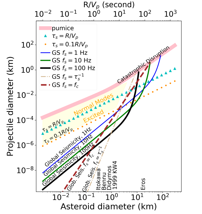
How large a projectile would excite low frequency normal modes? For a homogeneous body, the $n=0$, $l=2$ normal mode has frequency ${}_{0}f_{2}\approx 0.2f_{\rm char}$ (equation 8). A seismic source with source time $\tau_{s}$ should have power at frequency $f\sim 1/\tau_{s}$. So the projectile that gives source time $\tau_{s}f_{\rm char}\sim 1$ should excite low frequency normal modes. Equation 18 applied with $\tau_{s}f_{\rm char}\sim 1$ gives us an estimate for the diameter of a projectile capable of exciting seismic waves at low frequencies, similar to those of the slowest normal modes. To illustrate the regime for excitation of low frequency normal modes by an impact, we plot equation 18 in Figure 3 for $\tau_{s}f_{\rm char}=1$ and 0.1 as turquoise triangles and orange circles, respectively, with $\epsilon_{s}=10^{-5}$, $S=1$ and $\rho_{\rm proj}=\rho$. For Bennu with a diameter $\sim 500$ m, a projectile with diameter 2m (and with impact angle normal to the surface) could produce a seismic source with source timescale that is approximately the inverse of the characteristic frequency and similar in size to the periods of its slowest normal modes.

3.1 Catastrophic disruption and global reverberation thresholds

Equation 18 estimates the size of a projectile that can excite low frequency normal modes. How close is this projectile size to a disruption threshold or a threshold for global seismic reverberation? It is customary to characterize impacts in terms of a specific energy threshold or the kinetic energy in the collision divided by target mass (e.g., Melosh and Ryan 1997; Benz and Asphaug 1999; Jutzi et al. 2010). A catastrophic disruption threshold, $Q_{D}^{*}$, is the specific energy required to disperse the target into a set of individual objects, the largest one having half the mass of the original target. To estimate the disruption threshold, we use equation 3 by Jutzi et al. (2010), coefficients for pumice from their Table 3, a 5 km/s projectile velocity (typical of asteroid encounters; Bottke et al. 1994) and assume that asteroid and projectile have a similar density. In Figure 3 we plot as a wide pink line the projectile diameter corresponding to this disruption threshold as a function of asteroid diameter. An impactor of diameter $D_{\rm proj}\sim 10$m at a projectile velocity of 5 km/s is large enough to catastrophically disrupt Bennu. Figure 3 illustrates that projectiles capable of exciting normal modes in an asteroid are likely to be an order of magnitude smaller than a projectile causing catastrophic disruption.

Assuming a single seismic wave frequency and computing accelerations from the wave, Richardson et al. (2005) estimated the diameter of a projectile $D_{\rm proj}$ sufficient to cause seismic vibration across the whole body that is above the surface gravitational acceleration $g=GM/R^{2}$. The projectile diameter

$$D_{\rm proj}\approx\left[\frac{G^{2}\rho^{3}D^{5}}{9\epsilon_{s}\rho_{\rm proj}V_{\rm proj}^{2}f_{s}^{2}}\right]^{\frac{1}{3}}\exp\left(\frac{2\pi f_{s}D^{2}}{K_{s}\pi^{2}Q3}\right),$$ (20)

(their equation 15 but corrected with a factor of 1/3 in the exponential). Here $f_{s}$ is the frequency of the seismic waves. The seismic attenuation coefficient is $Q$ and $K_{s}$ is a seismic diffusivity. In Figure 3 we have plotted this function for three frequencies $f_{s}=1,10,100$ Hz (as blue, green and black lines) using $\rho=\rho_{\rm proj}=2.0{\rm g/cc}$, seismic efficiency $\epsilon_{s}=10^{-5}$, projectile velocity $V_{\rm proj}=5$ km/s, attenuation coefficient $Q=2000$ and seismic diffusivity $K_{s}=0.1{\rm km}^{2}{\rm s}^{-1}$. We have adopted the $Q$ and $K_{s}$ values used by Richardson et al. (2005). The $Q$ attenuation coefficient is based on $Q=3000$ to 5000 from long period seismic instruments on the Moon (Dainty et al., 1974; Toksöz et al., 1974) and $Q=1600$ to 2300 from short period lunar seismic instruments (Nakamura, 1976). The seismic diffusivity is that estimated from lunar seismic observations (Dainty et al., 1974; Toksöz et al., 1974). As expected, these lines lie below the catastrophic disruption threshold. These lines are also below those we estimated for projectiles capable of exciting normal modes. Projectiles capable of exciting normal modes would cause much larger levels of agitation than those only just capable of crater erasure.

Equation 20 is computed assuming a single seismic frequency dominates the spectrum. Previously we estimated the seismic source time. We can use this timescale to estimate a frequency typical of seismic waves excited by the impact. Taking seismic frequency $f_{s}\sim 1/\tau_{s}$, from the seismic source time, we use equation 18 for $\tau_{s}$ to estimate the frequency of generated seismic waves. Neglecting seismic attenuation, and inserting this frequency into equation 20 gives

$$D_{\rm proj} \sim\frac{0.7G^{2}\rho^{2}S^{\frac{4}{3}}D^{5}}{\epsilon_{s}^{\frac{5}{3}}V_{\rm proj}^{2}V_{p}^{2}}$$ (21)

for the projectile diameter capable of causing global seismic reverberation. This too is plotted in Figure 3 as a dot-dashed tan line using $\rho=\rho_{\rm proj}=2.0{\rm g/cc}$, seismic efficiency $\epsilon_{s}=10^{-5}$, projectile velocity $V_{\rm proj}=5$ km/s, P-wave velocity $V_{p}=100$ m/s, and seismic amplification factor $S=1$. The line is below the constant frequency lines and suggests that smaller impacts can cause significant levels of agitation on smaller asteroids.

3.2 Seismic spectrum corner frequency

We lack a model for the frequency spectrum of seismic waves excited by an impact and up to this point we have estimated the peak frequency using simple source time model, that by Lognonné et al. (2009) and based on estimates by McGarr et al. (1969). However we can also constrain the seismic spectrum radiated by an impact by considering the size of the source region. A seismic source spectrum is limited by the size and duration of the source. If an earthquake source is a delta function in time and the fault area infinitesimally small, then the displacement spectrum is flat (as discussed at the end of section 10.1.4 by Aki and Richards 2002). Here the seismic wave amplitudes are described with material displacements from rest. Otherwise the source spectrum is weaker at frequencies above a particular frequency, that we call the corner frequency. An instantaneous quake cannot efficiently radiate seismic waves with wavelengths smaller than its fault length as the source is coherent in phase. The corner frequency is due to spatial interference (section 10.1.5 by Aki and Richards 2002) and is approximately the wave speed divided by the fault length. Most seismic sources, including those derived from simulations of asteroid impacts, have power spectra dropping at high frequencies (see Figure 10 by Richardson et al. 2005).

Crater diameter has previously been used to estimate a source size for impact radiated seismic waves (Meschede et al., 2011). We can estimate the turn over or corner frequency of the impact radiated seismic spectrum using an estimate for the diameter of the crater formed during impact. Crater sizes on Bennu would be in the strength-scaling regime (Holsapple, 1993) with diameter

$$D_{\rm crater}\sim 30D_{\rm proj}$$ (22)

as approximated in equation 32 by Richardson et al. (2005) (also see their Figure 16 comparing this approximation to the regimes discussed by Holsapple 1993). Housen et al. (2018) has carried out experiments of impacts into porous cohesionless materials. An extrapolation of their highest velocity experiments (by two orders of magnitude past the smallest dimensionless $\pi_{2}$ value on their Figure 15) gives a crater diameter approximately consistent with equation 22.

A corner frequency set from the crater diameter and P-wave velocity

$$f_{\rm corner}\approx\frac{V_{p}}{D_{\rm crater}}\approx\frac{V_{p}}{30D_{\rm proj}}.$$ (23)

The displacement spectrum typically drops at frequencies larger than $f_{\rm corner}$ with a power law form, and is flat at lower frequencies. For an impactor with diameter of 1 m and $V_{p}\sim 100$ m/s, equation 23 gives a corner frequency $f_{\rm corner}\approx 3$ Hz and fairly near the characteristic frequency of Bennu that we estimated at 0.4 Hz in Table 1. In units of the characteristic frequency

$$\frac{f_{\rm corner}}{f_{\rm char}}\sim\frac{D}{60D_{\rm proj}}$$ (24)

so an impactor with diameters about 60 times smaller than that of the asteroid would give a seismic spectrum with corner frequency in the vicinity of the characteristic frequency and so within a decade of the slowest normal modes. This implies that a significant fraction of the seismic wave power for this impact would be emitted at low frequencies and possibly at frequencies similar to those of the slowest normal modes.

Low frequency seismic waves usually take longer to attenuate than high frequency waves, so seismic reverberation caused by a large impact may be long lasting. The energy in an excited normal mode typically lasts an attenuation factor $Q$ times the normal mode period. Another consequence of low frequency content in the seismic waves excited by a strong impact is that seismic reverberation could persist.

Neglecting attenuation and using the corner frequency (equation 24) for the seismic frequency ($f_{s}=f_{\rm corner}$) we can estimate the projectile diameter capable of causing global seismic reverberation again with equation 20, giving

$$D_{\rm proj}=\frac{G\rho D^{3}}{V_{\rm proj}V_{p}}\left(\frac{5}{3\epsilon_{s}}\frac{\rho}{\rho_{\rm proj}}\right)^{\frac{1}{2}}.$$ (25)

This is plotted as a brown dashed line in Figure 3. The line also lies below reverberation thresholds estimated with single seismic frequencies.

3.3 The regime for subcatastrophic impacts that are capable of exciting normal modes

Richardson et al. (2005) estimated a frequency dependent projectile size capable of causing global seismic reverberation at the level of surface acceleration. Using an estimate for the seismic source time and a turn-over or corner frequency for the spectrum based on crater size we modified the estimate so that it was independent of frequency. In both cases the projectile diameter capable of causing global seismic reverberation lies well below the catastrophic disruption threshold for small asteroids and below an estimate for the size of a projectile capable of exciting low frequency seismic waves.

Figure 3 delineates a regime (shown in yellow) where a catastrophic impact can excite vibrational normal modes and with accelerations above surface gravity acceleration. The asteroid is not catastrophically disrupted but the surface accelerations caused by the seismic waves would exceed surface gravity and so launch material off the surface. Material could hop or flow across the surface, but would not necessarily be ejected. When the vibrational spectrum is dominated by a few normal modes, the vibrational energy is not evenly distribution across the surface. The asteroid surface may slump, reaching a final shape that could be sensitive to the morphology of the normal modes themselves.

Figure 3 gives the regime for an asteroid with a slow P-wave velocity consistent with a porous material (such as lunar regolith) and a seismic efficiency of $\epsilon_{s}=10^{-5}$. The catastrophic impact line used here is sensitive to the material of the asteroid. If the asteroid is softer or comprised of solid ice, then the catastrophic impact line is higher on the plot. With a higher seismic efficiency, more energy is excited by the impact and the global seismicity lines are lower on the plot. If the P-wave speed is higher, then we expect the seismic diffusivity $K_{s}$ to be larger. This pushes the attenuation cutoffs for the global seismicity lines to the right on the plot and extends the regime for normal excitation to larger bodies. With a somewhat higher seismic efficiency of $\epsilon_{s}=10^{-4}$ and faster P-wave velocity (3 km/s typical of ice), the larger icy moon Pan (28 km diameter and with a sculpted equatorial ridge), may lie in a regime where a 0.3 km diameter icy impactor could excite normal modes.

Figure 3 shows a regime for a subcatastrophic impact to excite vibrational normal modes. How rare are these impacts on Bennu? The mean time between impacts as a function of impactor diameter has been computed for Mars crossing asteroid 433 Eros by Richardson et al. (2005) based on the asteroid size distribution model by O’Brien and Greenberg (2005). We can estimate the mean time between impactors by multiplying by the ratio of cross sectional areas. The cross sectional area of Bennu is 0.19 km², computed from its mean equatorial radius. The mean time period between 2 m diameter impacts on 433 Eros (with cross sectional area about 360 km²) is about 1000 years, following Figure 16A by Richardson et al. (2005). The ratio of cross sectional areas is 2000 giving a mean time between 2 m diameter impactors on Bennu of 2 million years. Bennu should experience a shape changing encounter about every few million years. The mean time between such impacts is similar to its orbital lifetime as a near-earth object. Such an encounter would not be unlikely, but neither would it happen frequently.

3.4 Force for the seismic pulse

To carry out simulations of an impact, we require a seismic source time and a force amplitude $F_{s}$. Using the definitions for amplification factor $S$ (equation 13) and $I_{s}$ (equation 12 and approximating the integral as $F_{s}\tau_{s}$), and using equation 19 for $\tau_{s}$, the force of the seismic impulse in gravitational units

$$\frac{F_{s}}{GM^{2}/R^{2}} \approx S\left(\frac{\rho_{\rm proj}}{\rho}\right)\left(\frac{D_{\rm proj}}{D}\right)^{3}\left(\frac{V_{\rm proj}V_{p}}{V_{\rm grav}^{2}}\right)\left(\frac{1}{\tau_{s}f_{\rm char}}\right).$$ (26)

We insert equation 18 for the diameter ratio

$$\frac{F_{s}}{GM^{2}/R^{2}} \approx 0.008S^{-1}\epsilon_{s}(\tau_{s}f_{\rm char})^{2}\left(\frac{V_{\rm proj}V_{p}}{V_{\rm grav}^{2}}\right)$$ (27)

$$\approx 2\ S^{-1}\left(\frac{\epsilon_{s}}{10^{-5}}\right)(\tau_{s}f_{\rm char})^{2}$$

$$\times\left(\frac{V_{\rm proj}}{5\ {\rm km~{}s}^{-1}}\right)\left(\frac{V_{p}}{100{\rm\ m~{}s}^{-1}}\right)\left(\frac{V_{\rm grav}}{\ 0.146{\rm\ m~{}s}^{-1}}\right)^{-2}.$$ (28)

In the last line, we have used $V_{\rm grav}$ for Bennu from Table 1. If we replace $\tau_{s}f_{\rm char}$ using equation 19 we find

$$\frac{F_{s}}{GM^{2}/R^{2}} \approx 0.2(\epsilon_{s}S)^{\frac{1}{3}}\left(\frac{D_{\rm proj}}{D}\right)^{2}\left(\frac{\rho_{\rm proj}}{\rho}\right)^{\frac{2}{3}}\left(\frac{V_{\rm proj}V_{p}}{V_{\rm grav}^{2}}\right).$$ (29)

The source time $\tau_{s}f_{\rm char}$ and the force of the impulse $F_{s}$ are not independent, and both are approximately set by the impactor diameter. In section §4 we will use equation 19 for the seismic source time and equation 28 for the impulse force to model an impact generated seismic pulse with our elastic body simulations code.

It may be convenient to estimate the seismic energy of the impact in gravitational units. As we computed $F_{s}$ in gravitational units, the total seismic energy radiated by the impact

$$\frac{E_{s}}{GM^{2}/R} \approx\frac{\epsilon_{s}}{2}\left(\frac{\rho_{\rm proj}}{\rho}\right)\left(\frac{D_{\rm proj}}{D}\right)^{3}\left(\frac{V_{\rm proj}}{V_{\rm grav}}\right)^{2}$$

$$\approx 4\times 10^{-3}S^{-2}\epsilon_{s}^{2}\left(\frac{V_{\rm proj}}{V_{\rm grav}}\right)^{2}(\tau_{s}f_{\rm char})^{3}$$

$$\approx 4\times 10^{-4}S^{-2}\left(\frac{\epsilon_{s}}{10^{-5}}\right)^{2}\left(\frac{V_{\rm proj}}{5{\rm\ km~{}s}^{-1}}\right)^{2}$$

$$\qquad\times\left(\frac{V_{\rm grav}}{\ 0.146{\rm\ m~{}s}^{-1}}\right)^{-2}(\tau_{s}f_{\rm char})^{3}.$$ (30)

4 Elastic Body Simulations

4.1 Mass-spring models

To simulate elastic and vibrational response and transmission of seismic waves we use a mass-spring model (Quillen et al., 2016a; Frouard et al., 2016; Quillen et al., 2016b, 2017) that is built on the modular N-body code rebound (Rein and Liu, 2012). An elastic solid is approximated as a collection of mass nodes that are connected by a network of springs. Springs between mass nodes are damped and so the spring network approximates the behavior of a Kelvin-Voigt viscoelastic solid with Poisson ratio of 1/4 (Kot et al., 2015). When a large number of particles is used to resolve the spinning body the mass-spring model behaves like an isotropic continuum elastic solid (Kot et al., 2015) including its ability to transmit seismic waves.

The mass particles in the resolved spinning body are subjected to three types of forces: the gravitational forces acting between every pair of particles in the body, and the elastic and damping spring forces acting only between sufficiently close particle pairs. Springs have a spring constant $k_{s}$ and a damping rate parameter $\gamma_{s}$. The number density of springs, spring constants and spring lengths set the shear modulus, $\mu$, whereas the spring damping rate, $\gamma_{s}$, allows one to adjust the shear viscosity, $\eta$, and viscoelastic relaxation time, $\tau_{\rm relax}=\eta/\mu$. For a Poisson ratio of 1/4, the Young’s modulus $E=2(1+\nu)\mu=2.5\mu$. The equation we used to calculate $E$ from the spring constants of the springs in our code is equation 29 by Frouard et al. (2016) which was derived by Kot et al. (2015).

We work with mass in units of $M$, the mass of the asteroid, distances in units of volumetric radius, $R_{\rm vol}$, the radius of a spherical body with the same volume, time in units of $t_{\rm grav}$ (equation 1) and elastic modulus $E$ in units of $e_{\rm grav}$ (equation 3) which scales with the gravitational energy density or central pressure. All mass nodes have the same mass and all springs have the same spring constants. The spring constants are chosen so that the Young’s modulus of the mass-spring model is equal to that of Bennu in gravitational units and assuming a P-wave speed similar to lunar regolith, as listed in Table 1. The simulation timestep is chosen so that it is shorter than the time it takes elastic waves to travel between nodes (Frouard et al., 2016; Quillen et al., 2016b).

Initial node distribution and spring network are similar to those of the triaxial ellipsoid random spring model described by Frouard et al. (2016); Quillen et al. (2016b), however we are not restricted to a triaxial outer boundary. We also use other outer boundaries, such as Bennu’s shape model (Nolan et al., 2013), or an axisymmetric bi-cone model. For the triaxial ellipsoid the surface obeys $\frac{x^{2}}{a^{2}}+\frac{y^{2}}{b^{2}}+\frac{z^{2}}{c^{2}}=1$ with $a,b,c$ equal to half the lengths of the principal axes. An oblate ellipsoid is described with an axis ratio $c/a<1$ and $b=a$. For the axisymmetric bi-cone model, the surface obeys $|z(\varpi)|=s_{\rm cone}(\varpi_{\rm base}-\varpi)$ with $\varpi=\sqrt{x^{2}+y^{2}}$, $\varpi_{\rm base}$ is the radius at the equator and $s_{\rm cone}$ is a slope. The bi-cone shape model consists of two cones with bases glued together at the equator. Surface sizes are normalized so that their enclosed volume is equivalent to that of a sphere with radius 1 or with volume of $4\pi/3$.

Particle positions within a cube containing the body’s surface are drawn from a uniform spatial distribution but only accepted as mass nodes into the spring network if they are within the shape model and if they are more distant than $d_{I}$ from every other previously generated particle. Once the particle positions have been generated, every pair of particles within distance $d_{s}$ of each other are connected with a single spring. The parameter $d_{s}$ is the maximum rest length of any spring. For the random spring model we chose $d_{s}/d_{I}$ so that the number of springs per node is greater than 15, as recommended by Kot et al. (2015). All nodes are inter-connected via the spring network. Springs are initiated at their rest lengths. For more discussion on generating particle and spring distributions, see Quillen et al. (2016b).

With all spring constants the same and all nodes the same mass, the spring network approximates a homogeneous and isotropic elastic body. The mass-spring model network would be capable of simulating materials with varying density or strength by varying the number of springs per node, the spring constants, the masses of the nodes or the number of nodes per unit volume. We allow the body to rotate by setting the initial node velocities consistent with solid body rotation about a principal axis. The spin rate is chosen to match that of Bennu in gravitational units. As all forces are applied to pairs of particles and along the vector connecting each pair, momentum conservation is assured.

At the beginning of the simulation the body is not exactly in equilibrium because springs are initially set to their rest lengths but not taking into account self-gravity. When the simulation begins, the body vibrates. As a result we run the simulation for a time $t_{\rm damp}$ with a higher damping rate $\gamma_{\rm high}$. After the body has reached equilibrium, we lower the spring damping coefficients and run the simulated impact.

To track deformations on the surface we identify a subset of particles that are near the surface. A particle is labeled as near the surface if it lies within a distance $d_{\rm surf}$ of the surface model used to generate the initial particle distribution. The impact pulse is applied only to these particles. Surface points give us an unstructured set of latitudes and longitudes. By interpolating their positions onto a grid we construct maps of physical quantities, such as the radial displacement or radial velocity component on the surface, and these are shown as Figures below.

Table 2: Simulation Parameters

Common simulation parameters
Timestep	$dt$	$2\times 10^{-5}$
Minimum distance between mass nodes	$d_{I}$	0.09
Ratio of max spring length to $d_{I}$	$d_{s}/d_{I}$	2.5
Spring constant	$k_{s}$	1203
Surface distance	$d_{\rm surf}$	0.15
Young’s modulus of spring network	$E$	$10^{5}$
Number of nodes	$N_{\rm nodes}$	3780
Number of springs per node	$N_{\rm springs}/N_{\rm nodes}$	17
Spin rate	$\Omega$	0.7
Seismic source time	$\tau_{s}$	0.003
Seismic force	$F_{s}$	7.0
Seismic energy	$E_{s}$	0.004
Impact source angle	$\Theta_{i}$	$15^{\circ}$
Impact longitude	$\phi_{c}$	$0^{\circ}$
Parameters for shape models
Cone slope	$s_{\rm slope}$	0.8
Oblate axis ratio	$c/a$	0.8
Parameters for individual simulations
Simulation	shape model	Impact latitude ($\lambda_{c}$)
Be0	Bennu	$0^{\circ}$
Be15	Bennu	$15^{\circ}$
Be65	Bennu	$65^{\circ}$
Co0	Cone	$0^{\circ}$
Co15	Cone	$15^{\circ}$
Co65	Cone	$65^{\circ}$
Ob0	Oblate	$0^{\circ}$
Ob15	Oblate	$15^{\circ}$
Ob65	Oblate	$65^{\circ}$
Notes: Units in this table are in gravitational or N-body units, as described in section 2.1. Seismic source time, force and source angle, and energy correspond to a 2 m radius impactor on Bennu giving $\tau_{s}f_{\rm char}=2$ for seismic efficiency $\epsilon=10^{-5}$, seismic amplification factor $S=1$, $\rho_{\rm proj}=\rho$, $V_{\rm proj}=5$ km/s and quantities for Bennu listed in Table 1. $\epsilon_{s},S,V_{\rm proj}$ values are consistent with those used to create Figure 3.

4.2 Simulated impacts

We simulate an impact by applying a force impulse to particles near the surface. The source function of the impact is described with five parameters, a source time $\tau_{s}$, a force amplitude, $F_{s}$, an area over which this force is applied that is described with angular distance $\Theta_{i}$, and the latitude and longitude $\lambda_{c},\phi_{c}$ of the central position defining the impact site. The central latitude and longitude define a direction $\hat{\bf n}$ from the center of mass and in the body’s reference frame. A surface particle with direction $\hat{\bf n}^{\prime}$ (from the center of mass) is perturbed by the impact if $0<\hat{\bf n}\cdot\hat{\bf n}^{\prime}<\cos\Theta_{i}$ and it lies within angular distance $\Theta_{i}$ of the impact center. The force is applied radially. The same force is applied equally to each surface particle within the angular patch and the total force evenly distributed among the particles within the patch. A force is only applied between $t_{0}$, the start of the impact, and $t_{0}+\tau_{s}$. For the source time function $F_{s}(t)$ we use equation 15, depending on the source time $\tau_{s}$ and the force amplitude $F_{s}$.

To relate simulation parameters to the scaling relations in section 3 we need asteroid radius, mass, density and P-wave velocity. We chose a seismic efficiency $\epsilon_{s}$, seismic amplification factor $S$, projectile velocity $V_{\rm proj}$ and density ratio $\rho_{\rm proj}/\rho$. We choose an impactor diameter, then compute source time $\tau_{s}f_{\rm char}$ using equation 19, force amplitude $F_{s}$ using equation 29, seismic energy using equation 30 and seismic source angular size $\Theta_{i}=D_{\rm crater}/D$ following equation 22. We convert the source time to gravitational units by dividing $\tau_{s}f_{\rm char}$ by $f_{\rm char}$ in gravitational units. We run a series of simulations for an impact with a projectile radius of 2m on asteroid Bennu. We compute seismic source time and angular size and force amplitude with seismic efficiency $\epsilon_{s}=10^{-5}$, seismic amplification factor $S=1$, $\rho_{\rm proj}=\rho$, projectile velocity $V_{\rm proj}=5$ km/s and physical quantities for Bennu listed in Table 1.

To explore the sensitivity of the seismic response to an equatorial ridge we use the Bennu shape model (Nolan et al., 2013) and a bi-cone model consisting two cones glued together at the equator and we compare these to an oblate model with similar axis ratios but lacking a peaked equatorial ridge. The Bennu shape model exhibits four peaks on its equatorial ridge, but the other two shape models are axisymmetric. For each shape model, we run equatorial impacts, and impacts at latitudes of $15^{\circ}$ and $65^{\circ}$. Parameters for our simulations are listed Table 2.

Figure 4: The radial velocity component on the surface as a function of time after an equatorial impact impulse as seen in the Be0 mass spring model simulation. This simulation uses the Bennu shape model. The impact occurred at a longitude of $0^{\circ}$ and on the equator. Each panel shows a different time with time after impact written in black on the top of each panel. Surface motions are gridded onto cylindrical projections with $x$ axis the longitude and $y$ axis the latitude. The color bar shows the radial velocity in gravitational units.

Figure 5: Same as Figure 4 except the radial velocity component is shown using a distant perspective (orthographic projection). Both sides of the body are shown in each panel. The equator is at $y=0$ and is oriented horizontally.

4.3 Excitation of seismic waves by a simulated impact

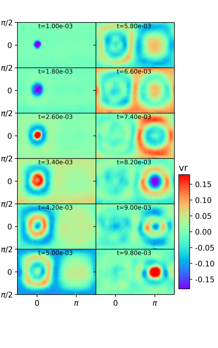
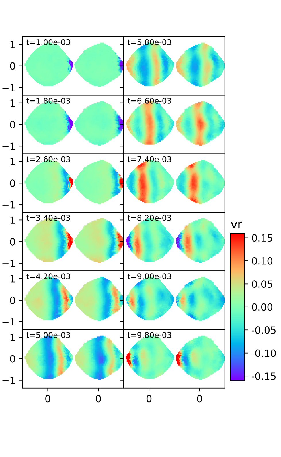
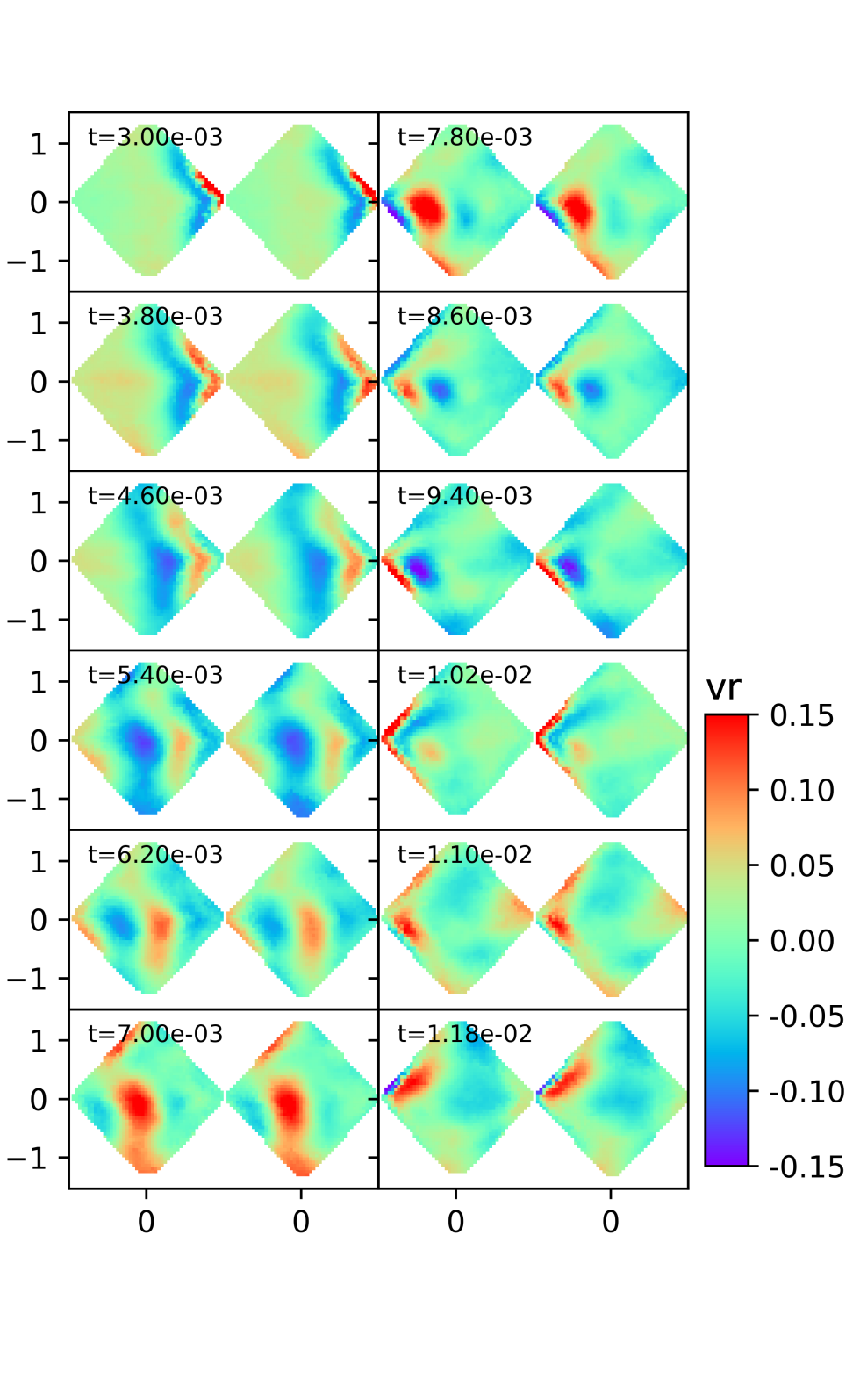
The mass-spring model approximates a homogeneous and isotropic elastic body in which elastic waves can propagate (Kot et al., 2015), however, we have not previously used it to simulate seismic waves. Tracking the motion of surface nodes only, we display the radial component of velocity as a function of time after impact for the Be0 simulation in Figure 4 using a cylindrical projection and in Figure 5 using front and back orthographic projections. These figures illustrate that a strong seismic pulse is excited by the impact that travels across the body surface. The impact occurs on the equator and at longitude $0^{\circ}$ and the simulated body is the Bennu shape model. The impulse is applied inward and so causes a negative radial velocity which appears blue in Figures 4 and 5. The second panel on the top left of 4 shows a blue ring propagating ahead of a red rebound moving outward away from the impact site. Seismic focusing (e.g., Schultz and Gault 1975; Meschede et al. 2011) is seen as the pulse becomes strong at the impulse’s antipode.

We estimate the time it takes the pulse to travel across the surface of the body. The pulse takes $\Delta t\approx 0.004$ to travel across 90 degrees in longitude or twice this $\sim 0.008$ to travel all the way to the other side of the body (to the impact’s antipode) where the wave is focused. Studies of antipodal focusing of seismic waves from an impact find that the main contribution to peak antipodal displacements comes from the constructive interference of low frequency Rayleigh waves (Schultz and Gault, 1975; Meschede et al., 2011). We estimate the Rayleigh wave speed from the Young’s modulus, P-wave speed and with Poisson ratio $\nu=1/4$, giving $V_{Ra}\approx 0.53\times 712=378$ in gravitational units, following our estimates in section §2.1 and parameters listed Table 1. To travel along the surface to the antipode, we estimate a time $t=\pi/V_{Ra}\approx\pi/378=0.0083$. The pulse travel time across the surface in the simulations is approximately consistent with the expected Rayleigh wave speed.

4.4 Spectrum of seismic waves excited by a simulated impact

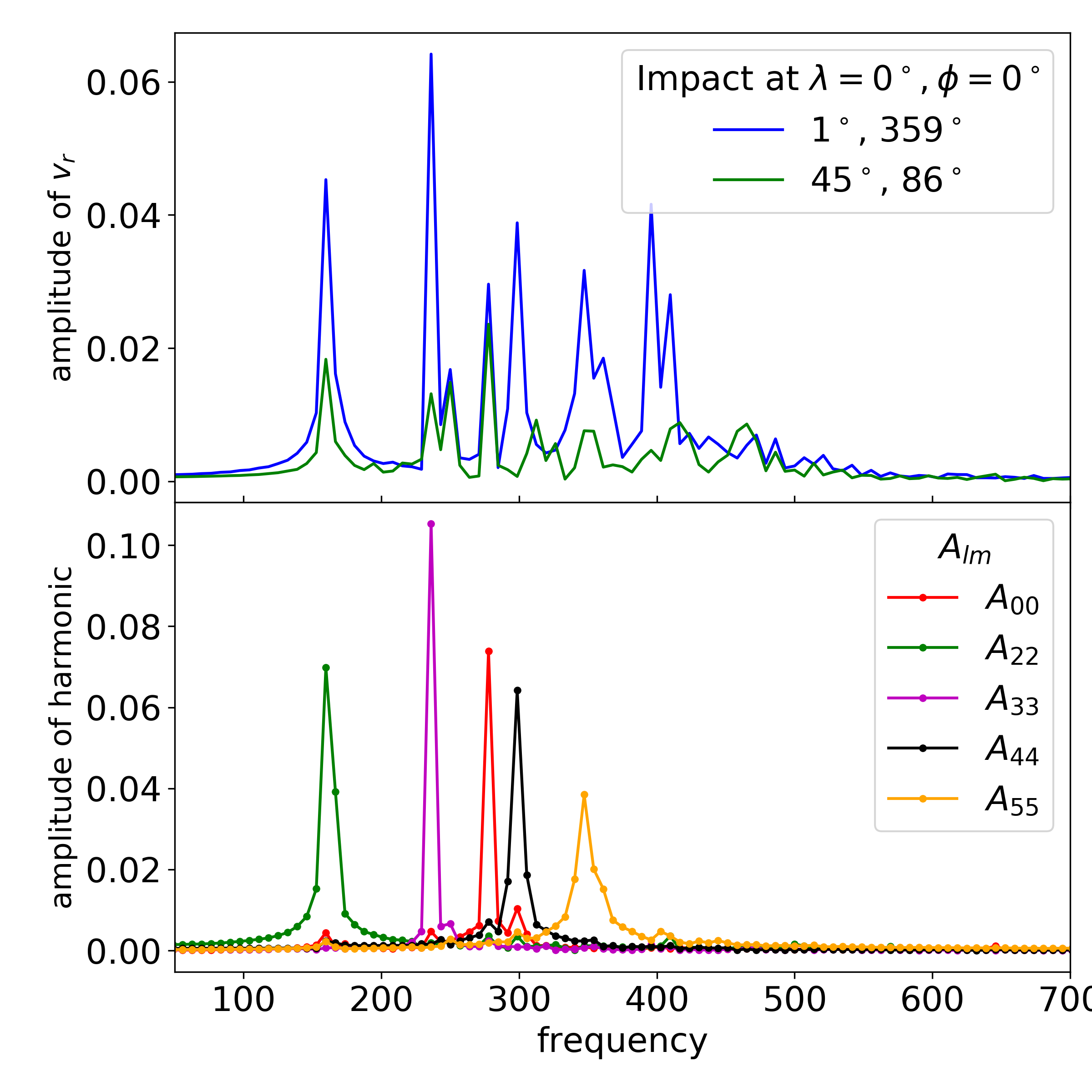
We examine the frequency spectrum of individual particle motions in the Be0 simulation. Using a fast Fourier transform, we compute the spectrum $\tilde{v}_{r}(f)=\int v_{r}(t)e^{i2\pi ft}dt$ from the particle’s radial velocity. We carry out the integral within a time window $\Delta t=0.15$ long and beginning just after the force pulse has ended. In Figure 6 top panel, we plot the amplitude $|\tilde{v}_{r}(f)|$ as a function of frequency for two surface particles, one near the equator and at longitude $\phi\approx 0^{\circ}$ and the other at a latitude of $\lambda\approx 45^{\circ}$ and longitude near $90^{\circ}$. The spectra in Figure 6 (top panel) are not flat but dominated by a series of peaks. A particle could be located at a node and so experience no vibration at an excited normal mode. This is why we plot the spectra of two particles at different locations so we are less likely to miss a strong frequency of vibration. Each peak in the spectra is associated with the normal modes defined by specific $l,n$ indices. Normal modes with the same $l,n$ but with different $m$ values should have similar frequencies as the body is nearly spherical.

Using spherical harmonics we identify which mode corresponds to each frequency peak and then discuss how well our mass spring model reproduces the normal mode frequencies that we predicted for a homogeneous elastic sphere.

On the surface of a nearly spherical body, the motions of a vibrational normal mode can be described with spherical harmonics,

$$Y_{l}^{m}(\theta,\phi)=\sqrt{\frac{2l+1}{4\pi}\frac{(l-m)!}{(l+m)!}}P_{l}^{m}(\cos\theta)e^{im\phi}$$ (31)

with spherical coordinate angles $\theta,\phi$. The azimuthal angle $\phi\in[0,2\pi]$ is equivalent to longitude and the inclination or colatitude angle $\theta\in[0,\pi]$ (with convention $\theta\equiv\pi/2-\lambda$). The functions $P_{l}^{m}(x)$ are Legendre polynomials. It is convenient to work with a real rather than complex set of functions,

$$Y_{lm}(\theta,\phi)=\left\{\begin{array}[]{c}Y_{l}^{m}(\theta,\phi)\\ \sqrt{2}(-1)^{m}{\rm Im}[Y_{l}^{|m|}(\theta,\phi)]\\ \sqrt{2}(-1)^{m}{\rm Re}[Y_{l}^{m}(\theta,\phi)]\end{array}\right.\qquad{\rm for}\qquad\begin{array}[]{c}m=0\\ m<0\\ m>0\end{array}.$$ (32)

The spherical harmonics are a complete set of orthonormal functions;

$$\int_{0}^{2\pi}d\phi\int_{0}^{\pi}\sin(\theta)d\theta\ Y_{lm}(\theta,\phi)Y_{l^{\prime}m^{\prime}}(\theta,\phi)=\delta_{mm^{\prime}}\delta_{ll^{\prime}}.$$ (33)

Using surface particles only we compute amplitudes of radial motions $v_{r}(\theta,\phi,t)$ with the integral

$$A_{lm}(t)=\int_{0}^{2\pi}d\phi\int_{0}^{\pi}d\theta\ Y_{lm}(\theta,\phi)v_{r}(\theta,\phi,t)$$ (34)

over the sphere. This gives us the amplitude as a function of time for each particular spherical harmonic with index $l,m$. We take the Fourier transform of $A_{lm}(t)$ with

$$\tilde{A}(f)=\int dtA_{lm}(t)e^{2\pi ift}.$$ (35)

The amplitude for 5 harmonics $|\tilde{A}_{lm}(f)|$ are plotted in Figure 6 for the same simulation as shown in Figures 4 and 5 but using simulation outputs extending to $t=0.15$ after impact. We don’t show the $l=1$ spherical harmonic as it would only show motion of the body’s center of mass. We compute the spectrum for $l=m$ spherical harmonics to make sure that $l$ nodes and anti-nodes are present on the equator, as our impact for this simulation took place on the equator. The Fourier transforms for each spherical harmonic amplitude $|\tilde{A}_{lm}|$ peaks at a single frequency. This frequency should be equivalent to that of normal modes with indices $l,n$ and with associated normal mode frequency ${}_{n}f_{l}$. We expect that the $l$ of the spherical harmonic is equal to the $l$ index of the normal mode.

Table 3: Peak Frequencies

Spherical harmonic	Peak of $|\tilde{A}_{lm}|$	Related mode	Expected frequency
$Y_{00}$	278	${}_{0}f_{0}$	292
$Y_{22}$	160	${}_{0}f_{2}$	148
$Y_{33}$	236	${}_{0}f_{3}$	208
$Y_{44}$	299	${}_{0}f_{4}$	268
$Y_{55}$	347	${}_{0}f_{5}$	329
Notes: The spherical harmonics are listed in the first column. The peak frequencies (in N-body or gravitational units) of the amplitudes for each spherical harmonic are measured for the Be0 simulation shown in Figures 4, 5, and 6 using the spectra shown in the bottom panel of Figure 6. The simulation has an equatorial impact on the Bennu shape model. The measured frequencies are listed in the second column. The relevant normal mode frequency is shown in the third column in the form ${}_{n}f_{l}$. The expected frequency of this mode for the same simulation is listed in the fourth column. These frequencies are computed following section §2.2 (equations 8 and 11) for a homogenous isotropic elastic sphere with a Poisson ratio of $\nu=1/4$ and P-wave speed of 712 in N-body units. The predicted and measured normal mode frequencies are similar implying that the mass-spring model simulations are behaving as expected.

In Table 3 we show the peak frequencies for the spherical harmonic amplitudes measured from the spectra in the bottom panel of Figure 6. These are in N-body units (in units of $t_{\rm grav}^{-1}$). In the same table we use the formulas given in section §2.2 (equations 8 and 11) to compute the expected frequencies of the normal modes, assuming a homogenous elastic sphere with a Poisson ratio of $\nu=1/4$ and P-wave speed of 712 in N-body units, matching that we estimated for the simulated elastic modulus.

A comparison between predicted and measured normal mode frequencies in Table 3 implies that the simulated Rayleigh wave speed is about 10% higher than we predicted for the simulation, as the $l>0$ modes have somewhat higher frequencies than we expect. The radial mode ${}_{0}f_{0}$ has frequency slower than we expected, so perhaps the P-wave speed is somewhat slower. Our simple elastic model exhibits normal modes and with frequencies near those we predict for a homogenous elastic sphere.

The spectrum shown in Figure 6 shows that the strongest modes excited by the simulated impact are the football mode with $l=2$, the triangular mode with $l=3$ and the radial $l=0$ mode. We chose the impulse source time, force amplitude and area so as to mimic an impact that we suspected would be in a regime capable of exciting slow normal modes. We have verified that predominantly slow normal modes were excited in the simulation. This was expected as we chose the impactor and its associated seismic source function to be in a regime consistent with excitation of the slowest normal modes.

Figure 6: The top panels shows the frequency spectrum of the radial velocity of two individual surface particles from the same simulation shown in Figures 4 and 5 of an equatorial impact on the Bennu shape model. The latitude and longitude of the two particles are shown in the key in the same panel. In the bottom panel we show the spectrum of different spherical harmonic amplitudes. These are measured using particles near the surface and with equations 34 and 35. Peaks in the spectra can be identified with the shapes of normal modes. The strongest normal modes excited by this simulated impact are the football mode $l=2$, the $l=3$ triangular mode and the radial $l=0$ mode. The seismic source duration was long enough to excite low frequency normal modes.

$\begin{array}[]{lll}\includegraphics[width=144.54pt,trim=40.15pt 10.03749pt 0.0pt 0.0pt,clip]{vr2ave_eq_long2.png}&\includegraphics[width=144.54pt,trim=40.15pt 10.03749pt 0.0pt 0.0pt,clip]{vr2ave_15_long2.png}&\includegraphics[width=144.54pt,trim=40.15pt 10.03749pt 0.0pt 0.0pt,clip]{vr2ave_65_long2.png}\end{array}$

Figure 7: We show the root mean square of radial motions $\sqrt{\langle v_{r}^{2}\rangle}$ for three sets of simulations averaged over a time of $\Delta t=0.09$ or 12 football normal mode oscillation periods. Axes for individual panels are longitude and latitude, however the longitude on the right hand side extends past $2\pi$ so that structure near the impact longitude can be more clearly seen. In top, middle and bottom panels we show impacts on Bennu, Cone and Oblate shape models. The left column shows equatorial impacts, the middle column shows impacts at a latitude of $15^{\circ}$ and the right column shows impacts at $15^{\circ}$. Impacts were at a longitude of $\phi=0^{\circ}$. The simulations are those listed in Table 2. The Bennu shape model shows peaks for low latitude impacts at $\phi\sim\pm\pi/2$ because the surface itself has four equatorial peaks.

Figure 8: We show a cartoon illustration of an impact hitting the equator of a body. The point of impact is represented by a star. On the left, the football ($l=2$) mode is excited giving four antinodes, shown as orange filled circles. In the middle panel, the triangular mode ($l=3$) is excited giving six antinodes (red circles). On the right panel we show the location of both sets of antinodes. The antinodes only coincide at impact and its antipodal point.

4.5 Patterns of surface motions

Because only a few normal modes are strongly excited in our simulations, vibrational motions on the surface are not evenly distributed. From particles near the surface we compute the root mean square of radial velocity variations $\sqrt{\langle v_{r}^{2}\rangle}$ by taking the average of $v_{r}^{2}$ for each particle from a series of simulation outputs. The patterns of radial velocity variations for nine simulations, using Bennu, Cone and Oblate shape models and for impacts at latitudes of 0, 15 and 65^∘ are shown in Figure 7. The parameters for the simulations are listed in Table 2. The $x$ axes are longitude and the $y$ axes are latitude. The longitude range exceeds $2\pi$ so that the pattern of vibrations near longitude $\phi=0$, where the impact took place, is easier to see. The portion of the surface on the far right of these figures is the same as that on the far left. To compute the averages for $\langle v_{r}^{2}\rangle$ we used simulation outputs spaced by 5 time steps or $10^{-4}$ and extending over a time period $\Delta t=0.09$. The time window is about 12 football mode ($l=2$) periods. The football mode is the slowest mode seen in our spectra. These figures show the vibrational energy distribution that might be experienced by the asteroid surface if the seismic waves are damped slowly. We note that the spring network only approximates a continuum elastic model, so on long time periods, coupling between modes may mimic seismic wave scattering.

The color bars in Figure 7 show the size of the radial velocities in N-body units. The sizes for $\sqrt{\langle v_{r}^{2}\rangle}\sim 0.05$ are not large, but they when integrated over the volume are approximately consistent with the total simulated seismic energy $E_{s}=0.004$ that we estimated for our pulse length and force amplitude using parameters from our simulations (listed in Table 2 and using equations 29 and 30).

We estimate the associated accelerations by multiplying the velocity $\sqrt{\langle v_{r}^{2}\rangle}$ by an angular oscillation frequency $\omega=2\pi f$. The frequency of the modes (in Table 3) range from $f=150$ to 300 in units of $t_{\rm grav}^{-1}$. The accelerations at the peaks are about 60 in N-body units, allowing seismic surface motions to launch material off the surface for short periods of time. Material is not ejected as the initial velocity of lofted material should not be larger than the maximum $v_{r}$ of the surface. The acceleration divided by the surface gravitational acceleration is sometimes called the acceleration parameter, $\Gamma$. We should not be surprised by the size of the acceleration parameter, as our simulated impact was chosen to be above the global seismic reverberation threshold with $\Gamma\sim 1$. Dividing $\sqrt{\langle v_{r}^{2}\rangle}$ by an angular frequency typical of the oscillation gives us the size of seismic displacements. The displacements are small, $\sim 10^{-4}$ in units of body radius, corresponding to 2.5 cm for Bennu’s radius.

Figure 7 shows a similarity between surface shape and the distribution of vibrational energy. The equatorial ridges in the Bennu model and bi-cone model simulations show higher levels of vibrational energy than mid latitudes, particularly for the low latitude impacts. The Bennu shape model shows four peaks in the vibrational energy distribution. We attribute this to the four peaks on its equatorial ridge. We know this is not due to the angular phases of the normal modes because the axisymmetric shape models don’t show the same four peaks.

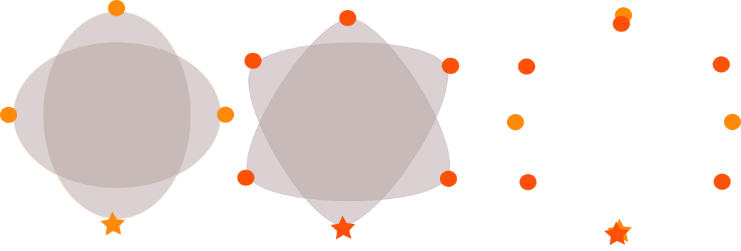
Although our spectra (discussed in section 4.4) show strong excitation of both football ($l=2$) and triangular $l=3$ spherical modes, we see the strongest vibrational motions at the impact sight and its antipodal point. Interference between $l=3$ and $l=2$ modes on the equator can reduce the strength of antinodes in the football modes that are $\pm 90^{\circ}$ from the impact point, see Figure 8 for an illustration. Also, due to excitation of different $m$ harmonics when excited at a single point, the football mode has power along the entire plane perpendicular to the impact point. This is seen in Figure 7 as a vertical bar at a longitude of $\phi\sim\pi$.

At an impact latitude of $15^{\circ}$, the morphology of vibrational energy is different than for an equatorial impact. Again peaks are seen at impact site and its antipode but these now lie above and below the equator. Associated surface slumping toward the equator would be lopsided. Impacts at higher latitudes cause little excitation near the equator.

Our vibrational energy maps of Figure 7 show that vibration tends to be more vigorous along the equator where surface elevation is highest. This is similar to a process known as ‘topographic amplification’ (e.g., Lee et al. 2009). We would predict, based on the vibration energy maps, that a near equatorial impact would preferentially cause surface slumping toward the equator and to a larger extent at impact site and its antipodal point. We do not see a single football mode excited that gives vibration preferentially at four equatorial peaks as are seen on Bennu’s equatorial ridge. The Bennu shape mode does show increased vibration at four peaks but that is because these locations are elevated and the normal modes themselves show more vibration at these points. Without elevation variations along the equator, as is true for our bi-cone and oblate models, four equatorial peaks are not seen in the vibration maps. If seismic waves are long-lasting, an impact is unlikely to explain the formation of the four peaks currently seen on Bennu’s equatorial ridge, from an initially axisymmetric ridge, unless the $l=3$ mode damps faster than the football mode.

If the simulated body has a harder core would the change in the normal mode frequencies allow four peaks to be seen? The $n=0$ modes can be described as constructively interfering Rayleigh waves propagating across the surface. The $l=2$ mode is comprised of a longer wavelength Rayleigh wave that penetrates deeper than the $l=3$ mode. With a harder core, we expect a faster $l=2$ mode. This would reduce the ratio of the $l=2$ and $l=3$ mode frequencies compared to that of a homogeneous body. With closer frequencies, both modes must simultaneously be excited. So an impact on a model with a hard core would not preferentially excite the football $l=2$ mode. And with closer frequencies, their damping rates would be similar.

$\begin{array}[]{lll}\includegraphics[width=144.54pt,trim=40.15pt 10.03749pt 0.0pt 0.0pt,clip]{max_eq_s.png}&\includegraphics[width=144.54pt,trim=40.15pt 10.03749pt 0.0pt 0.0pt,clip]{max_15_s.png}&\includegraphics[width=144.54pt,trim=40.15pt 10.03749pt 0.0pt 0.0pt,clip]{max_65_s.png}\end{array}$

Figure 9: Similar to Figure 7 except we show the maximum values of the radial velocity $v_{r}$ during a time $\Delta t=0.01$, approximately the time it takes the surface Rayleigh wave to focus on the impact antipode. Four equatorial peaks are seen in the bi-cone shape model for low latitude impacts.

If the seismic waves are rapidly damped, would we see different structure in the vibrational motions? In Figure 9 we plot the maximum (and positive) value of $v_{r}$ spanning the window of time $\Delta t=0.01$, from just after impulse has ended to just after the seismic pulse is focused at the antipode. Four or five equatorial peaks are seen for low latitude impacts. Four peaks are easiest to see in the bi-cone shape model simulations. We attribute the structure on the equatorial ridge of the bi-cone model to the non-spherical shape of the body, allowing moderate wavelength seismic waves to focus and constructively interfere on the equator. Figure 10 shows the wave front and is similar to Figure 5 but shows the C15 simulation using a bi-cone shape model and with a $15^{\circ}$ latitude impact. The wave front curvature is most easily seen in the left panels of Figure 10 and the resulting equatorial focusing on the equator and about $90^{\circ}$ from the impact sight is seen on the top right panel.

We notice that the equatorial peaks near $\pm\pi/2$ seen in the equatorial impacts in Figure 9 are not $180^{\circ}$ apart. The two weaker equatorial peaks on Bennu seem to be nearly $180^{\circ}$ apart (see Figure 2). Focusing of the seismic wave would be sensitive to body composition and shape, so a more complex model might produce peaks in a maximum $v_{r}$ map with locations similar to on Bennu’s equatorial ridge.

In summary, if seismic reverberations are long lasting, vibrational energy on the surface is primarily seen at impact point and its antipode. Regions of higher surface elevation (such as the equatorial ridge) show more vibration. We expect slumping toward the equator from impact site and its antipode. If seismic reverberations are quickly damped, then motions are highest in regions where the impact excited pulse is focused. In addition to the impact antipode, focus points could occur on the equatorial ridge for low-latitude impacts and near $90^{\circ}$ from the impact point.

Figure 10: Same as Figure 5 except showing the C15 simulation with a Cone shape model and a $15^{\circ}$ latitude impact site.

5 Vibration induced granular flows on the surface of Bennu

Above we have shown that surface vibrations caused by a large impact reflect the structure of vibrational normal modes, with some regions on the surface experiencing more shaking than others. We have also seen that the seismic pulse on a non-spherical body is not uniform in strength as it traverses the surface. In this section we explore how these two types of motions might induce granular flows on Bennu’s surface.

Spectral measurements and Bennu’s estimated thermal inertia imply that the surface of Bennu supports regolith that is comprised of grains with typical sizes between 1 mm and 1 cm (Emery et al., 2014). The equatorial ridge is redder than the poles, suggesting that the ridge material contains smaller grains that preferentially migrates to the geo-potential low (Binzel et al., 2015). Notably (Tardivel et al., 2018) predict the opposite trend, that deformation during spin-up would generate a rocky equator and sandy tropics. We lack constraints on the depth of Bennu’s regolith layer, however the asteroid porosity and near spherical shape (implying an absence of embedded monoliths) could be consistent with thick layers of regolith, subsurface rubble or porous and cracked rock. The depth of flow induced by vibration is likely to be smaller than the lateral dimensions of our problem so we restrict our discussion to surface flows (e.g., Aradian et al. 2002). This assumption neglects rearrangements deep inside the asteroid that could be caused by the passage of a seismic pulse.

Granular flows are complex, exhibiting a rich phenomenology even in the absence of vibration (e.g., Aranson and Tsimring 2002; Forterre and Pouliquen 2008). As the vibrational modes have periods similar to a Hz, if shape changes are caused by impacts, they must occur during a short time (a few hundred periods is only a few minutes). Significant mass flows, those large enough to change the body shape, are not possible in a short time unless the thickness of the flowing layer significantly exceeds the typical grain size. The granular flow must be in a dense and liquid-like state, similar to flows on inclined planes, rather than a gaseous or solid-like state where jamming and avalanches can take place. For discussion on granular flow regimes see Campbell ; Forterre and Pouliquen (2008).

Bennu’s surfaces exhibits downhill slopes (see Figures by Scheeres et al. 2016), so its surface material is not currently fluid-like. Bennu’s surface slopes are below the critical angle of repose of the granular medium on its surface. However, vigorous vibration can cause fluid-like behavior in a granular medium, or vibro-fluidization (e.g., Savage 1988), lowering the critical angle of the surface. We adopt a depth-averaged description for a surface flow, using variables similar to those used for Saint-Venant equations for shallow water waves that have been modified for granular flows (Savage and Hutter, 1989; Aradian et al., 2002; Forterre and Pouliquen, 2008). The advantage of this approach is that we don’t need to model the velocity profile in the flowing layer. We assume that there is a well defined interface between a flowing layer and static underlying material. We describe the flow with a thickness for the flowing layer, $h$, and ${\bf u}$ a depth averaged velocity in the flowing layer, giving mass flux ${\bf Q}=\rho h{\bf u}$ (see section 4 by Forterre and Pouliquen 2008 or Aradian et al. 2002). Conservation of mass is described with

$$\frac{\partial h}{\partial t}+{\boldsymbol{\nabla}}\cdot\left(h{\bf u}\right)=\frac{\partial H}{\partial t}.$$ (36)

We have assumed an incompressible medium. The divergence is restricted to gradients on the surface. With $\frac{\partial H}{\partial t}=0$, there is no exchange between the surface flow and the underlying static base. If there is mass exchange, the static base increases or decreases in height at a rate given by $\frac{\partial H}{\partial t}$.

At each location on the surface the mass flux ${\bf Q}$ should depend on the surface gravitational acceleration, $g_{\rm geo}=|{\bf a}_{\rm geo}|$, the slope of the surface $\beta$, the amplitude of seismic vibrations characterized by the mean $\langle v_{r}^{2}\rangle$ or the maximum $v_{r}$ during the seismic pulse, and the depth of the flowing layer $h$. Here ${\bf a}_{\rm geo}$ is the direction of acceleration on the surface due to gravity and body spin. We assume that the flow velocity ${\bf u}$ is in the downhill direction, that given by the gradient of the geopotential on the surface. The flow rate $u$ and mass flux $\rho h{\bf u}$ should increase with increasing surface slope, vibration velocity, and decreasing surface gravity.

We explore two types of models, a hopping block model with flowing layer depth $h$ independent of position on the surface and a fluidized layer model with $h$ set by the level of vibrations. The hopping block model is similar to the hopping and sliding block model (slipping with friction) used by Richardson et al. (2005) to estimate surface flows caused by seismic reverberation. The average flow velocity $u$ varies with position on the surface for both models.

In section §5.1 we compute the surface slope, as flow rates should depend on it. In section §5.2 we consider a hopping block model with a depth $h$ for the flowing layer that is independent of surface position. The model is computed for flow caused by a seismic pulse (dependent on max $v_{r}$) and for prolonged seismic reverberation (and dependent on $\langle v_{r}^{2}\rangle$). In section §5.3 we use the notion of granular temperature to estimate a depth $h$ for vibro-fluidization and an empirical flow rule for granular flows on inclined planes to estimate a depth-averaged velocity ${\bf u}$ in the flowing layer. In section §5.4 these three models are used to estimate the distribution, rate and extent that flowing granular material is accumulated on the surface due to an energetic impact.

5.1 Surface acceleration and slope

To estimate surface flows we need to compute the vertical acceleration at the surface for an aspherical and spinning body. The geopotential is defined as

$$\Phi_{\rm geo}({\bf r})\equiv-\frac{1}{2}\Omega^{2}(x^{2}+y^{2})-U({\bf r})$$ (37)

(following Scheeres et al. 2016 for $z$-axis, spin axis and a body principal axis aligned) where ${\bf r}=(x,y,z)$ are coordinates in the body frame with respect to the center of mass, $\Omega$ is the body’s spin rate and $U({\bf r})$ is the gravitational potential energy per unit mass; $U({\bf r})=\int d^{3}{\bf r}^{\prime}\rho({\bf r}^{\prime})|{\bf r}-{\bf r}^{\prime}|^{-\frac{1}{2}}$. We compute a local gravitational acceleration vector at a surface position ${\bf r}_{s}$

$${\bf a}_{\rm geo}({\bf r}_{s}) =\left.{\boldsymbol{\nabla}}\Phi_{\rm geo}({\bf r})\right|_{{\bf r_{s}}}$$ (38)

where the gradient is computed in three-dimensions and then evaluated at a point on the surface ${\bf r}_{s}$.

A surface slope is the relative orientation between the surface normal vector and the local gravitational acceleration vector. We describe the surface slope with an angle $\beta_{\rm slope}$, with

$$\sin\beta_{\rm slope}({\bf r}_{s})=\frac{{\bf a}_{\rm geo}({\bf r}_{s})\cdot\hat{\bf n}({\bf r}_{s})}{|{\bf a}_{\rm geo}({\bf r}_{s})|}$$ (39)

and with $\hat{\bf n}({\bf r}_{s})$ a unit vector normal to the surface. The slope angle $\beta_{\rm slope}=0$ if surface normal and gravitational acceleration vectors are aligned.

5.2 Hopping model

At acceleration parameter greater than 1 (with accelerations due to vibration exceeding the surface acceleration), particles on the surface are pushed off the surface into free fall. A particle that is launched from the surface with vertical velocity $v$ is in flight for a time $\Delta t=2v/g_{\rm geo}$. With a surface slope $\beta$, the particle travels downhill horizontally a distance $\Delta x\sim v\beta\Delta t\sim 2\beta v^{2}/g_{\rm geo}$ or at an average horizontal speed $u\sim\Delta x/\Delta t\sim v\beta$. Here the notion of horizontal and vertical are with respect to the gravitational acceleration vector.

For long timescale seismic reverberation we estimate the vertical velocity $v$ using the root mean square of radial velocity variations $\sqrt{\langle v_{r}^{2}\rangle}$, giving an average horizontal velocity

$$u\sim\beta\sqrt{\langle v_{r}^{2}\rangle}.$$ (40)

We assume flow is downhill, which we denote with a vector on the surface $\hat{\boldsymbol{\beta}}$. With a constant depth $h$ of flowing material equation 36 gives a rate the surface elevation changes

$$\frac{1}{h}\frac{\partial H({\bf r}_{s})}{\partial t}\approx{\boldsymbol{\nabla}}\cdot\left(\beta\hat{\boldsymbol{\beta}}\sqrt{\langle v_{r}^{2}\rangle}\right)$$ (41)

at a position ${\bf r}_{s}$ on the surface, with quantities on the right hand side dependent on surface position ${\bf r}_{s}$ and with the gradient operator applied on the surface.

For a seismic surface pulse (and assuming that the seismic waves damp quickly) we estimate the distance traveled on the surface $\Delta x$ from the maximum outward velocity $v_{r}$ and with a single hop (and no slip), giving

$$\Delta x\sim\frac{2\beta|{\rm max}v_{r}|^{2}}{g_{\rm geo}}.$$ (42)

With a constant depth $h$ of flowing material, equation 36 for conservation of mass gives a total height change following a seismic pulse

$$\frac{\Delta H({\bf r}_{s})}{h}\approx{\boldsymbol{\nabla}}\cdot\left(\frac{2\beta\hat{\boldsymbol{\beta}}|{\rm max}v_{r}|^{2}}{g_{\rm geo}}\right).$$ (43)

and with quantities on the right hand side dependent on surface position ${\bf r}_{s}$.

5.3 Vibro-fluidization flow model

Kinetic theories for granular flow are often dependent on the notion of a granular temperature (Ogawa et al., 1980; Jenkins and Savage, 1983; Lun et al., 1984; Ding and Gidaspow, 1990; Warr et al., 1995; Goldhirsch, 2008) that is estimated from the square of velocity fluctuations in the grains. In a vibrating granular bed, the granular temperature is proportional to the root mean square of the velocity of vibrations (Warr et al., 1995; Kumaran, 1998). Following scaling by Kumaran (1998) for media with weak dissipation (little friction), we assume the granular temperature

$$T_{\rm granular}({\bf r}_{s})\approx\langle v_{r}^{2}({\bf r}_{s})\rangle,$$ (44)

where $\langle v_{r}^{2}({\bf r}_{s})\rangle$ represents a time integrated average of the velocity fluctuations caused by seismic vibrations. The granular temperature gives an estimate for a pressure associated with vibrational kinetic energy, $P_{\rm kinetic}=\rho T_{\rm granular}$. We compare the kinetic pressure to hydrostatic pressure $\rho g_{\rm geo}h$ at a depth $h$ where $g_{\rm geo}\approx|{\bf a}_{\rm geo}|$ is the acceleration near the surface due to gravity and body spin. Equating hydrostatic pressure at depth $h$ to that associated with vibrational motions gives an approximate depth for the base of a vibro-fluidized layer,

$$h({\bf r}_{s})\approx\frac{\langle v_{r}^{2}({\bf r}_{s})\rangle}{g_{\rm geo}({\bf r}_{s})}.$$ (45)

This estimate for depth assumes that a significant fraction of the vibrational energy goes into random grain motions. If the grain motions are correlated then the fluidized layer would be deeper than estimated by equation 45.

What size does equation 45 give for our impact simulations? Figure 7 shows peaks with $\langle v_{r}^{2}\rangle\sim 10^{-2}$ in N-body units. In our N-body units, acceleration for a non-rotating spherical body is 1. At the equator the surface gravity is about 1/2 of that without rotation, so equation 45 gives $h\sim 0.02$ in units of radius. For Bennu this corresponds to a depth of 5 m. The ratio of fluidization depth to grain size (using grains of size 0.3 cm) is $\sim 170$, exceeding many experiments but large enough that a shallow water wave analogy is appropriate.

If the depth of the fluidized layer $h$ is set by the vibrational kinetic energy, there is exchange between flowing material and the underlying medium. Ignoring slow variations in the time averaged vibrational energy, equation 36 becomes

$$\frac{\partial H({\bf r}_{s})}{\partial t}={\boldsymbol{\nabla}}\cdot\left[h({\bf r}_{s}){\bf u}({\bf r}_{s})\right].$$ (46)

With a relation for the flow velocity ${\bf u}$, this equation gives us an estimate for how granular flow on the surface increases or decreases the local surface height.

When described in terms of a continuum model, dense flows exhibit shear-rate dependent stress giving the flow a viscous-like behavior (Bagnold, 1954; Aradian et al., 2002; Aranson and Tsimring, 2002; Forterre and Pouliquen, 2008; Holsapple, 2013). Gravitational acceleration gives a component of the pressure gradient that is parallel to the surface and depends on the surface slope. A description for the vertical velocity profile of a flow and an effective flow viscosity (which could be depend on the shear as in the Bagnold description) gives a relation between averaged flow velocity and surface slope. Experiments and numerical simulations of steady granular flows on inclined planes (Pouliquen, 1999; Silbert et al., 2003.; GDR MiDi, 2004; Deboeuf et al., 2006) support an empirical flow rule relating the flow rate to the surface slope,

$$\frac{u}{\sqrt{g_{\rm geo}h}}\sim f(\beta).$$ (47)

The quantity on the left $u/\sqrt{g_{\rm geo}h}$ can be identified as a Froude number making the function $f()$ dimensionless. With equation 45 for $h$, $u\propto\sqrt{g_{\rm geo}h}=\sqrt{\langle v_{r}^{2}\rangle}$ and is dependent on the root mean square of vibrational velocity and consistent with the estimate we derived for hopping in equation 40. The function $f(\beta)$ depends on slope and grain properties such as packing fraction and the critical angle of repose of the granular medium, $\beta_{c}$. Unfortunately the empirical scaling laws for steady flow on inclined planes neglect vibration. Without vibration and with slope $\beta<\beta_{c}$ below the critical angle of repose, there would be no flow. For our vibro-fluidized layer we modify the scaling relation of equation 47 that is successful at describing granular flows on inclined planes. We desire a function $f()$ that gives a more flow at higher slopes and no flow when the slope is zero. A linear function does this

$$f(\beta)=K\beta$$ (48)

with $K$ a unitless scaling factor.

Combining equations 45, 46, 47, and 48 we estimate the height increase or decrease due to impact excited vibrations

$$\frac{\partial H({\bf r}_{s})}{\partial t}\sim{\boldsymbol{\nabla}}\cdot\left[K\beta\hat{\boldsymbol{\beta}}\frac{\langle v_{r}^{2}\rangle^{\frac{3}{2}}}{g_{\rm geo}}\right]$$ (49)

with the gradient restricted to the surface and quantities on the right hand side (excepting $K$) that are functions of surface position ${\bf r}_{s}$. Despite the uncertainties in estimating the flow of vibrated granular materials this equation shows expected trends. There is more flow where there is more vibration, such as at antinodes. There is no flow predicted where the surface slope is zero and there is more flow where surface acceleration is lower at the equator. While the direction of flow is toward the equator, height changes can occur non-uniformly in azimuth because the vibrational energy depends on longitude.

$\begin{array}[]{lll}\includegraphics[width=144.54pt,trim=40.15pt 10.03749pt 0.0pt 0.0pt,clip]{grad_eq_short.png}&\includegraphics[width=144.54pt,trim=40.15pt 10.03749pt 0.0pt 0.0pt,clip]{grad_15_short.png}&\includegraphics[width=144.54pt,trim=40.15pt 10.03749pt 0.0pt 0.0pt,clip]{grad_65_short.png}\end{array}$

Figure 11: Estimates for the change in surface height divided by flow layer depth, $\Delta H/h$, for a seismic jolt one hop model caused by energetic impacts. The height changes are estimated using the maximum positive $v_{r}$ shown in Figure 9 from the initial seismic pulse and equation 43 for the height change divided by depth of flowing layer. As before, we show nine simulations, for three different impact latitudes (left to right) and three different shape models (top to bottom).

$\begin{array}[]{lll}\includegraphics[width=151.76744pt,trim=40.15pt 10.03749pt 0.0pt 0.0pt,clip]{grad_eq_ch.png}&\includegraphics[width=151.76744pt,trim=40.15pt 10.03749pt 0.0pt 0.0pt,clip]{grad_15_ch.png}&\includegraphics[width=151.76744pt,trim=40.15pt 10.03749pt 0.0pt 0.0pt,clip]{grad_65_ch.png}\end{array}$

Figure 12: Estimates for the rate of change of surface height divided by flow layer depth, $\frac{1}{h}\frac{\partial H}{\partial t}$ long lasting seismic reverberations and a constant depth flow model. The height changes are estimated using $\langle v_{r}^{2}\rangle$ shown in Figure 7 and equation 41 for our nine simulations.

$\begin{array}[]{lll}\includegraphics[width=151.76744pt,trim=40.15pt 10.03749pt 0.0pt 0.0pt,clip]{grad_eq_long.png}&\includegraphics[width=151.76744pt,trim=40.15pt 10.03749pt 0.0pt 0.0pt,clip]{grad_15_long.png}&\includegraphics[width=151.76744pt,trim=40.15pt 10.03749pt 0.0pt 0.0pt,clip]{grad_65_long.png}\end{array}$

Figure 13: Estimates for the rate of change of surface height, $\frac{\partial H}{\partial t}$ long lasting seismic reverberations and a vibro-fluidization flow model. The height changes are estimated using $\langle v_{r}^{2}\rangle$ shown in Figure 7 and equation 49 with $K=1$ for our nine simulations.

5.4 Surface height changes

We have three estimates for surface height variations, a seismic jolt one hop model, and two seismic reverberation models. The seismic jolt one hop model uses the maximum positive radial velocity $v_{r}$ shown in Figure 9 and equation 43 for the change in surface height to produce Figure 11, showing $\Delta H/h$ for our nine simulations. The seismic pulse exhibited by our simulations primarily give strong equatorial flows, however four peaks are seen on the equator in bi-cone and oblate models with near equatorial impacts. The color bar scale shows $\Delta H/h$ so the size of the variations in height are less than 1/4 of the depth of the flowing layer $h$. Figure 2 shows that the peak to peak elevation differences on Bennu are $\Delta H\sim 1/10$ of its radius. To match these height variations we would require a flow depth $h$ to be similar to 0.4 times the radius of Bennu itself. This implies that focusing of the initial seismic could not account for Bennu’s 4 equatorial peaks.

The first of our seismic reverberation models assumes a constant depth for the flowing layer and estimates the flow rate using a typical hop speed. For this model we use $\langle v_{r}^{2}\rangle$ shown in Figure 7 and equation 41 to produce Figure 12, showing $\frac{1}{h}\frac{\partial H}{\partial t}$ for our nine simulations. These figures show accumulation at the equatorial ridge, impact point and its antipode. To estimate the height change $\Delta H$ we must multiply by the total length of time of seismic reverberation. A value of 2000 times the frequency of the $l=2$ normal mode gives a time $\Delta t=14$ in gravitational units. Here 2000 is a $Q$ value for the ratio of energy lost per cycle. Taking a maximum value of $\frac{1}{h}\frac{\partial H}{\partial t}\approx 0.3$ we estimate a total height change of $\Delta H\approx 4h$. If the depth of flowing material is a few meters then the equatorial ridge could increase by $\sim 10$ meters.

The second of our seismic reverberation models assumes a fluidization depth estimated with a granular temperature and a flow rate with scaling motived by studies of inclined plane granular flow. For prolonged seismic reverberations, we use $\langle v_{r}^{2}\rangle$ shown in Figure 7 and equation 49 with $K=1$ to produce Figure 13, showing $\frac{\partial H}{\partial t}$ for our nine simulations. To estimate the height change $\Delta H$ we must multiply by the total length of time of seismic reverberation. Taking a maximum value of $2\times 10^{-3}$ for $\frac{\partial H}{\partial t}$ times a time 14 (corresponding to a $Q$ of 2000 times the period of the $l=2$ mode) we estimate $\Delta H\approx 0.03$ in units of body radius. This corresponds to 7 meters on Bennu. The scaling factor $K$ can exceed 1 and we may have underestimated the fluidization depth, so larger elevation gains might be possible.

In summary, a seismic jolt and hopping surface model seems unlikely to account for formation of Bennu’s four equatorial peaks. Prolonged seismic reverberation could cause an equatorial ridge or other high elevation regions to increase in height by a few meters. Impact point and its antipode could also increase in height by a few meters.

6 Discussion and Conclusions

Impacts that are above global seismicity thresholds for resurfacing and cause crater erasure likely happened on asteroids such as Bennu. These subcatastrophic impacts form large craters and should radiate seismic waves efficiently at low frequencies, thus they could couple to the normal modes of whole body. Low frequency seismic waves would damp less quickly than high frequency ones. If the attenuation rate is low, once low frequency normal modes are excited, the body may oscillate for many oscillation periods. But as the normal mode motions are not uniformly distributed on the body surface, the pattern of seismic reverberation depends on the structure of the normal modes themselves.

Because of the large seismic source size (because a large crater is formed) the initial surface impulse (or seismic jolt) contains power at long wavelengths and so can be focused by the shape of the body. Whether the seismic response decays rapidly or slowly giving a long period of seismic reverberation, the distribution of excited seismic motions would not be uniform across the surface.

We identify a regime in small asteroids less than a kilometer diameter where rare and subcatastrophic are above that giving global seismic reverberation. These impacts could excite low frequency normal modes. As the associated accelerations are well above that of surface gravity, the surface of the body could preferentially be modified where the excited normal modes or the initial seismic pulse is strongest. For the asteroid Bennu, a few meter diameter impactor could be in this regime.

We simulate excitation of seismic waves by an impact using a mass-spring elastic N-body model. The simulations let us explore the distribution of vibrational excitation on the surface for different asteroid shape models. The seismic source is modeled as a force applied to surface particles in a small region that has amplitude and time length estimated via scaling for a 4m diameter impactor on Bennu. We explore impacts on three shape models, the Bennu shape model, a bi-cone model with an equatorial ridge and an oblate model. Spectra of particle motions show that low frequency normal modes are excited, including the $l=2$ football-shaped spherical mode and the triangular-shaped $l=3$ normal mode. With a few thousand particles the mass-spring model shows normal modes at frequencies within 10% of those predicted for a homogeneous isotropic elastic sphere.

We use our simulations of impacts to display the root mean square of radial motions on the surface and the maximum positive radial speed caused by the initial seismic pulse. If seismic reverberations are prolonged, vibrational energy on the surface is primarily seen at impact point and its antipode. Regions of higher surface elevation (such as the equatorial ridge) show more vibration. Interference between excited $l=2$ and $l=3$ normal modes prevents points on the equator other than the impact point and its antipode from experiencing strong vibration. Bennu’s four equatorial would not be formed via seismic reverberation from an initially axisymmetric equatorial ridge.

If seismic reverberations are quickly damped, then motions are highest in regions where the impact excited pulse is focused. In addition to the impact antipode, focus points could occur on the equatorial ridge for low-latitude impacts and near $90^{\circ}$ from the impact point. Four equatorial peaks could be formed due to surface slumping but each one need not have an antipodal counter part, as is true for the Bennu shape mode by Nolan et al. (2013).

We explored three simple flow models. We estimated flow distance using a single hop and using a constant depth for a mobile layer. The hop distance was estimated from the highest positive radial velocity seen in the simulations on the surface. The estimated surface height variations were small and rule out a seismic impulse as a mechanism for forming four peaks on Bennu’s equatorial ridge. Our second flow model assumes prolonged seismic reverberation, adopts a velocity based on the acceleration parameter (and is equivalent to the average velocity during a hop) and assumes a constant depth for the mobile layer. Our third model also assumes prolonged seismic reverberation, but allows the depth of the mobile layer to depend on the level of surface vibration. With a long timescale for the decay of seismic energy (seismic $Q\sim 2000$), an energetic impact could cause shape changes of a few meters on an asteroid like Bennu. Primarily we see an increase in the height of an equatorial ridge, the point of impact and its antipode. If impact point is near but not on the equator, slumping toward the equator would be lopsided. In other words, flows toward the equator would preferentially happen from northern latitudes near the impact point and southern latitudes at its antipode, for an impact at a northern latitude. Four equatorial peaks are not formed due to interference between the excited $l=2$ (football shaped) and $l=3$ (triangular shaped) normal modes. This rules out an impact related prolonged seismic reverberation mechanism for the formation of Bennu’s 4 equatorial peaks.

Bennu’s 4 equatorial peaks are still a puzzle. Perhaps a tidal excitation would better excite the football-shaped mode without exciting an $l=3$ triangular mode, though a nearby encounter with a larger body would be required (e.g., see Press and Teukolsky 1977; Yu et al. 2014; Quillen et al. 2016a). Alternatively perhaps an excited $l=3$ triangular mode would decay more quickly than the football-shaped mode letting the body surface slump at four rather than two equatorial peaks. The four peaks may reflect a ‘ring-down’ in vibrational energy, similar to that of a bell. An abrupt earthquake along an internal fault could preferentially excite the football shaped normal mode. High resolution imaging of imaging that will be obtained by OSIRIS-REx will improve the shape model, confirming or refuting the existence of these peaks.

Here we adopted a wave speed typical of lunar regolith (as have some other asteroid seismic studies; Murdoch et al. 2017) and with Young’s modulus of 11 MPa. If there are large fractured blocks inside the asteroid, then the wave speed could be higher or the normal modes of the asteroid could be influenced by the normal mode spectrum of the blocks (e.g., Richardson et al. 2005). Cohesion models for asteroid estimate a strength about $10^{2}$–$10^{4}$ times weaker than 11 MPa (Sánchez and Scheeres, 2014; Scheeres and Sánchez, 2018). Even a cohesionless material should transmit a compression wave, but the wave rebound or reflection from surfaces would be reduced because the medium would deform under tension or loft particles off the surface rather than transmit a pulse. The difference emphasizes that we have used an elastic model, comprised of masses and springs, to explore the behavior of a body that could be a conglomerate.

Seismic attenuation, dispersion and scattering properties are not known for asteroids, and granular flow problems are complex even without high levels of subsurface vibration. It is not easy to predict whether granular material on a vibrating Chladni plate collects at anti-nodes or at nodes (e.g., Chladni 1787; Dorrestijn et al. 2007). We have neglected seismic attenuation and scattering, and our flow models are simplistic as they do not depend on nature of friction between particles and the particle size distribution (e.g., Richardson et al. 2005). We have neglected the details of crater formation, crater depth, re-accumulation of crater ejecta and have used a simple model for the seismic pulse generated by the impact. The amplitude of surface motions may depend on topography and sub-surface composition. (e.g., Kawase 1996; Lee et al. 2009) and the medium itself may be transformed or deformed by the passage of a pressure wave. Future studies of the strong impact regime considered here could improve upon our numerical techniques, and adopt more realistic asteroid composition, impact and flow models.

Bibliography

- Aki and Richards (2002) Aki, K., Richards, P., 2002. Quantitative Seismology, 2nd edition. University Science Books, Sausalito, CA.
- Aradian et al. (2002) Aradian, A., Raphaël, E., de Gennes, P.G., 2002. Surface flows of granular materials: a short introduction to some recent models. Compte Rendue Physique 3, 187–196.
- Aranson and Tsimring (2002) Aranson, I.S., Tsimring, L.S., 2002. Continuum theory of partially fluidized granular flows. Physics Review Letters 65, 061303.
- Asphaug (2008) Asphaug, E., 2008. Critical crater diameter and asteroid impact seismology. Meteoritics & Planetary Science 43, 1075–1084.
- Bagnold (1954) Bagnold, R.A., 1954. Experiments on a gravity-free dispersion of large solid particles in a newtonian fluid under shear. Proceedings of the Royal Society of London, Series A 225, 49–63.
- Benz and Asphaug (1999) Benz, W., Asphaug, E., 1999. Catastrophic disruptions revisited. Icarus 142, 5–20.
- Binzel et al. (2015) Binzel, R.P., DeMeo, F.E., Burt, B.J., Cloutis, E.A., Rozitis, B., Burbine, T.H., Campins, H., Clark, B.E., Emery, J.P., Hergenrother, C.W., Howell, E.S., Lauretta, D.S., Nolan, M.C., Mansfield, M., Pietrasz, V., Polishook, D., Scheeres, D.J., 2015. Spectral slope variations for osiris-rex target asteroid (101955) bennu: Possible evidence for a fine-grained regolith equatorial ridge. Icarus 256, 22 – 29. URL: http://www.sciencedirect.com/science/article/pii/S0019103515001463, doi:https://doi.org/10.1016/j.icarus.2015.04.011.
- Bottke et al. (1994) Bottke, W.F., Nolan, M., Greenberg, R., Kolvoord, R., 1994. Velocity distributions among colliding asteroids. Icarus 107, 255–268.
- (9) Campbell, C.S., . Rapid granular flows. Annual Review of Fluid Mechanics 22, 57–92.
- Cheng et al. (2002) Cheng, A.F., Izenberg, N., Chapman, C., Zuber, M., 2002. Ponded deposits on asteroid 433 eros. Meteoritics & Planetary Science 37, 1095–1105.
- Chesley et al. (2014) Chesley, S.R., Farnocchia, D., Nolan, M.C., Vokrouhlický, D., Chodas, P.W., Milani, A., Spoto, F., Rozitis, B., Benner, L.A., Bottke, W.F., Busch, M.W., Emery, J.P., Howell, E.S., Lauretta, D.S., Margot, J.L., Taylor, P.A., 2014. Orbit and bulk density of the osiris-rex target asteroid (101955) bennu. Icarus 235, 5 – 22. URL: http://www.sciencedirect.com/science/article/pii/S0019103514001067, doi:https://doi.org/10.1016/j.icarus.2014.02.020.
- Chladni (1787) Chladni, E.F.F., 1787. Entdeckungen über die Theorie des Klanges. Breitkopf und Härtel, Leipzig.
- Cintala et al. (1978) Cintala, M.J., Head, J.W., Veverka, J., 1978. Characteristics of the cratering process on small satellites and asteroids, in: Lunar and Planetary Science Conference Proceedings, pp. 3803–3830.
- Clark et al. (2012) Clark, A.H., Kondic, L., Behringer, R.P., 2012. Particle scale dynamics in granular impact. Physics Review Letters 109, 238302.
- Colwell et al. (2005) Colwell, J.E., Gulbis, A.A., Horányi, M., Robertson, S., 2005. Dust transport in photoelectron layers and the formation of dust ponds on eros. Icarus 175, 159 – 169. URL: http://www.sciencedirect.com/science/article/pii/S0019103504003847, doi:https://doi.org/10.1016/j.icarus.2004.11.001.
- Cooper et al. (1974) Cooper, M.R., Kovach, R.L., Watkins, J.S., 1974. Lunar near-surface structure. Reviews of Geophysics and Space Sciences 12, 291–308.
- Cundall and Strack (1979) Cundall, P.A., Strack, O.D.L., 1979. A discrete numerical model for granular assemblies. Geotechnique 29, 47–65.
- Dainty et al. (1974) Dainty, A., Toksöz, M.N., Anderson, K., Pines, P., Nakamura, Y., Latham, G., 1974. Seismic scattering and shallow structure of the moon in oceanus procellarum. Moon 9, 11–29.
- Deboeuf et al. (2006) Deboeuf, S., Lajeunesse, E., Dauchot, O., Andreotti, B., 2006. Flow rule, self-channelization and levees in unconfined granular flows. Physics Review Letters 97, 158303.
- Ding and Gidaspow (1990) Ding, J., Gidaspow, D., 1990. A bubbling fluidization model using kinetic theory of granular flow. AIChE Journal 36, 523–538. URL: http://dx.doi.org/10.1002/aic.690360404, doi:10.1002/aic.690360404.
- Dorrestijn et al. (2007) Dorrestijn, M., Bietsch, A., Acikalin, T., Raman, A., Hegner, M., Meyer, E., Gerber, C., 2007. Chladni figures revisited based on nanomechanics. Physics Review Letters 98, 026102.
- Duffy and Mindlin (1957) Duffy, J., Mindlin, R., 1957. Stress strain relations and vibrations of granular media. Journal of Applied Mechanics 24, 585–593.
- Emery et al. (2014) Emery, J., Fernández, Y., Kelley, M., (nèe Crane), K.W., Hergenrother, C., Lauretta, D., Drake, M., Campins, H., Ziffer, J., 2014. Thermal infrared observations and thermophysical characterization of osiris-rex target asteroid (101955) bennu. Icarus 234, 17 – 35. URL: http://www.sciencedirect.com/science/article/pii/S0019103514000827, doi:https://doi.org/10.1016/j.icarus.2014.02.005.
- Forterre and Pouliquen (2008) Forterre, Y., Pouliquen, O., 2008. Flows of dense granular media. Annual Review of Fluid Mechanics 40, 1–24.
- Freund (1998) Freund, L.B., 1998. Dynamic Fracture Mechanics. Cambridge University Press, Cambridge, England.
- Frouard et al. (2016) Frouard, J., Quillen, A.C., Efroimsky, M., Giannella, D., 2016. Numerical simulation of tidal evolution of a viscoelastic body modelled with a mass-spring network. Monthly Notices of the Royal Astronomical Society 458, 2890–2901.
- GDR MiDi (2004) GDR MiDi, 2004. On dense granular flows. The European Physical Journal E 14, 341–365. URL: https://doi.org/10.1140/epje/i2003-10153-0, doi:10.1140/epje/i2003-10153-0.
- Geng et al. (2001) Geng, J., Howell, D., Longhi, E., Behringer, R., Reydellet, G., Vanel, L., Clément, E., Luding, S., 2001. Footprints in sand: The response of a granular material to local perturbations. Physics Review Letters 87, 035506.
- Goldhirsch (2008) Goldhirsch, I., 2008. Introduction to granular temperature. Powder Technolology 182, 130–136.
- Greenberg et al. (1996) Greenberg, R., Bottke, W., M., N., Geissler, P., Petit, J., Durda, D., Asphaug, E., Head, J., 1996. Collisional and dynamical history of ida. Icarus 120, 106–118.
- Greenberg et al. (1994) Greenberg, R., Nolan, M., Bottke, W., Kolvoord, R., Veverka, J., 1994. Collisional history of gaspra. Icarus 107, 84–97.
- Guibout and Scheeres (2003) Guibout, V., Scheeres, D., 2003. Stability of surface motion on a rotating ellipsoid. Celestial Mechanics and Dynamical Astronomy 87, 263–290.
- Güldemeister and Wünnemann (2017) Güldemeister, N., Wünnemann, K., 2017. Quantitative analysis of impact-induced seismic signals by numerical modeling. Icarus 296, 15–27.
- Hirabayashi et al. (2015) Hirabayashi, H., Sánchez, D.P., Scheeres, D.J., 2015. Internal structure of asteroids having surface shedding due to rotational instability. Astrophysical Journal 808, 63–85.
- Hirabayashi and Scheeres (2015) Hirabayashi, M., Scheeres, D.J., 2015. Stress and failure analysis of rapidly rotating asteroid (29075) 1950 da. Astrophysical Journal Letters 798, L8–13.
- Hitchman et al. (2016.) Hitchman, S., van Wijka, K., Davidson, Z., 2016. Monitoring attenuation and the elastic properties of an apple with laser ultrasound. Postharvest Biology and Technology 121, 71–77.
- Holsapple (1993) Holsapple, K.A., 1993. The scaling of impact processes in planetary sciences. Annual Review of Earth and Planetary Sciences 21, 333–373.
- Holsapple (2004) Holsapple, K.A., 2004. Equilibrium figures of spinning bodies with self-gravity. Icarus 172, 272–303.
- Holsapple (2013) Holsapple, K.A., 2013. Modeling granular material flows: The angle of repose, fluidization and the cliff collapse problem. Planetary and Space Science 82, 11–26.
- Hostler (2005) Hostler, S.R., 2005. Pressure wave propagation in a shaken granular bed. Physical Review E 72, 031304. doi:10.1103/PhysRevE.72.031304.
- Housen et al. (2018) Housen, K., Sweet, W., Holsapple, K.A., 2018. Impacts into porous asteroids. Icarus 300, 72–96.
- Jacobson and Scheeres (2011) Jacobson, S.A., Scheeres, D., 2011. Dynamics of rotationally fissioned asteroids: Source of observed small asteroid systems. Icarus 214, 161–178.
- Jenkins and Savage (1983) Jenkins, J.T., Savage, S.B., 1983. A theory for the rapid flow of identical, smooth, nearly elastic, spherical-particles. Journal of Fluid Mechanics 130, 187–202.
- Jia (2004) Jia, X., 2004. Codalike multiple scattering of elastic waves in dense granular media. Physical Review Letters 93, 154303. doi:10.1103/PhysRevLett.93.154303.
- Jia et al. (1999) Jia, X., Caroli, C., Velicky, B., 1999. Ultrasound propagation in externally stressed granular media. Physics Review Letters 82, 1863.
- Jutzi and Michel (2014) Jutzi, M., Michel, P., 2014. Hypervelocity impacts on asteroids and momentum transfer i. numerical simulations using porous targets. Icarus 229, 247–253.
- Jutzi et al. (2010) Jutzi, M., Michel, P., Benz, W., Richardson, D.C., 2010. Fragment properties at the catastrophic disruption threshold: The effect of the parent body’s internal structure. Icarus 207, 54–65.
- Jutzi et al. (2009) Jutzi, M., Michel, P., Hiraoka, K., Nakamura, A.M., Benz, W., 2009. Numerical simulations of impacts involving porous bodies. ii. comparison with laboratory experiments. Icarus 201, 802–813.
- Kawase (1996) Kawase, H., 1996. The cause of the damage belt in kobe: "the basin-edge effect", constructive interference of the direct s-wave with the basin-induced diffracted/rayleigh waves. Seismological Research Letters 67, 25–34.
- Kot et al. (2015) Kot, M., Nagahashi, H., Szymczak, P., 2015. Elastic moduli of simple mass spring models. The Visual Computer: International Journal of Computer Graphics 31, 1339–1350.
- Kumaran (1998) Kumaran, V., 1998. Temperature of a granular material ‘fluidized’ by external vibrations. Physics Review E 57, 5660–5664.
- Lamb (1881) Lamb, H., 1881. On the vibrations of an elastic sphere. Proceedings of the London Mathematical Society s1-13, 189–212. URL: http://dx.doi.org/10.1112/plms/s1-13.1.189, doi:10.1112/plms/s1-13.1.189.
- Lambe and Whitman (1979) Lambe, T.W., Whitman, R.V., 1979. Soil Mechanics (Series in Soil Engineering). Wiley, New York.
- Lauretta et al. (2017) Lauretta, D.S., Balram-Knutson, S.S., Beshore, E., Boynton, W.V., Drouet d’Aubigny, C., DellaGiustina, D.N., Enos, H.L., Golish, D.R., Hergenrother, C.W., Howell, E.S., Bennett, C.A., Morton, E.T., Nolan, M.C., Rizk, B., Roper, H.L., Bartels, A.E., Bos, B.J., Dworkin, J.P., Highsmith, D.E., Lorenz, D.A., Lim, L.F., Mink, R., Moreau, M.C., Nuth, J.A., Reuter, D.C., Simon, A.A., Bierhaus, E.B., Bryan, B.H., Ballouz, R., Barnouin, O.S., Binzel, R.P., Bottke, W.F., Hamilton, V.E., Walsh, K.J., Chesley, S.R., Christensen, P.R., Clark, B.E., Connolly, H.C., Crombie, M.K., Daly, M.G., Emery, J.P., McCoy, T.J., McMahon, J.W., Scheeres, D.J., Messenger, S., Nakamura-Messenger, K., Righter, K., Sandford, S.A., 2017. Osiris-rex: Sample return from asteroid (101955) bennu. Space Science Reviews 212, 925–984. URL: https://doi.org/10.1007/s11214-017-0405-1, doi:10.1007/s11214-017-0405-1.
- Lee et al. (2009) Lee, S.J., Komatitscha, D., Huang, B.S., Tromp, J., 2009. Effects of topography on seismic-wave propagation: An example from northern taiwan. Bulletin of the Seismological Society of America 99, 314–325.
- Lognonné et al. (2009) Lognonné, P., Feuvre, M.L., Johnson, C.L., Weber, R.C., 2009. Moon meteoritic seismic hum: steady state prediction. Journal of Geophysical Research (Planets) 114, 12003.
- Lun et al. (1984) Lun, C., Savage, S.B., Jeffrey, D.J., Chepurniy, N., 1984. Kinetic theories for granular flow - inelastic particles in couette-flow and slightly inelastic particles in a general flowfield. Journal of Fluid Mechanics 140, 223–256.
- Matsumura et al. (2014) Matsumura, S., Richardson, D.C., Michel, P., Schwartz, S.R., Ballouz, R.L., 2014. The brazil nut effect and its application to asteroids. Monthly Notices of the Royal Astronomical Society 443, 3368–3380.
- Maurel et al. (2017) Maurel, C., Ballouz, R.L., Richardson, D.C., Michel, P., Schwartz, S.R., 2017. Numerical simulations of oscillation-driven regolith motion: Brazil-nut effect. Monthly Notices of the Royal Astronomical Society 464, 2866–2881.
- McGarr et al. (1969) McGarr, A., Latham, G., Gault, D., 1969. Meteoroid impacts as sources of seismicity on the moon. Journal of Geophysical Research 74, 5981–5994.
- Melosh and Ryan (1997) Melosh, H., Ryan, E., 1997. Note: Asteroids: Shattered but not dispersed. Icarus 129, 562–564.
- Melosh (1989) Melosh, H.J., 1989. Impact cratering: a geologic process. Oxford Monographs on Geology and Geophysics, Oxford University Press, Oxford England.
- Meschede et al. (2011) Meschede, M.A., Myhrvold, C.L., Tromp, J., 2011. Antipodal focusing of seismic waves due to large meteorite impacts on earth. Geophysics Journal International 187, 529–537.
- Michel et al. (2009) Michel, P., O’Brien, D.P., Abe, S., Hirata, N., 2009. Itokawa’s cratering record as observed by hayabusa: Implications for its age and collisional history. Icarus 200, 503–513.
- Miyamoto et al. (2017) Miyamoto, H., Yano, H., Scheeres, D.J., Abe, S., Barnouin-Jha, O., Cheng, A.F., Demura, H., Gaskell, R.W., Hirata, N., Ishiguro, M., Michikami, T., Nakamura, A.M., Nakamura, R., Saito, J., Sasaki, S., 2017. Regolith migration and sorting on asteroid itokawa. Science 316, 1011–1014.
- Montagner and Roult (2008) Montagner, J., Roult, G., 2008. Normal modes of the earth. Journal of Physics: Conference Series 118, 012004.
- Murdoch et al. (2017) Murdoch, N., Hempel, S., Pou, L., Cadu, A., Garcia, R., Mimoun, D., Margerin, L., Karatekin, O., 2017. Probing the internal structure of the asteriod didymoon with a passive seismic investigation. Planetary and Space Science 144, 89–105.
- Nakamura (1976) Nakamura, Y., 1976. Seismic energy transmission in the lunar surface zone determined from signals generated by movement of lunar rovers. Bulletin of the Seismological Society of America 66, 593–606.
- Nolan et al. (1992) Nolan, M.C., Asphaug, E., Greenberg, R., 1992. Numerical Simulation of Impacts on Small Asteroids, in: AAS/Division for Planetary Sciences Meeting Abstracts #24, p. 959.
- Nolan et al. (2013) Nolan, M.C., Magri, C., Howell, E.S., Benner, L.A., Giorgini, J.D., Hergenrother, C.W., Hudson, R.S., Lauretta, D.S., Margot, J.L., Ostro, S.J., Scheeres, D.J., 2013. Shape model and surface properties of the osiris-rex target asteroid (101955) bennu from radar and lightcurve observations. Icarus 226, 629 – 640. URL: http://www.sciencedirect.com/science/article/pii/S0019103513002285, doi:https://doi.org/10.1016/j.icarus.2013.05.028.
- O’Brien and Greenberg (2005) O’Brien, D.P., Greenberg, R., 2005. The collisional and dynamical evolution of the main belt and nea size distributions. Icarus 178, 179–212.
- O’Donovan et al. (2016) O’Donovan, J., Ibraim, E., O’Sullivan, C., Hamlin, S., Wood, D.M., Marketos, G., 2016. Micromechanics of seismic wave propagation in granular materials. Granular Matter 18, 56.
- Ogawa et al. (1980) Ogawa, S., Umemura, A., Oshima, N., 1980. On the equations of fully fluidized granular materials. Journal of Applied Mathematics and Physics (ZAMP) 31, 483–493.
- Ouaguenouni and Roux (1997) Ouaguenouni, S., Roux, J.N., 1997. Force distribution in frictionless granular packings at rigidity threshold. Europhysics Letters 39, 117. URL: http://stacks.iop.org/0295-5075/39/i=2/a=117.
- Pereraa et al. (2016) Pereraa, V., Jackson, A.P., Asphaug, E., Ballouz, R.L., 2016. The spherical brazil nut effect and its significance to asteroids. Icarus 278, 194–203.
- Pouliquen (1999) Pouliquen, O., 1999. Scaling laws in granular flows down rough inclined planes. Physics of Fluids 11, 542–548.
- Press and Teukolsky (1977) Press, W., Teukolsky, S.A., 1977. On formation of close binaries by two-body tidal capture. Astrophysical Journal 213, 183–192.
- Quillen et al. (2016a) Quillen, A.C., Giannella, D., Shaw, J.G., Ebinger, C., 2016a. Crustal failure on icy moons from a strong tidal encounter. Icarus 275, 267–280.
- Quillen et al. (2016b) Quillen, A.C., Kueter-Young, A., Frouard, J., Ragozzine, D., 2016b. Tidal spin down rates of homogeneous triaxial viscoelastic bodies. Monthly Notices of the Royal Astronomical Society 463, 1543–1553.
- Quillen et al. (2017) Quillen, A.C., Nichols-Fleming, F., Chen, Y.Y., Noyelles, B., 2017. Obliquity evolution of the minor satellites of pluto and charon. Icarus 293, 94–113.
- Rein and Liu (2012) Rein, H., Liu, S.F., 2012. Rebound: an open-source multi-purpose n-body code for collisional dynamics. Astronomy and Astrophysics 537, A128.
- Richardson et al. (2009) Richardson, D., Michel, P., Walsh, K., Flynn, K., 2009. Numerical simulations of asteroids modelled as gravitational aggregates with cohesion. Planetary and Space Science 57, 183 – 192. URL: http://www.sciencedirect.com/science/article/pii/S0032063308001037, doi:https://doi.org/10.1016/j.pss.2008.04.015. catastrophic Disruption in the Solar System.
- Richardson et al. (2004) Richardson, J.E., Melosh, H.J., Greenberg, R., 2004. Impact-induced seismic activity on asteroid 433eros: A surface modification process. Science 306, 1526–1529.
- Richardson et al. (2005) Richardson, J.J., Melosh, H.J., Greenberg, R.J., O’Brien, D.P., 2005. The global effects of impact-induced seismic activity on fractured asteroid surface morphology. Icarus 179, 325–349.
- Robinson et al. (2001) Robinson, M.S., Thomas, P.C., Veverka, J., Murchie, S., Carcich, B., 2001. The nature of ponded deposits on eros. Nature 413, 396–400. URL: http://dx.doi.org/10.1038/35096518, doi:10.1038/35096518.
- Sánchez and Scheeres (2011) Sánchez, P., Scheeres, D.J., 2011. Simulating asteroid rubble piles with a self-gravitating soft-sphere distinct element method model. Astrophysical Journal 727, 120–134.
- Sánchez and Scheeres (2014) Sánchez, P., Scheeres, D.J., 2014. The strength of regolith and rubble pile asteroids. Meteoritics & Planetary Science 49, 788–811. URL: http://dx.doi.org/10.1111/maps.12293, doi:10.1111/maps.12293.
- Savage and Hutter (1989) Savage, S., Hutter, K., 1989. The motion of a finite mass of granular material down a rough incline. Journal of Fluid Mechanics 199, 177–215.
- Savage (1988) Savage, S.B., 1988. Streaming motions in a bed of vibrationally fluidized dry granular material. Journal of Fluid Mechanics 194, 457–478.
- Scheeres et al. (2006) Scheeres, D., Fahnestock, E.G., Ostro, S.J., Margot, J.L., Benner, L.A.M., Broschart, S.B., Bellerose, J., Giorgini, J.D., Nolan, M.C., Magri, C., Pravec, P., Scheirich, P., Rose, R., Jurgens, R.F., Jong, E.M.D., Suzuki, S., 2006. Dynamical configuration of binary near-earth asteroid (66391) 1999 kw4. Science 314, 1280–1283.
- Scheeres et al. (2016) Scheeres, D., Hesar, S.G., Tardivel, S., Hirabayashi, M., Farnocchia, D., McMahon, J.W., Chesley, S.R., Barnouin, O., Binzel, R.P., Bottke, W.F., Daly, M.G., Emery, J.P., Hergenrother, C.W., Lauretta, D.S., Marshall, J.R., Michel, P., Nolan, M.C., Walsh, K.J., 2016. The geophysical environment of bennu. Icarus 276, 116–140.
- Scheeres and Sánchez (2018) Scheeres, D.J., Sánchez, P., 2018. Implications of cohesive strength in asteroid interiors and surfaces and its measurement. Progress in Earth and Planetary Science 5, 25. doi:10.1186/s40645-018-0182-9.
- Schröder et al. (2014) Schröder, S.E., S, M., Keller, H., Raymond, C., Russell, C., 2014. Resolved photometry of vesta reveals physical properties of crater regolith. Planetary and Space Science 103, 66–81.
- Schultz and Gault (1975) Schultz, P.H., Gault, D.E., 1975. Seismic effects from major basin formations on the moon and mercury. Moon 12, 159–177.
- Schwartz et al. (2013) Schwartz, S.R., Michel, P., Richardson, D.C., 2013. Numerically simulating impact disruptions of cohesive glass bead agglomerates using the soft-sphere discrete element method. Icarus 226, 67–76. doi:10.1016/j.icarus.2013.05.007.
- Schwartz et al. (2014) Schwartz, S.R., Michel, P., Richardson, D.C., Yano, H., 2014. Low-speed impact simulations into regolith in support of asteroid sampling mechanism design i: Comparison with 1-g experiments. Planetary and Space Science 103, 174–183.
- Shishkin (2007) Shishkin, N.I., 2007. Seismic efficiency of a contact explosion and a high velocity impact. Journal of Applied Mechanics and Technical Physics 48, 145–152.
- Silbert et al. (2003.) Silbert, L.E., Landry, J.W., Grest, G.S., 2003. Granular flow down a rough inclined plane: transition between thin and thick piles. Physics of Fluids 15, 1–10.
- Snieder and Wijk (2015) Snieder, R., Wijk, K.V., 2015. A Guided Tour of Mathematical Methods for the Physical Sciences. 3rd ed. Cambridge University Press, Cambridge, UK.
- Tancredi et al. (2012) Tancredi, G., Maciel, A., Heredia, L., Richeri, P., Nesmachnow, S., 2012. Granular physics in low-gravity environments using discrete element method. Monthly Notices of the Royal Astronomical Society 420, 3368–3380.
- Tancredi et al. (2015) Tancredi, G., Roland, S., Bruzzone, S., 2015. Distribution of boulders and the gravity potential on asteroid itokawa. Icarus 247, 279–290.
- Tardivel et al. (2018) Tardivel, S., Sánchez, P., Scheeres, D., 2018. Equatorial cavities on asteroids, an evidence of fission events. Icarus 304, 192–208.
- Thomas and Robinson (2005) Thomas, P.C., Robinson, M.S., 2005. Seismic resurfacing by a single impact on the asteroid 433 eros. Nature 436, 366–369.
- Titley (1966) Titley, S.R., 1966. Seismic energy as an agent of morphologic modification on the Moon. Technical Report. United States Geological Survey, Flagstaff, AZ.
- Toksöz et al. (1974) Toksöz, M.N., Dainty, A.M., Solomon, S., Anderson, K., 1974. Structure of the moon. Reviews of Geophysics 12, 539–567.
- Veverka et al. (2001) Veverka, J., Thomas, P.C., Robinson, M., Murchie, S., Chapman, C., Bell, M., Harch, A., Merline, W.J., Bell, J.F., Bussey, B., Carcich, B., Cheng, A., Clark, B., Domingue, D., Dunham, D., Farquhar, R., Gaffey, M.J., Hawkins, E., Izenberg, N., Joseph, J., Kirk, R., Li, H., Lucey, P., Malin, M., McFadden, L., Miller, J.K., Owen, W.M., Peterson, C., Prockter, L., Warren, J., Wellnitz, D., Williams, B.G., Yeomans, D.K., 2001. Imaging of small-scale features on 433 eros from near: Evidence for a complex regolith. Science 292, 484–488. URL: http://science.sciencemag.org/content/292/5516/484, doi:10.1126/science.1058651, arXiv:http://science.sciencemag.org/content/292/5516/484.full.pdf.
- Walker and Huebner (2004) Walker, J., Huebner, W., 2004. Seismological investigation of asteroid and comet interiors, in: Belton, M.J.S. (Ed.), Mitigation of Hazardous Comets and Asteroids, Cambridge Univ. Press, Cambridge, U. K.. pp. 234–265.
- Walsh et al. (2008) Walsh, K.J., Richardson, D.C., Michel, P., 2008. Rotational breakup as the origin of small binary asteroids. Nature 454, 188–191.
- Walsh et al. (2012) Walsh, K.K., Richardson, D.C., Michel, P., 2012. Spin-up of rubble-pile asteroids: Disruption, satellite formation, and equilibrium shapes. Icarus 220, 514–529.
- Warr et al. (1995) Warr, S., Huntley, J.M., Jacques, T.H., 1995. Fluidization of a two-dimensional granular system: Experimental study and scaling behavior. Phys. Rev. E 52, 5583–5595.
- Wolf (1944) Wolf, A., 1944. The equation of motion of a geophone on the surface of an elastic earth. Geophysics 9, 29–34.
- Yamada et al. (2016) Yamada, T.M., Ando, K., Morota, T., Katsuragi, H., 2016. Timescale of asteroid resurfacing by regolith convection resulting from the impact-induced global seismic shaking. Icarus 272, 165–177.
- Yasui et al. (2015) Yasui, M., Matsumoto, E., Arakawa, M., 2015. Experimental study on impact-induced seismic wave propagation through granular materials. Icarus 260, 320–331.
- Yu et al. (2014) Yu, Y., Richardson, D.C., Michel, P., Schwartz, S.R., Ballouz, R.L., 2014. Numerical predictions of surface effects during the 2029 close approach of asteroid 99942 apophis. Icarus 242, 82–96.