WebSeg: Learning Semantic Segmentation from Web Searches

Abstract

In this paper, we improve semantic segmentation by automatically learning from Flickr images associated with a particular keyword, without relying on any explicit user annotations, thus substantially alleviating the dependence on accurate annotations when compared to previous weakly supervised methods.

To solve such a challenging problem, we leverage several low-level cues (such as saliency, edges, etc.) to help generate a proxy ground truth. Due to the diversity of web-crawled images, we anticipate a large amount of ‘label noise’ in which other objects might be present. We design an online noise filtering scheme which is able to deal with this label noise, especially in cluttered images. We use this filtering strategy as an auxiliary module to help assist the segmentation network in learning cleaner proxy annotations. Extensive experiments on the popular PASCAL VOC 2012 semantic segmentation benchmark show surprising good results in both our WebSeg (mIoU = $57.0\%$) and weakly supervised (mIoU = $63.3\%$) settings.

1 Introduction

Semantic segmentation, as one of the fundamental computer vision tasks, has been widely studied. Significant progress has been achieved on challenging benchmarks, e.g., PASCAL VOC [1] and Cityscapes [2]. Existing state-of-the-art semantic segmentation algorithms [3, 4, 5] rely on large-scale pixel-accurate human annotations, which is very expensive to collect. To address this problem, recent works focused on semi-supervised/weakly-supervised semantic segmentation using user annotations in terms of bounding boxes [6, 7], scribbles [8], points [9], or even keywords [10, 11, 12, 13, 14, 15]. However, using these techniques to learn new categories remains a challenging task that requires manually collecting large sets of annotated data. Even the the simplest image level keywords annotation might take a few seconds for a single example [16], which involves substantial human labour, if we consider exploring millions/billions of images and hundreds of new categories in the context of never ending learning [17].

dining table
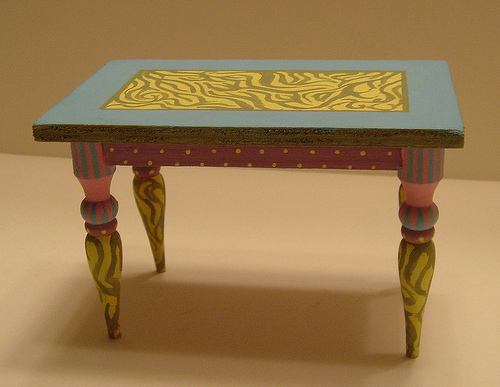
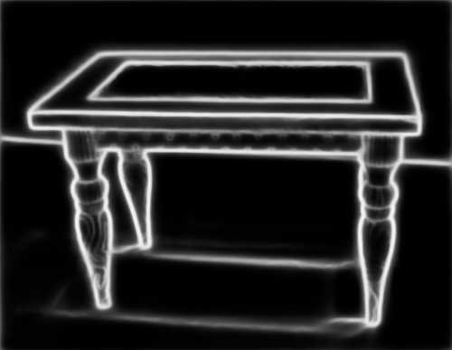
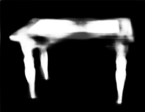
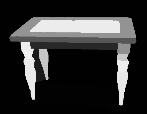
bottle
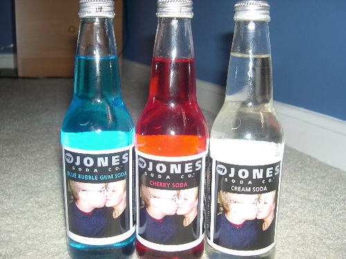
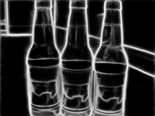
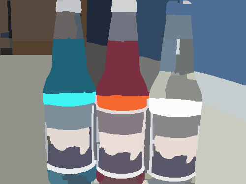
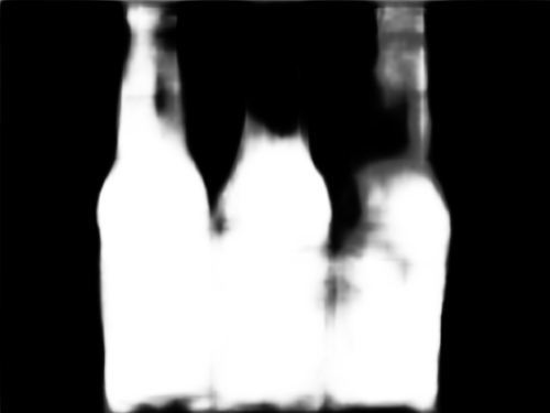
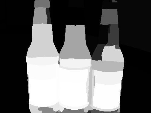
bicycle
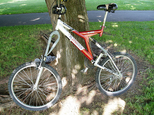
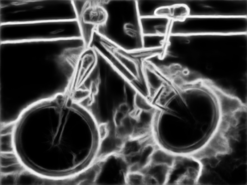
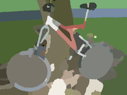
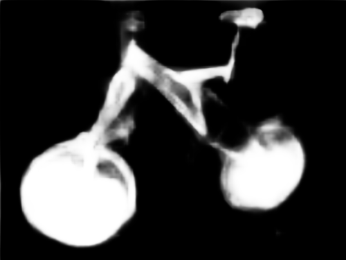
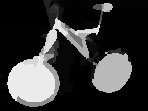
	(a) images	(b) edges	(c) regions	(d) saliency	(e) proxy GT

Figure 1: (a) Flickr images which are part of the result of searching on a keyword; (b) Edge maps produced by the RCF edge detector [18]; (c) Over-segmentation regions derived from (b) using the MCG method [19]; (d) Saliency maps generated by the DSS saliency detector [20]; (e) Proxy ground truths that can be directly computed by averaging the saliency values for each region. All the low-level cues can be used for any category without further training or finetuning.

We, as humans, are experts at quickly learning how to identify object regions by browsing example images searched using the corresponding keywords. Identifying object regions/boundaries and salient object regions of unknown categories easily helps us obtain enough pixel-wise ‘proxy ground truth’ annotations. Motivated by this phenomenon, this paper addresses the following question: could a machine vision system automatically learn semantic segmentation of unseen categories from web images that are the result of search keyword, without relying on any explicit user annotations? Very recently, some works, such as [21, 15, 13], have proposed various web-based learners attempting to solve the semantic segmentation problem. These methods indeed leverage web-crawled images/videos. However, they assume that each image/frame is associated with correct labels instead of considering how to solve the problem of label noise presenting in the web-crawled images/videos.

Our task vs. weakly supervised semantic segmentation. Conceptually, our task is quite different from traditional weakly supervised semantic segmentation as we must also deal with label noise. On one hand, in our task, only a set of target categories are provided rather than specific images with precise image-level annotations. This allows our task to be easily extended to cases where hundreds/thousands of target categories are given without collecting a large number of images with precise image-level labels. But this comes at a cost. Due to the typical diversity of web-crawled images, some of them may contain objects that are inconsistent with their corresponding query keywords (See Fig. 2). Therefore, how to deal with this label noise [22] becomes particularly important, which is one of our contributions.

As demonstrated in Fig. 1, we show some keyword-retrieved web images containing rich appearance varieties that can be used as training samples for semantic segmentation. With the help of low-level cues e.g., saliency, over-segmentation and edges, we are able to solve the semantic segmentation problem without relying on precise image-level noise free labels required by previous weakly supervised methods [12, 14, 10], which required attention cues [23]. For instance, edge information provides potential locations for object boundaries. Saliency maps tell us where the regions of interest are located. With these heuristics, the object regions that correspond to the query keywords become quite unambiguous for many images, making the unannotated web images a valuable source to be used as proxy ground truth for training semantic segmentation models. All the aforementioned low-level cues are category-agnostic, making automatically segmenting unseen categories possible.

Given the heuristic maps produced by imperfect heuristic generators, to overcome the noisy regions, previous weakly supervised semantic segmentation methods [12, 14, 24, 25, 13, 11] mostly harness image-level annotations (e.g. using PASCAL VOC dataset [1]) to correct wrong predictions for each heuristic map. In this paper, we consider this ticklish situation from a new perspective, which attempts to eliminate the negative effect caused by noisy proxy annotations. To do so, we propose to filter the irrelevant noisy regions by introducing an online noise filtering module. As a light weight branch, we embed it into a mature architecture (e.g., Deeplab [26]), to filter those regions with potentially wrong labels. We show that as long as the most regions are clean, by learning from the large amount of web data, we can still obtain good results.

To verify the effectiveness of our approach, we conduct extensive experiment comparisons on PASCAL VOC 2012 [1] dataset. Given 20 PASCAL VOC object category names, our WebSeg system retrieves 33,000 web images and immediately learn from these data without any manual assistant. The experimental results suggested that our WebSeg system, which does not use manually labeled image, is able to produce surprisingly good semantic segmentation results (mIOU = $\%57.0$). Our results are comparable with recently published state-of-the-art weakly supervised methods, which use tens of thousands of manually labeled images with precise keywords annotations. When additional keyword level weak supervision is provided, our WebSeg system could achieve an mIoU score of $\%63.3$, which significantly outperforms the existing weakly supervised semantic segmentation methods. We also carefully performed a serials of ablation studies to verify the importance of each component in our approach.

In summary, our contributions include:

• an attractive computer vision task, which aims at performing semantic segmentation by automatically learning from keyword-retrieved web images.

• an online noise filtering module (NFM), which is able to effectively filter potentially noisy region labels caused by the diversity of web-crawled images.

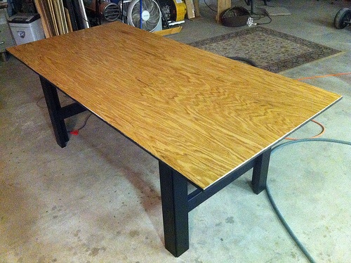
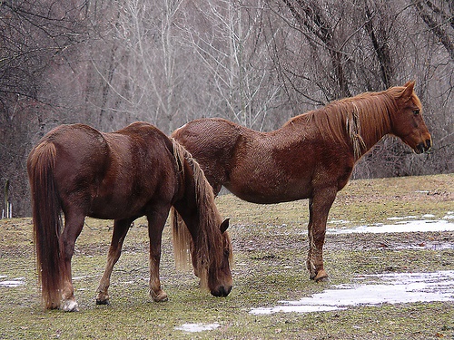
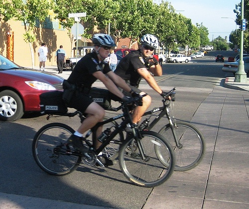
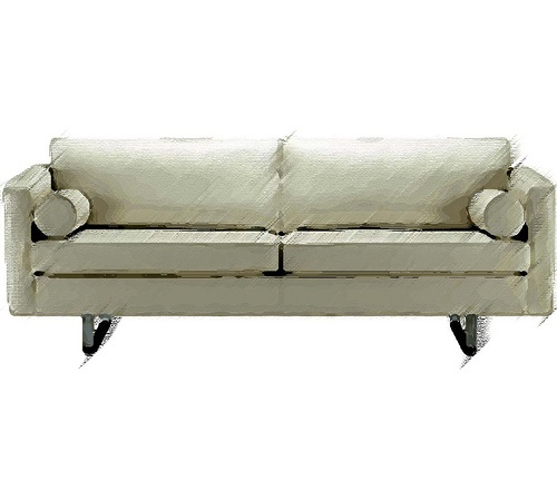
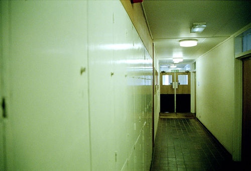
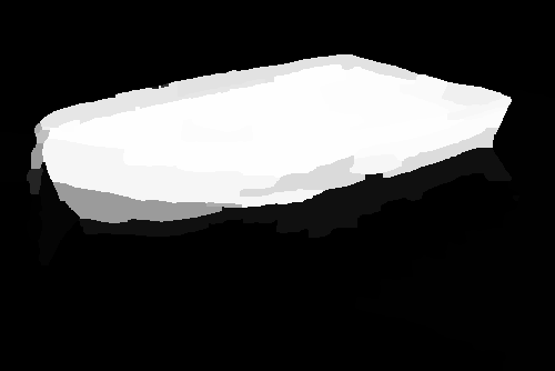
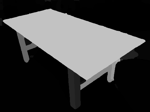
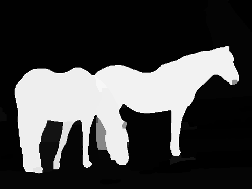
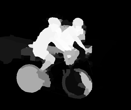
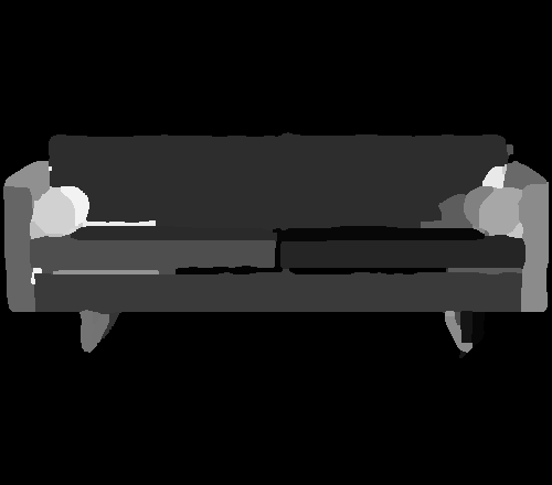
(a) boat	(b) table	(c) horse	(d) bicycle	(e) sofa	(f) potted plant

Figure 2: A group of images retrieved and the corresponding proxy ground truths. As can be seen, most of the semantic objects can be roughly segmented out despite a small number of failing samples.

2 Internet Images and Several Low-Level Cues

The cheapest way to obtain training images is to download them from the Internet (e.g., Flickr). Given a keyword or more, we are able to easily obtain a massive number of images that are very likely to be relevant, without reliable annotations at keyword or pixel level.

2.1 Crawling Training Images From the Internet

Given a collection of keyword, we first download 2,000 images for each category from the Flickr website according to relevance. Regarding the diversity of the fetched images, for example, some of them may have very complex background and some of them may also contain more than one semantic category (Fig. 2), we design a series of filtering strategies to automatically discard those images with low quality. To measure the complexity of the web images, we adopt the following schemes. First, we use the variance of the Laplacian [27, 28] to determine whether the input images are blurry. By convolving an image with the Laplace operator and computing the variance of the resulting map, we can obtain a score indicating how blurry the image is. In our experiment, we set a threshold 50 to throw away all the images that are larger than it. Second, we discard all the images with larger saturation and brightness values by transforming the input images from RGB color space to HSV space. This is reasonable as images with lower saturation and brightness are even difficult for humans to recognize. Specifically, we calculate the mean values of the H and V channels for each image. If either value is lower than 20, then the corresponding image will be abandoned. Finally, we get around 33,000 images for training.

2.2 Low-Level Cues

Web-crawled images do not naturally carry object region information with them. However, a three-year-old child could easily find precise object regions for most of these images, even if the corresponding object category has not been explicitly explained to him/her. This is mostly because of the capacity of humans processing low-level vision tasks. Inspired by this fact, we propose to leverage several low-level cues for the proposed task by mimicking the working mechanism of our vision system. In this paper, we take into account two types of low-level cues, including saliency and edge, which are also essential in our visual system when dealing with high-level vision tasks. Salient object detection models provide the locations of foreground objects as shown in Fig. 1(d) but weak knowledge on boundaries. As a remedy, edge detection models contain rich information about the boundaries, which can be used to improve the spatial coherence of our proxy ground truths. Specifically, for saliency detection, we use the DSS salient object detector [20] to generate saliency maps as done in [11]. For edge detection, we select RCF [18] as our edge detector which we found works better than the HED edge detector [29]. Furthermore, inspired by [30], we apply the MCG method [19] to the edge maps to get high-quality regions. Some visual results can be found in Fig. 1. As can be observed, with the help of edge information, some undetected salient regions can be segmented out. We will show some quantitative results when different heuristic cues are used in Sec. 4.

Formally, let $I$ denote an image with image labels $\mathbf{y}$, a subset of a predefined set $\mathcal{L}=\{l_{1},l_{2},\ldots,l_{L}\}$, where $L=|\mathcal{L}|$ denotes the number of semantic labels. We also use $l_{0}$ to denote the “background” category, so we have $\hat{\mathcal{L}}=\{l_{0},\mathcal{L}\}$. Further, let us denote $S$ and $R$ as the corresponding saliency and region maps of $I$, respectively. Then for each region $R_{m}\in R$, we perform the following snapping operation with respect to $S$

$$H_{j}=\frac{1}{|R_{m}|}\sum_{j\in R_{m}}S_{j},$$ (1)

where $H$ is the resulting heuristic map (i.e., the proxy ground truth annotation) used as supervision. Some visual results can be found in Fig. 1(e).

3 Online Noise Filtering

Due to the diversity of the downloaded images, it is very difficult to extract the desired information from them. This section is dedicated to presenting a promising mechanism to solve these problems, namely online noise filtering module (NFM).

3.1 Observations

Regarding the web-crawled images in our task, like weakly supervised semantic segmentation, one of the main issues is the noisy labels, which are from various weak cues. These low-level cues possibly contain parts of the semantic objects and even false predictions (Fig. 4), severely influencing the learning process of CNNs and leading to low-quality predictions. Furthermore, web-crawled images may contain more than one semantic category. For example, the images in the ‘bicycle’ category often cover the ‘person’ category and hence both of them will be predicted to salient regions with category ‘bicycle’ (Fig. 4a). Previous methods [10, 21] solved this problem using attention models [23]. However, the attention models themselves require the supervision of image-level labels that is impossible to be applied to our task. Regarding this challenge, a promising way to overcome this is to discard the noisy regions in the heuristic maps but meanwhile keep reliable ones unchanged. To achieve such a goal, in this section, we present an online noise filtering mechanism to intelligently filter those noisy regions.

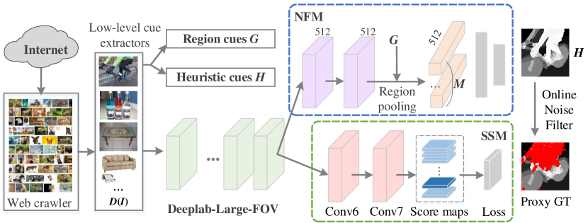
Figure 3: The overall architecture of the proposed method. The entire diagram can be separated into three main parts. The first one is a web crawler which is responsible for downloading Internet images given a collection of user-defined keywords. The second part extracts multiple different kinds of low-level cues and then combines them together as heuristics for learning. The last one is a semantic segmentation network with a noise filtering module (NFM). We use Deeplab-Large-FOV [26] as our baseline model in this paper.

Images
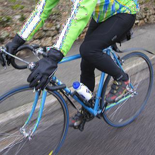
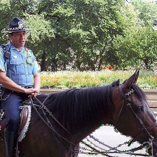
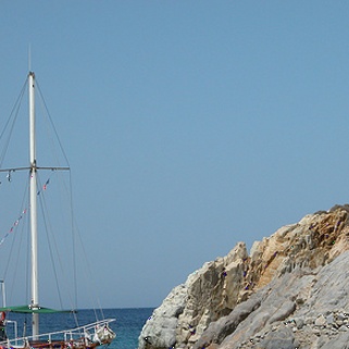
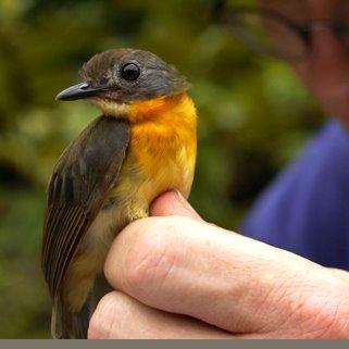
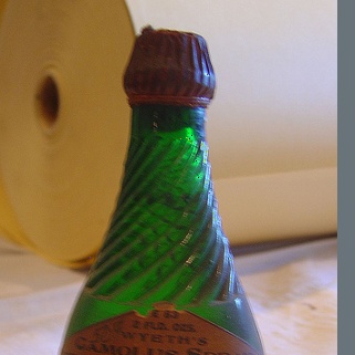
Heuristics
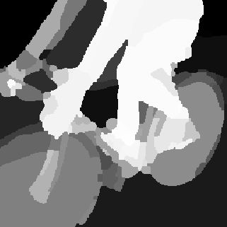
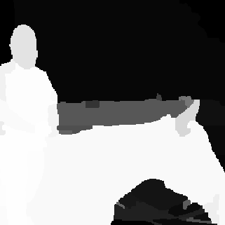
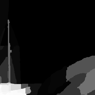
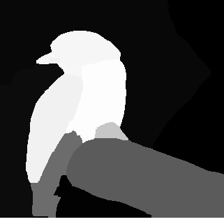
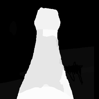
Results
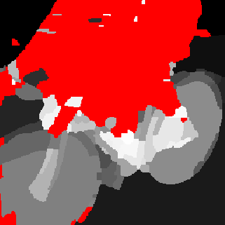
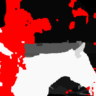
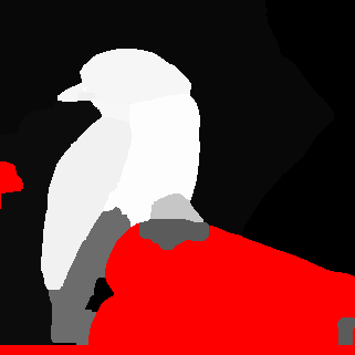
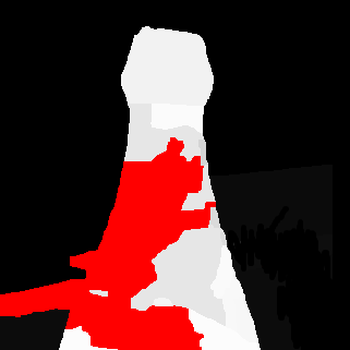
	(a) bicycle	(b) horse	(c) boat	(d) bird	(e) bottle

Figure 4: The results extracted from our NFM. Red regions are associated with special labels that will be ignored when optimizing SSM. (a-b) Ignoring irrelevant categories; (c-d) Ignoring undesired stuff from the heuristic maps.

Overview. The pipeline of our proposed approach can be found in Fig. 3. As the name implies, our proposed scheme is able to filter noisy labels online by introducing a noise filtering module (NFM) and then uses the generated heuristic maps as the supervision of the semantic segmentation module (SSM).

3.2 Online Noise Filtering

Noise Filtering Module (NFM). Given an image $I$ and its region map $R$, it is easy for us to predict the label of each region $R_{m}$. Specifically, the first part of our NFM consists of two convolutional layers for building higher-level feature representations, both of which have 512 channels, kernel size 3, and stride 1. Then, we introduce a channel-wise region pooling layer following the formulation of Eqn. (1) to extract equal number of features from each region. Suppose there were totally $M$ regions in image $I$, the dimensions of the output of the channel-wise region pooling layer would be $(M,512,1,1)$, i.e., the mini-batch is $M$. Finally, two fully connected layers are added as the classifier, which are with 1,024 and $|\mathcal{L}|$ neurons, respectively. Notice that all the weighted layers in our NFM are followed by ReLU layers for non-linear transformation apart from the last one. Please note that designing more complex structure might be more powerful here but this is beyond the scope of this paper as our goal is to show how to learn to discard those regions with potentially noisy labels.

Learning to Filter Noisy Labels. Given an image $I$ with image-level label $\mathbf{y}$ and its corresponding region map $R$ and heuristic map $H$, for any region $R_{m}$, if $\sum_{j\in R_{m}}{H_{j}}>0$ then we say that region $R_{m}$ belongs to foreground (otherwise background). During training, the ground truth label of each foreground region should be $\mathbf{y}$. For background regions, we give them a special label $l_{s}(l_{s}\notin\hat{\mathcal{L}})$, indicating that these regions should be ignored during training as we only care about foreground in NFM. Let us denote $f^{m}(I)$ as the activations corresponding to $R_{m}$ in the score layer of NFM. Notice that we omit the network parameters here for notational convenience. The predicted label of $R_{m}$ can be obtained by $C_{m}=\operatorname*{argmax}_{l\in\mathcal{L}}{f^{m}_{l}(I)}$. If $C_{m}\notin\mathbf{y}$, then $H_{j,j\in R_{m}}=l_{s}$. The resulting $H$ will be used as the annotation of SSM. The bottom row in Fig. 4 shows some typical examples of $H$. Compared to the middle row in Fig. 4, we can observe that our online noise filtering module indeed helps a lot when dealing with images with interferential categories.

Semantic Segmentation Module (SSM). The proxy annotations sent to SSM are gray-level continuous maps, each pixel of which indicates the probability of being foreground. Therefore, following [13], we use the following cross-entropy loss to optimize our SSM

$$\mathcal{E}(\theta)=\sum_{n=1}^{N}\left(\hat{p}_{n}^{0}\log p_{n}(l_{0}|I;\theta)+\hat{p}_{n}^{c}\log p_{n}(\mathbf{y}|I;\theta)\right),$$ (2)

where $N$ is the number of elements in $I$, $\theta$ is the network parameters, $\hat{p}_{n}^{c}=H_{n}$, denoting the probability of the $n$th element being salient, $\hat{p}_{n}^{0}=1-\hat{p}_{n}^{c}$, and $p_{n}(\mathbf{y}|I;\theta)$ the probability of the $n$th element belonging to $\mathbf{y}$, which is from the network prediction scores.

Training. During the training phase, we found that the NFM module always tends to over-fit when it reaches convergence. The classifier will predict the same label to almost all the foreground regions influenced by the noisy labels, which weakens the role of our NFM. To address this problem, we change the learning rate of the weighted layers in NFM by multiplying a fixed factor 0.1 to convolutional layers and 0.01 to fully connected layers. We empirically found that such an under-fitting state of NFM makes our whole model work the best. During the inference phase, we discard NFM while only keep the original layers in Deeplab. Therefore, we do not introduce any additional computation into the testing phase of Deeplab model.

3.3 Refinement

Input : Image $I$ from the training set; Image labels $\mathbf{y}$; Prediction scores $g(I)$

Output : $T$

1 for each pixel $j\in I$ do

2       $\hat{g}(j)\leftarrow\sigma(g(j))$, $\sigma$ is the softmax function ;

3       $\hat{T}(j)\leftarrow\frac{1}{Z(j)}\hat{g}(j)\cdot\mathbf{y}$, $Z(j)$ is the partition function;

4      

5 end for

6$\tilde{T}\leftarrow\text{CRF}(\hat{T})$ ;

7 $T\leftarrow\operatorname*{argmax}_{l\in\mathbf{y}}{\tilde{T}_{l}}$ ;

8

Algorithm 1 Generating “ground truth” for Refinement Stage

With the above CNN trained based on heuristic maps, it is possible for us to iteratively train more powerful CNNs by leveraging the supervision from the keywords as done in [13, 11]. Suppose in the $r$-th iteration of the learning process the network parameter is denoted by $\theta^{r}$. We can use $\theta^{r}$ to generate the prediction scores $g^{r}(I)$ of SSM. Given an image $I$, let $\mathbf{y}$ be its image-level labels. The segmentation map $T^{r}$ of $I$ can be computed according to Alg. 1. With $T^{r}$, we are able to optimize another CNN (the Deeplab model here), which may give us better results. Notice that after the first-round iteration, we do not use the NFM here any more as $T^{r}$ already provides us more reliable ‘ground truth.’ By carrying out the above procedures iteratively, we can gradually refine the segmentation results.

4 Experiments

Our autonomous web learning of the semantic segmentation task is similar to previous weakly supervised semantic segmentation task but now we can deal with label noise. To better verify the effectiveness of our proposed method, in this section, we compare our proposed approach with existing weakly supervised semantic segmentation methods and meanwhile analyze the importance of each component in our approach by ablation experiments. Differently from our new task which leverages only category-independent cues, traditional weakly supervised semantic segmentation methods also considers the knowledge of precise image-level labels (e.g., attention cues). For fair comparisons, we separate our experiments into two groups, which respectively represent weakly supervised semantic segmentation (including attention cues) and semantic segmentation with only category-independent cues.

4.1 Implementation Details

Datasets. In our experiment, we only use one keyword for each search. We denote the collected dataset with only web images as $\mathcal{D}(W)$, thus each image in $\mathcal{D}(W)$ is supposed to have only one semantic category. Furthermore, to compare our approach with existing weakly supervised methods, we choose the same datasets as in [11], which contain two parts. The first dataset is similar to our $\mathcal{D}(W)$, containing images with only single image-level labels, which are originally from the ImageNet dataset [31]. Here, we denote it as $\mathcal{D}(S)$. The second part, denoted as $\mathcal{D}(C)$, has only images from the PASCAL VOC 2012 benchmark [1] plus its augmented set [32]. More details can be found in Table 1. We evaluate our approach on the PASCAL VOC 2012 benchmark and report the results on both the ’val’ and ’test’ sets.

Low-Level Cues. Other than saliency cues and region cues, it is reasonable to harness attention cues [33] for weakly supervised semantic segmentation. Let us denote $A$ as the attention cues of image $I$. We first perform a pixel-wise maximum operation between $A$ and $S$ (saliency cues) as in [11], which aims to preserve as many heuristic cues as possible. Then, we use Eqn. 1 to perform a snapping operation with respect to the combined map, yielding the heuristic cues for training our first-round CNN.

Model Settings and Hyper-Parameters. We use the publicly available Caffe toolbox [34] as our implementation tool. Like most previous weakly supervised semantic segmentation works, we use VGGNet [35] as our pre-trained model. The hyper-parameters we used in this paper are as follows: initial learning rate (1e-3), divided by a factor of 10 after 10 epochs, weight decay (5e-4), momentum (0.9), and mini-batch size (16 for the first-round CNN and 10 for the second-round CNN). We train each model for 15 epochs. We also use the conditional random field (CRF) model proposed in [8] as a post-processing tool to enhance the spacial coherence, in which the graphical model is built upon regions. This is because we already have high-quality region cues which are derived from edge knowledge. Instead of both color and texture histograms as in [8], we only use the color histograms for measuring the similarities between adjacent regions as our regions are derived from edge maps which already contain semantic information. All the other settings are the same to [8].

Table 1: Dataset details and default dataset settings in each iteration. As WebSeg relies on only category-agnostic cues, the training images from PASCAL VOC dataset cannot be used. Because of space limitation, we use ‘weak’ to represent weakly supervised setting.

Datasets	#Images	single label	precise label	source	task
$\mathcal{D}(S)$	24,000	✓	✓	ImageNet [31]	weak (rounds 1 & 2 )
$\mathcal{D}(C)$	10,582	✗	✓	PASCAL VOC 2012 [1]	weak (round 2)
$\mathcal{D}(W)$	33,000	✓	✗	pure web	WebSeg (rounds 1 & 2)

Table 2: Ablations for our proposed approach. Notice that all the results are directly from our CNNs without using any post-processing tools unless noticed. The best result in each case are highlighted in bold. Inferior numerals represent the growth to the base numbers. All the results are measured on the PASCAL VOC 2012 validation set.

	First round IoU (%)
Low-Level Cues	Weak	WebSeg
sal	$52.59$	$49.92$
sal + edge	$54.39_{+1.80}$	$\mathbf{52.09_{+2.17}}$
sal + att + edge	$\mathbf{56.08_{+3.49}}$	—

(a) Low-level cues: Results when different low-level cues are used during the first-round iteration. For space convenience, we use the abbreviations of the cue names if needed. As can be seen, more low-level cues do help in both tasks.

NFM?	Region	Weak IoU (%)	WebSeg IoU (%)
✗	-	$56.08$	52.09
✓	Large	$56.46_{+0.38}$	-
✓	Medium	$56.54_{+0.46}$	-
✓	Small	$\mathbf{57.00_{+0.92}}$	$\mathbf{53.89_{+1.80}}$

(b) The role of our NFM: We use “Small”, “Medium”, and “Large” to represent the different sizes of regions derived from edges [18] by MCG [19]. Our NFM is especially useful when dealing with more noisy proxy ground truths (the right column).

4.2 Sensitivity Analysis

To analyze the importance of each component of our approach, we perform a number of ablation experiments in this subsection.

Low-Level Cues. The proposed learning paradigm starts with learning simple images and then transitions to general scenes following [13]. In this paragraph, we analyze the roles of different low-level cues and their combinations in the first-round iteration. For fair comparisons, we discard the NFM here whereas only keep the SSM. Table 2(a) shows the quantitative results of using different low-level cues. With only saliency cues, our first-round CNN achieves a baseline result with a mean IoU score of 52.59%. With the edge information incorporated, the baseline result can be improved by 1.8% in terms of mean IoU. When all three kinds of low-level cues are considered, we achieve the best results, which is 56.08%, around 3.5% improvement compared to the baseline result. Similar phenomenon can also be found when only utilizing web images in Table 2(a). These results verify the effectiveness of the low-level cues we leverage. By comparing the results on the two tasks in Table 2(a), we can observe that under the same experiment setting the web-crawled images are more complex than the images from the ImageNet. This is reasonable because unlike the ImageNet images the web-crawled images are not with accurate labels (See Fig. 2).

The Role of NFM. Table 2(b) lists the results when the NFM is used or not during the phase of training the first-round CNN. One can observe that with small regions provided, using NFM gives a 0.92% improvement compared to not using it and a 0.38% improvement compared to using large regions. Actually, the most important difference between whether using NFM lies in the ability of predicting images with multiple categories. As shown in Fig. 5 (columns c and d), our NFM is able to erase those noisy regions caused by the wrong predictions of saliency model and hence produces cleaner results. This phenomenon is especially obvious when training on web images. As shown in Table 2(b), there is an improvement of 1.8% on the ’val’ set during the first-round iteration compared to the baseline result without NFM. Compared to the growth range (+0.92%) with weak supervision, we can observe the noise-erasing ability of our NFM is essential, especially when handling noisy web images. From a visual standpoint, Fig. 4 provides more intuitive and direct results. Comparing the bottom two lines of Fig. 4, we can observe that our method after NFM successfully filters most noisy regions (undesired categories and stuffs in the background) in the heuristic cues. This makes our segmentation network learn cleaner knowledge from the heuristic cues.

Region Size in NFM. The region sizes play an important role in our NFM. Here, we compare the results when using different region sizes in our NFM. The regions are directly derived from the edge maps [18]. By building the Ultrametric Contour Maps (UCMs) [19] with different thresholds, we are allowed to obtain regions with different scales. Here, we show the results when setting threshold to 0, 0.25, and 0.75, which correspond to small, medium, and large regions, respectively. The quantitative results can be found in Table 2(b). As the number of regions increases, our approach achieves higher and higher mean IoU scores on the PASCAL VOC 2012 validation set. Training with small regions enables $0.54$ percent improvement compared to using large regions. The reason for this might be that lower thresholds provide more accurate regions, making less regions stretch over more than one category.

Table 3: Results based on different training set: As can be seen, our approach trained on only simple images has already achieved an IoU score of 58.79% for weakly supervised semantic segmentation. With the VOC training set incorporated, an IoU score of 60.45% can be obtained without using any post-processing tools, which is already better than most of the existing methods (See Table 5). When using images crawled from the Internet, we can also achieve a score of 54.78%.

Weakly		WebSeg
Train Set & #Images	IoU (%)	Train Set & #Images	IoU (%)
$\mathcal{D}(S)$,  24,000	$58.79$	$\mathcal{D}(W)$, 33,000	54.78
$\mathcal{D}(C)$,  10,582	$59.03_{+0.24}$	$\mathcal{D}(C)$, 10,582	—
$\mathcal{D}(S+C)$, 34,582	$\mathbf{60.45_{+1.66}}$	$\mathcal{D}(W+C)$, 43,582	$\mathbf{57.39_{+2.61}}$

Table 4: Results w/ and w/o CRF model: It is obvious that the CRF model greatly improves the results on both weakly supervised setting and WebSeg.

	First Round IoU (%)		Second Round IoU (%)
CRF Method	Weakly	WebSeg	Weakly	WebSeg
✗	$57.00$	$53.89$	60.45	54.78
CRF	$\mathbf{60.56_{+3.56}}$	$\mathbf{56.58_{+2.69}}$	$\mathbf{63.14_{+2.69}}$	$\mathbf{57.10_{+2.32}}$

The Role of CRF models. Conditional random filed models have been widely used in semantic segmentation tasks. In Table 4, we show the results when the CRF is used or not. Obviously, the CRF model does help in all cases.

The Role of Different Training Sets. We try to use different training sets to train the second-round CNN while keep all the setting of the first-round one unchanged. As can be seen in Table 3, combining both $\mathcal{D}(S)$ and $\mathcal{D}(C)$ allows us to obtain the best results, which is 1.66 points higher than only using $\mathcal{D}(S)$ for training. For pure web supervision, incorporating the images of $\mathcal{D}(C)$ is also helpful, which leads to a 2.61-point extra performance gain. This indicates that more high-quality training data does help and complex images provide more information between different categories that would be useful for both weakly supervised semantic segmentation and semantic segmentation with only web supervision.

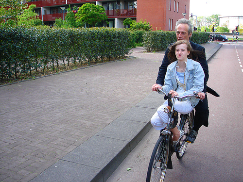
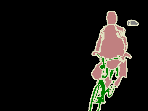
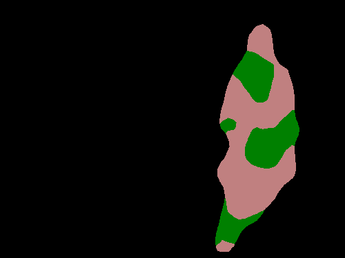
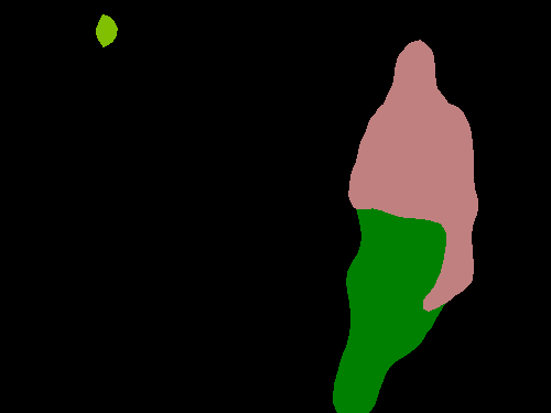
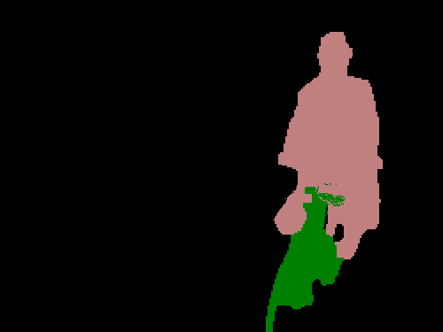
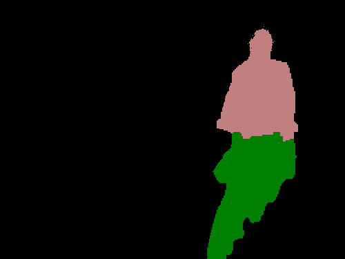
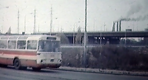
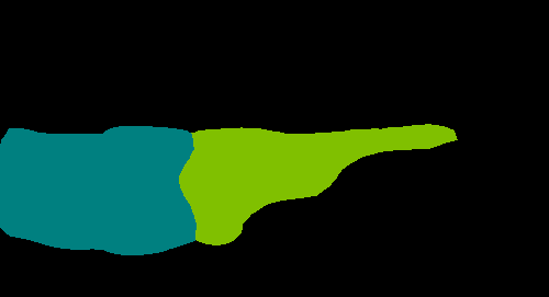
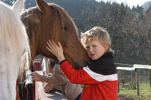
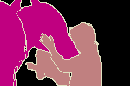
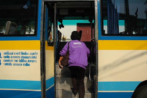
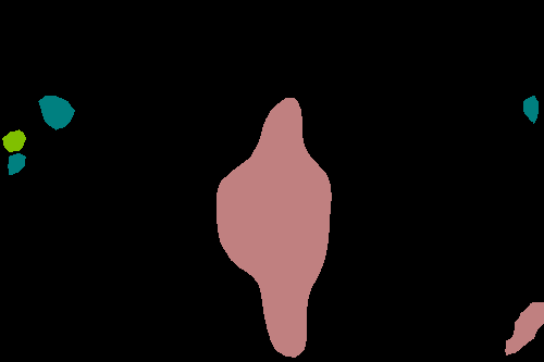
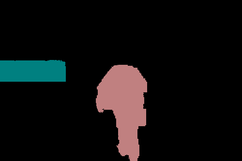
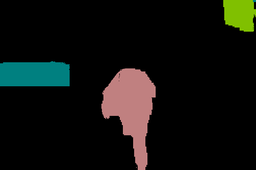
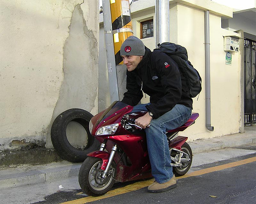
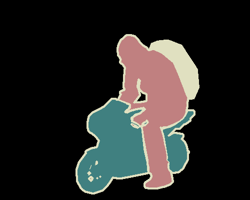
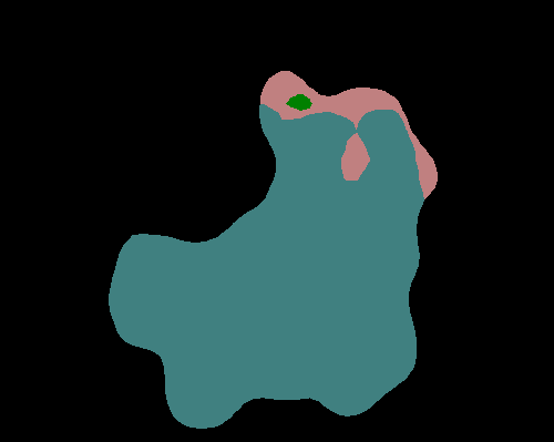
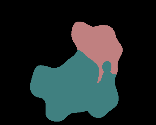
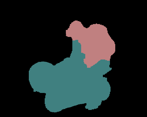
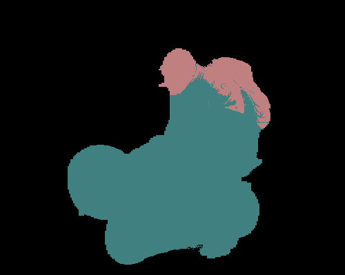
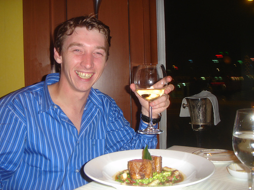
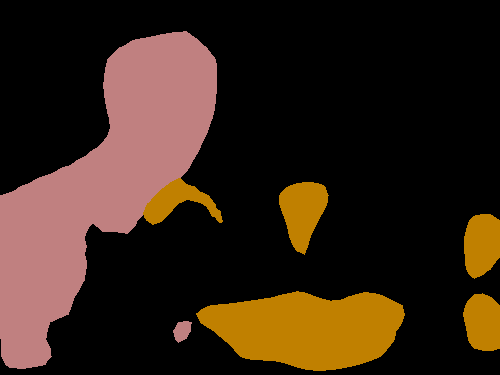
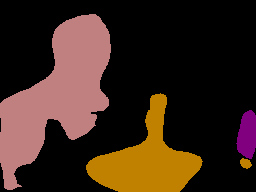
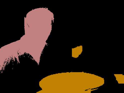
Source	GT	1st round w/o NFM	1st round w/ NFM	1st round + CRF	2nd round + CRF
(a)	(b)	(c)	(d)	(e)	(f)

Figure 5: Visual comparisons for weakly-supervised semantic segmentation using different settings of our proposed method. All the images come from the validation set of PASCAL VOC 2012 segmentation benchmark. Other than showing only successful results (the top 3 rows), we also show failure cases of our method (the bottom 3 rows).

4.3 Comparisons with Existing Works

In this subsection, we compare our approach with the existing state-of-the-art weakly supervised semantic segmentation works. All the methods compared here are based on the Deeplab-Large-FOV baseline model [26] except special declarations.

Table 5 lists the results of prior methods and ours on both ‘val’ and ‘test’ sets. As can be found, with weak supervision, our approach achieves a mean IoU score of $60.5\%$ on the ‘val’ set without using CRF. This value is already far better than the results of all prior works no matter whether the CRFs are used for them. By using CRFs as post-processing tools, our method realizes the best results on the ‘val’ and ‘test’ sets, which are both higher than 63.0%. When considering training on web images with only category-agnostic cues, our results on both the ‘val’ and ‘test’ sets are also better than most previous works and comparable to the state-of-the-arts. This reflects that despite extremely noisy web images, our approach is robust as well. This is mostly due to the effectiveness of our proposed architecture, the ability of eliminating the effect of noisy heuristic cues.

Table 5: Quantitative comparisons with the existing state-of-the-art approaches on both ‘val’ and ‘test’ sets. The best result in each column is highlighted in Bold. For fair comparisons, we split the table into two parts according to the type of supervision. We also abbreviation ‘weak’ to denote weakly supervised approaches and ‘web’ the approach with web supervision. ‘$\dagger$’ stands for our results with weak supervision.

Methods	Supervision		mIoU (val)		mIoU (test)
	weak	web	w/o CRF	w/ CRF	w/ CRF
CCNN [36], ICCV’15	✓		33.3%	35.3%	-
EM-Adapt [6], ICCV’15	✓		-	38.2%	39.6%
MIL [37], CVPR’15	✓		42.0%	-	-
SEC [12], ECCV’16	✓		44.3%	50.7%	51.7%
AugFeed [7], ECCV’16	✓		50.4%	54.3%	55.5%
STC [13], PAMI’16	✓		-	49.8%	51.2%
Roy et al. [38], CVPR’17	✓		-	52.8%	53.7%
Oh et al. [39], CVPR’17	✓		51.2%	55.7%	56.7%
AS-PSL [14], CVPR’17	✓		-	55.0%	55.7%
Hong et al. [21], CVPR’17	✓		-	58.1%	58.7%
WebS-i2 [15], CVPR’17	✓		-	53.4%	55.3%
DCSP-VGG16 [10], BMVC’17	✓		56.5%	58.6%	59.2%
Mining Pixels [11], EMMCVPR’17	✓		56.9%	58.7%	59.6%
$\text{WebSeg}^{\dagger}~{}\text{(Ours)}$	✓		60.5%	63.1%	63.3%
WebSeg (Ours)		✓	54.78%	57.10%	57.04%

4.4 Discussion

In Table 6, we show the specific number of each category on both the ‘val’ and ‘test’ sets . As can be observed, with the supervision of accurate image-level labels, our approach wins the other existing methods on most categories (the purple line). However, there are also some unsatisfactory results for a few categories (e.g., ‘chair’ and ‘table’). This small set of categories are normally with strange shapes and hence difficult to be detected by current low-level cues extractors. For instance, our method on the ‘table’ category gets a IoU score of 24.1%, which is nearly 8% worse than the AS-PSL method [14]. This is mainly due to the fact that AS-PSL mostly relies on the attention cues, which performs better on detecting the location of semantic objects.

Regarding the results with web supervision, in spite of only several low-level cues and extremely noisy web images, our approach can get comparable results to the best weakly supervised methods. More interestingly, our approach behaves the best on two categories on the ‘test’ set (‘bicycle’ and ‘train’). This implies that leveraging reliable low-level cues provides a promising way to deal with learning semantic segmentation automatically from the Internet.

Failure Case Analysis. Besides the successful samples, there are also many failure cases that have been exhibited on the bottom part of Fig. 5. One of the main reasons leading to this should be the wrong predictions of the heuristic cues. Although our online noise filtering mechanism, to some extent, is able to eliminate the interference brought by noises, it still fails when processing some very complicated scenes. For example, in Fig. 4a, it is very hard to distinguish clearly which regions belong to ‘bicycle’ and which regions belong to ‘person.’ On the other hand, the simple images cannot incorporate all the scenes in the ‘test’ set and therefore results in many semantic regions undetected.

Table 6: Quantitative result comparisons with previous methods on each category. All the methods listed here are recent state-of-the-art methods. ‘${\dagger}$’ means our methods with weak supervision. The best result in this column has been highlighted in bold. It can easily found that our approach based on weakly supervised setting works better than all the other methods on most categories.

Methods	bkg	plane	bike	bird	boat	bottle	bus	car	cat	chair	cow	table	dog	horse	motor	person	plant	sheep	sofa	train	tv	mean
STC	84.5	68.0	19.5	60.5	42.5	44.8	68.4	64.0	64.8	14.5	52.0	22.8	58.0	55.3	57.8	60.5	40.6	56.7	23.0	57.1	31.2	49.8
Roy et al.	85.8	65.2	29.4	63.8	31.2	37.2	69.6	64.3	76.2	21.4	56.3	29.8	68.2	60.6	66.2	55.8	30.8	66.1	34.9	48.8	47.1	52.8
AS-PSL	83.4	71.1	30.5	72.9	41.6	55.9	63.1	60.2	74.0	18.0	66.5	32.4	71.7	56.3	64.8	52.4	37.4	69.1	31.4	58.9	43.9	55.0
WebS-i2	84.3	65.3	27.4	65.4	53.9	46.3	70.1	69.8	79.4	13.8	61.1	17.4	73.8	58.1	57.8	56.2	35.7	66.5	22.0	50.1	46.2	53.4
Hong et al.	87.0	69.3	32.2	70.2	31.2	58.4	73.6	68.5	76.5	26.8	63.8	29.1	73.5	69.5	66.5	70.4	46.8	72.1	27.3	57.4	50.2	58.1
MiningP	88.6	76.1	30.0	71.1	62.0	58.0	79.2	70.5	72.6	18.1	65.8	22.3	68.4	63.5	64.7	60.0	41.5	71.7	29.0	72.5	47.3	58.7
$\textbf{WebSeg}^{\dagger}$	89.6	85.6	32.3	76.1	68.3	68.7	84.2	74.9	78.2	18.6	75.0	24.1	75.2	69.9	67.0	63.9	40.8	77.9	32.8	69.7	53.3	63.1
WebSeg	88.6	81.6	32.9	75.7	57.6	57.7	79.5	69.2	74.4	12.6	71.7	12.3	73.2	66.5	61.6	58.6	21.1	73.9	25.1	69.9	35.3	57.1
STC	85.2	62.7	21.1	58.0	31.4	55.0	68.8	63.9	63.7	14.2	57.6	28.3	63.0	59.8	67.6	61.7	42.9	61.0	23.2	52.4	33.1	51.2
Roy et al.	85.7	58.8	30.5	67.6	24.7	44.7	74.8	61.8	73.7	22.9	57.4	27.5	71.3	64.8	72.4	57.3	37.0	60.4	42.8	42.2	50.6	53.7
AS-PSL	-	-	-	-	-	-	-	-	-	-	-	-	-	-	-	-	-	-	-	-	-	55.7
WebS-i2	85.8	66.1	30.0	64.1	47.9	58.6	70.7	68.5	75.2	11.3	62.6	19.0	75.6	67.2	72.8	61.4	44.7	71.5	23.1	42.3	43.6	55.3
Hong et al.	87.2	63.9	32.8	72.4	26.7	64.0	72.1	70.5	77.8	23.9	63.6	32.1	77.2	75.3	76.2	71.5	45.0	68.8	35.5	46.2	49.3	58.7
MiningP	88.9	72.7	31.0	76.3	47.7	59.2	74.3	73.2	71.7	19.9	67.1	34.0	70.3	66.6	74.4	60.2	48.1	73.1	27.8	66.9	47.9	59.6
$\textbf{WebSeg}^{\dagger}$	89.8	78.6	32.4	82.9	52.9	61.5	79.8	77.0	76.8	18.8	75.7	34.1	75.3	75.9	77.1	65.7	46.1	78.9	32.3	65.3	52.8	63.3
WebSeg	88.6	74.7	33.3	74.8	49.2	62.1	75.4	75.5	71.8	16.0	65.6	15.6	71.2	68.9	72.1	58.6	24.7	72.8	19.1	67.5	40.3	57.0

5 Conclusion and Discussion

In this paper, we propose an interesting but challenging computer vision problem, namely WebSeg, which aims at learning semantic segmentation from the free web images following the learning manner of humans. Regarding the extremely noisy web images and their imperfect proxy ground-truth annotations, we design a novel online noise filtering mechanism, a new learning paradigm, to let CNNs know how to discard undesired noisy regions. Experiments show that our learning paradigm with only training on web images has already obtained comparable results compared to previous state-of-the-art methods. When leveraging more weak cues as in weakly supervised semantic segmentation, we further improve the results by a large margin. Moreover, we also perform a series of ablation experiments to show how each component in our approach works.

Despite this, there is still a large room for improving the results of our task, which is based on purely web supervision. According to Table 6, the mIoU scores of a few categories are still low. Thereby, how to download good web images, improve the quality of heuristic cues, and design useful noise-filtering mechanisms are interesting future directions. This new topic, as mentioned above, covers a series of interesting but difficult techniques, offering many valuable research directions which need to be further delved into. In summary, automatically learning knowledge from the unrestricted Internet resources substantially reduce the intervention of humans. We hope such a interesting vision task could drive the rapid development of its relevant research topics as well.

References

- [1] Everingham, M., Eslami, S.A., Van Gool, L., Williams, C.K., Winn, J., Zisserman, A.: The pascal visual object classes challenge: A retrospective. IJCV (2015)
- [2] Cordts, M., Omran, M., Ramos, S., Rehfeld, T., Enzweiler, M., Benenson, R., Franke, U., Roth, S., Schiele, B.: The cityscapes dataset for semantic urban scene understanding. In: CVPR. (2016) 3213–3223
- [3] Zhao, H., Shi, J., Qi, X., Wang, X., Jia, J.: Pyramid scene parsing network. In: CVPR. (2017)
- [4] Lin, G., Milan, A., Shen, C., Reid, I.: Refinenet: Multi-path refinement networks with identity mappings for high-resolution semantic segmentation. In: CVPR. (2017)
- [5] Lin, G., Shen, C., van den Hengel, A., Reid, I.: Efficient piecewise training of deep structured models for semantic segmentation. In: CVPR. (2016)
- [6] Papandreou, G., Chen, L.C., Murphy, K., Yuille, A.L.: Weakly-and semi-supervised learning of a dcnn for semantic image segmentation. In: ICCV. (2015)
- [7] Qi, X., Liu, Z., Shi, J., Zhao, H., Jia, J.: Augmented feedback in semantic segmentation under image level supervision. In: ECCV. (2016)
- [8] Lin, D., Dai, J., Jia, J., He, K., Sun, J.: Scribblesup: Scribble-supervised convolutional networks for semantic segmentation. In: CVPR. (2016)
- [9] Bearman, A., Russakovsky, O., Ferrari, V., Fei-Fei, L.: What’s the point: Semantic segmentation with point supervision. In: ECCV. (2016) 549–565
- [10] Chaudhry, A., Dokania, P.K., Torr, P.H.: Discovering class-specific pixels for weakly-supervised semantic segmentation. BMVC (2017)
- [11] Hou, Q., Dokania, P.K., Massiceti, D., Wei, Y., Cheng, M.M., Torr, P.: Bottom-up top-down cues for weakly-supervised semantic segmentation. EMMCVPR (2017)
- [12] Kolesnikov, A., Lampert, C.H.: Seed, expand and constrain: Three principles for weakly-supervised image segmentation. In: ECCV. (2016)
- [13] Wei, Y., Liang, X., Chen, Y., Shen, X., Cheng, M.M., Feng, J., Zhao, Y., Yan, S.: Stc: A simple to complex framework for weakly-supervised semantic segmentation. IEEE TPAMI (2016)
- [14] Wei, Y., Feng, J., Liang, X., Cheng, M.M., Zhao, Y., Yan, S.: Object region mining with adversarial erasing: A simple classification to semantic segmentation approach. In: CVPR. (2017)
- [15] Jin, B., Ortiz Segovia, M.V., Susstrunk, S.: Webly supervised semantic segmentation. In: CVPR. (2017) 3626–3635
- [16] Papadopoulos, D.P., Clarke, A.D., Keller, F., Ferrari, V.: Training object class detectors from eye tracking data. In: ECCV, Springer (2014) 361–376
- [17] Mitchell, T.M., Cohen, W.W., Hruschka Jr, E.R., Talukdar, P.P., Betteridge, J., Carlson, A., Mishra, B.D., Gardner, M., Kisiel, B., Krishnamurthy, J., et al.: Never ending learning. In: AAAI. (2015) 2302–2310
- [18] Liu, Y., Cheng, M.M., Hu, X., Wang, K., Bai, X.: Richer convolutional features for edge detection. In: CVPR. (2017)
- [19] Pont-Tuset, J., Arbelaez, P., Barron, J.T., Marques, F., Malik, J.: Multiscale combinatorial grouping for image segmentation and object proposal generation. IEEE TPAMI (2017)
- [20] Hou, Q., Cheng, M.M., Hu, X., Borji, A., Tu, Z., Torr, P.: Deeply supervised salient object detection with short connections. In: CVPR. (2017)
- [21] Hong, S., Yeo, D., Kwak, S., Lee, H., Han, B.: Weakly supervised semantic segmentation using web-crawled videos. In: CVPR. (2017) 3626–3635
- [22] Frénay, B., Kabán, A., et al.: A comprehensive introduction to label noise. In: ESANN. (2014)
- [23] Zhou, B., Khosla, A., Lapedriza, A., Oliva, A., Torralba, A.: Learning deep features for discriminative localization. In: CVPR. (2016)
- [24] Krähenbühl, P., Koltun, V.: Efficient inference in fully connected crfs with gaussian edge potentials. In: NIPS. (2011)
- [25] Zheng, S., Jayasumana, S., Romera-Paredes, B., Vineet, V., Su, Z., Du, D., Huang, C., Torr, P.H.: Conditional random fields as recurrent neural networks. In: ICCV. (2015)
- [26] Chen, L.C., Papandreou, G., Kokkinos, I., Murphy, K., Yuille, A.L.: Semantic image segmentation with deep convolutional nets and fully connected crfs. In: ICLR. (2015)
- [27] Pech-Pacheco, J.L., Cristóbal, G., Chamorro-Martinez, J., Fernández-Valdivia, J.: Diatom autofocusing in brightfield microscopy: a comparative study. In: ICPR. (2000)
- [28] Pertuz, S., Puig, D., Garcia, M.A.: Analysis of focus measure operators for shape-from-focus. Pattern Recognition (2013)
- [29] Xie, S., Tu, Z.: Holistically-nested edge detection. IJCV (2017)
- [30] Maninis, K.K., Pont-Tuset, J., Arbelaez, P., Van Gool, L.: Convolutional oriented boundaries: From image segmentation to high-level tasks. IEEE TPAMI (2017)
- [31] Russakovsky, O., Deng, J., Su, H., Krause, J., Satheesh, S., Ma, S., Huang, Z., Karpathy, A., Khosla, A., Bernstein, M., et al.: Imagenet large scale visual recognition challenge. IJCV (2015)
- [32] Hariharan, B., Arbeláez, P., Bourdev, L., Maji, S., Malik, J.: Semantic contours from inverse detectors. In: ICCV. (2011)
- [33] Zhang, J., Lin, Z., Brandt, J., Shen, X., Sclaroff, S.: Top-down neural attention by excitation backprop. In: ECCV. (2016)
- [34] Jia, Y., Shelhamer, E., Donahue, J., Karayev, S., Long, J., Girshick, R., Guadarrama, S., Darrell, T.: Caffe: Convolutional architecture for fast feature embedding. In: ACM Multimedia. (2014)
- [35] Simonyan, K., Zisserman, A.: Very deep convolutional networks for large-scale image recognition. In: ICLR. (2015)
- [36] Pathak, D., Krahenbuhl, P., Darrell, T.: Constrained convolutional neural networks for weakly supervised segmentation. In: ICCV. (2015)
- [37] Pinheiro, P.O., Collobert, R.: From image-level to pixel-level labeling with convolutional networks. In: CVPR. (2015)
- [38] Roy, A., Todorovic, S.: Combining bottom-up, top-down, and smoothness cues for weakly supervised image segmentation. In: CVPR. (2017)
- [39] Oh, S.J., Benenson, R., Khoreva, A., Akata, Z., Fritz, M., Schiele, B.: Exploiting saliency for object segmentation from image level labels. In: CVPR. (2017)