Three Birds One Stone: A General Architecture for Salient Object Segmentation, Edge Detection and Skeleton Extraction

Abstract

In this paper, we aim at solving pixel-wise binary problems, including salient object segmentation, skeleton extraction, and edge detection, by introducing a general architecture. Previous works have proposed tailored methods for solving each of the three tasks independently. Here, we show that these tasks share some similarities that can be exploited for developing a general architecture. In particular, we introduce a horizontal cascade of encoders so as to gradually advance the feature representations from the original CNN trunks. To better fuse feature at different levels, the inputs of each encoder in our architecture is densely connected to the outputs of its previous encoder. Stringing these encoders together allows us to effectively exploit features across different levels hierarchically to effectively address multiple pixel-wise binary regression tasks. To assess the performance of our proposed network on these tasks, we carry out exhaustive evaluations on multiple representative datasets. Although these tasks are inherently very different, we show that our approach performs very well on all of them and works far better than current single-purpose state-of-the-art methods. We also conduct sufficient ablation analysis to let readers better understand how to design encoders for different tasks. The source code in this paper will be publicly available after acceptance.

I Introduction

Convolutional neural networks (CNNs) have been widely used in most fundamental computer vision tasks (e.g., semantic segmentation [1, 2], edge detection [3], salient object segmentation [4, 5, 6, 7], skeleton extraction [8, 9].) and have achieved unprecedented performance on many tasks. To date, most of the existing methods are designed only for a single task because different tasks often favor different types of features. Their design criterion is single-purpose, greatly restricting their applicability to other tasks [10]. For example, the Holistically-nested Edge Detector (HED) [3] works well for the edge detection task but does not perform well for salient object detection [5] and skeleton extraction [11]. The reason is that the architecture proposed in HED does not consider how to capture homogeneous region information and scale-variant (either thick or thin) skeletons.

In this paper, our goal is to present a general architecture for solving three important binary problems, including salient object segmentation, edge detection, and skeleton extraction. As popular low-level vision tasks, all of them have been widely studied recently. In Fig. 1, we illustrate a 2D space representing features that these tasks favor. Specifically, salient object segmentation, as addressed in many existing works [4, 12, 5, 13, 14, 15], requires the ability to extract homogeneous regions and hence relies more on high-level features (Fig. 2c and 2f). Edge detection aims at detecting accurate boundaries, thus it needs more low-level features to sharpen the coarse edge maps produced by deeper layers [3, 16] (Fig. 2d and 2e). Skeleton extraction [8, 9], on the other hand, prefers high-level semantic information to detect scale-variant (either thick or thin) skeletons. From the standpoint of the network architecture, in spite of three different tasks, all of them require multi-level features in varying degrees (See Fig. 1). Consequently, a natural question is whether it is possible to combine multi-level features in a proper way such that stronger and more general feature representations can be constructed for solving all of these tasks.

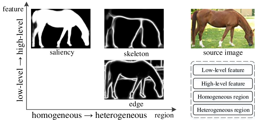
Figure 1: Preferred features of different tasks in our work. On the right side, we show the source image and two dimensions of features favored by different tasks. The results on the left side are all by our approach.

To solve the above question, rather than simply combining the multi-level features extracted from the trunk of CNNs as done in most existing works [5, 3, 11, 17], we propose to horizontally construct a cascade of encoders to gradually encode signals from the CNN trunks (Fig. 3a) to make the final representations more powerful. Each encoder is composed of multiple transition nodes, each of which gets input from its former encoder, enabling subsequent encoders to efficiently select features from the backbone in a dense manner. As the signals from the backbone pass through the encoders sequentially, more and more advanced feature representations can be built that can be applied to different tasks. As shown in Fig. 2, our approach is more general compared to existing relevant methods. To evaluate the performance of the proposed architecture, we apply it to three binary tasks— salient object detection, edge detection, and skeleton extraction. Experimental results show that our approach outperforms existing methods on multiple widely used benchmarks. Specifically, for salient object detection, compared to previous state-of-the-art works, our method has a performance gain of nearly 2% on average on 5 popular datasets. For skeleton extraction, we also significantly improve the state-of-the-art results by more than 2% in terms of F-measure. Furthermore, to let readers better understand the proposed approach, we conduct a series of ablation experiments for all three tasks.

To sum up, the contributions of this paper can be summarized as follows:

• First, we analyse the similarities as well as differences among salient object segmentation, edge detection, and skeleton extraction and design a general architecture to solve all these tasks;

• Second, we propose to construct a horizontal cascade of encoders to progressively extract more general feature representations that can be competent for all these tasks.

The rest of the paper is organized as follows. Section II reviews a number of recent works that are strongly related to our tasks and meanwhile analyzes the differences among different CNN-based skip-layer architectures. Section III presents the observations of this paper and describe the architecture of our proposed approach in detail. Section IV-VI compares the proposed approach with other state-of-the-art results and at the same time provide sufficient ablation analysis to let readers better understand how each component works in our architecture. Finally, Section VII concludes the whole paper and highlights some potential research directions.

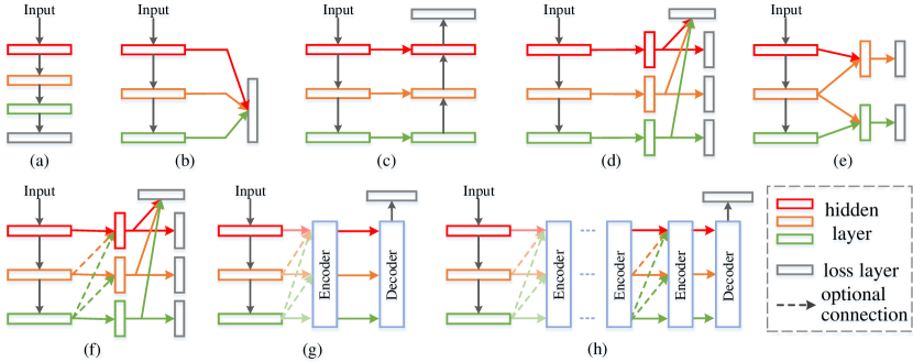
Figure 2: Architecture comparisons. (b) DCL [4]; (c) MSRNet [12]; (d) HED [3]; (e) COB [16]; (f) SRN [9] and DSS [5]; (g) Our architecture with one encoder; (h) A general case of our architecture. Note that many existing methods share the same architecture as one of the illustrations shown here. We only show the representative one for each structure.

II Related Works

In this section, we first review a number of popular methods that are strongly related to the tasks we solve and then analyze CNN-based skip-layer architectures that have been proposed recently.

II-A Salient Object Detection

Earlier salient object detection methods mostly rely on hand-crafted features, including either local contrast cues [18, 19, 20] or global contrast cues [21, 22, 23, 24, 25]. Interested readers may refer to some notable review and benchmark papers [26, 27, 28] for detailed descriptions. Apart from the classic methods, a number of deep learning based methods have recently emerged. In [29], He et al. presented a superpixel-wise convolutional neural network architectures to extract hierarchical contrast features for predicting the saliency value of each region. Li et al. [30] proposed to feed different levels of image segmentation into three CNN branches and aggregate the multi-scale output features to predict whether each region is salient. Wang et al. [31] considered both local and global information by designing two different networks. The first one is used to learn local patch features to provide each pixel a saliency value and then, multiple kinds of information are merged together as the input to the second network to predict the saliency score of each region. Similarly, in [32], Zhao et al. designed two different CNNs to independently capture the global and local context information of each segment patch, and then fed them into a regressor to output a saliency score for each patch.

The above methods took as input image patches and then used CNN features to predict the saliency of each input region (either a bounding box [33] or a superpixel [34, 35]). Later works, benefiting from the high efficiency of fully convolutional networks [1] (FCNs), utilize the strategy in which spatial information is processed in CNNs, and hence produce remarkable results. Lee et al. [36] combined both high-level semantic features extracted from CNNs and hand-crafted features and then utilized a unified fully-connected neural network to estimate saliency score of each query region. Liu et al. [37, 38] refine the details of the prediction maps progressively by harnessing recurrent fully convolutional networks. In [4], Li et al. combined a pixel-level fully convolutional stream and a segment-wise spatial pooling stream into one network to better leverage the contrast information of the input images. Hou et al. [5] and Li et al. [12] hierarchically fused multi-level features in a top-down manner. More recently, Zhang et al. [39] designed a generic architecture to aggregating multi-level CNN features. In [40], Zhang et al. embedded R-Dropout and hybrid upsampling layers into an encoder-decoder structure to better localize the salient objects.

II-B Edge Detection.

Early edge detection works [41, 42, 43] mostly relied on various gradient operators. Later works, such as [44, 45, 46], were driven by manually-designed features and were able to improve the performance compared to gradient-based works. Recently, with the emergence of large scale datasets, learning-based methods [47, 48, 49, 50] gradually became the main stream for edge detection. Further, recent CNN-based methods [51, 52, 53, 54, 3, 55, 16, 56] have started a new wave in edge detection research. Ganin et al. [51] proposed to use both CNN features and the nearest neighbour search to detect edges. In [52], the contour data was separated into different subclasses and different model parameters were learned for each subclass. Hwang [54] viewed edge detection as a per-pixel classification problem by learning a feature vector for each pixel.

Different from pixel/patch level analysis methods, Xie and Tu [3] designed a holistically-nested edge detector (HED) by introducing the concept of side supervision into a fully convolutional networks to merge features from different levels. In [55], multiple cues are considered to improve the precision of edges. Liu et al. [56] advanced the HED architecture by extracting richer convolutional features from CNNs.

II-C Skeleton Extraction.

Earlier methods [57, 58, 59] mainly relied on gradient intensity maps of natural images to extract skeletons. Later learning-based methods viewed skeleton extraction as a per-pixel classification problem. In [60], Tsogkas and Kokkinos calculated hand-crafted multi-scale and multi-orientation features for each pixel and utilized multiple instance learning to predict the score of each pixel. Sironi et al. [61] attempted to learn distance to the closest skeleton segment for each pixel. There are also some approaches [62, 63] computing the similarity between superpixels and combined them by clustering or filtering schemes.

Recent skeleton detection methods [8, 9] are mainly based on the holistically-nested edge detector (HED). In [8], Shen et al. introduced supervision in different blocks by guiding the scale-associated side outputs toward ground-truth skeletons at different scales and then fused multiple scale-associated side outputs in a scale-specific manner to localize skeleton pixels at multiple scales. Ke et al. [9] added multiple shortcuts from deeper blocks to shallower ones based on the HED architecture such that high-level semantic information can be effectively transmitted to lower side outputs, yielding stronger features.

II-D CNN-Based Skip-Layer Architectures

Unlike most classification tasks which adopt the classic bottom-up structures (Fig. 2a), region segmentation and edge detection tasks depend on how homogeneous regions are extracted and how edges are sharpened. Intuitively, considering the fact that lower network layers are capable of capturing local details while higher layers capture high-level contextual details, a good solution to satisfy the above needs might be introducing skip-layer architectures [1]. One of the recent successful CNN-based skip-layer structures is the HED architecture [3], which learns rich hierarchical features by means of adding side supervision to each side output (Fig. 2d). This architecture treats features at different levels equally, and therefore allows enough edge details to be captured through lower side outputs. Afterwards, several follow-up works [55, 8, 16, 56] adopted similar structures (e.g., by introducing deep supervision) to capture richer feature representations by fusing features at different levels.

There are also some other work modifying this structure by adding short connections [5, 9] from upper layers to lower ones to better leverage multi-level features for salient object detection and skeleton extraction or gradually refine the coarse-level features in a top-down manner [64, 65]. These approaches, however, only attempt to simply combine multi-level features. There is still a large room for extracting richer feature representations for these pixel-wise binary regression problems.

Figure 3: (a) A typical representation of our proposed general architecture. (b) Detailed illustration of a transition node in each middle encoder. Thin solid lines are required while thin dash ones are optional. Thick lines (horizontal signal flow and side path) are used for demonstration purpose only.

III The Proposed General Architecture

In this section, we elaborate on the similar characteristics shared by salient object detection, skeleton extraction, and edge detection tasks and propose a general architecture that can treat them all.

III-A Key Observations

Previous works leverage multi-level features by either fusing simple features in a top-down manner (Fig. 2c) or introducing shortcuts followed by side supervision (Fig. 2d and 2f). What they have in common is that each layer in the decoder (the right part of each diagram in Fig. 2) can only receive features from the backbone or its upper layers in the decoder. These types of designs may work well for salient object detection but may fail when applied to edge detection and skeleton extraction (and vice versa). The fundamental reason behind this is the fact that the feature representations formed in the decoders are not powerful enough to deal with all of these tasks.

Taking into account the nature of salient object detection, edge detection, and skeleton extraction, a straightforward way to build more advanced feature representations is to add a couple of groups of transition nodes such that multi-level features from the backbone can be sequentially combined multiple times until the representations are strong enough. In the following subsections, we will show how to construct a general structure that can include all the features each task favors.

III-B Overview of Our Proposed Architecture

An illustrative diagram of our network is shown in Fig. 3a. Structurally, our architecture can be decoupled into multiple components $\{S_{i}\}~{}(0\leq i\leq N)$, each of which performs different functions. Each component can be either an encoder $\mathcal{E}$, encoding the feature representations from its previous component, or a decoder $\mathcal{D}$ that decode its inputs to the final results. Thus, the output $\mathcal{R}$ for an input $\mathcal{I}$ can be obtained by

$$\mathcal{R}=\mathcal{D}(\mathcal{E}_{N-1}(\cdots\mathcal{E}_{1}(\mathcal{E}_{0}(\mathcal{I},\theta_{0}),\theta_{1})\cdots,\theta_{N-1}),\theta_{N}),$$ (1)

where $\{\theta_{i}\}~{}(0\leq i\leq N)$ are the learnable parameters for $\{S_{i}\}~{}(0\leq i\leq N)$, respectively. In our architecture, the first encoder $\mathcal{E}_{0}$ corresponds to the backbone of some classification network (VGGNet [66] here). $\mathcal{E}_{0}$ is mainly used to extract the first-tier multi-level and multi-scale features from the input images, similarly to most CNN-based architectures. In the following sections, for convenience, we view $\mathcal{E}_{1}$ as our first encoder. The decoder $\mathcal{D}$ receives signals from the last encoder $\mathcal{E}_{N-1}$ and can have different forms depending on the task at hand. The responsibility of the decoder is to decode the multi-level features from the last encoder $\mathcal{E}_{N-1}$ and output the final results. Each middle encoder is composed of multiple transition nodes $T$, each of which receives input from its last encoder and sends responses to the next component for rebuilding higher-level features. For notational convenience, each block in $\mathcal{E}_{0}$ is treated as a transition node as well. A sequence of components forms the so-called horizontal cascade, which transmits the multi-level features from the backbone to the decoder horizontally. Our architecture, obviously, can be treated as the generalized case of previous work (See Fig. 2) and hence is quite different from them.

III-C Encoders

Each middle encoder $\mathcal{E}_{i}(1\leq i\leq N-1)$ encodes features from its previous one and is composed of multiple transition nodes that are used to fuse multi-level input features in different ways.

Side Path. To better interpret the architecture of our proposed approach, we introduce the concept of side path in this paragraph, which is similar to the notation of side output in [3, 5]. Each side path, in our case, starts from the end of a block in CNNs and ends before the decoder. A typical example can be found in Fig. 3, which is represented by the dark green dash arrow with an enhanced thickness for highlighting. Obviously, there are totally four standard side paths in Fig. 3 plus a short one which is connected to the last block in $\mathcal{E}_{0}$. At the beginning of each side path, we can optionally add a stack of consecutive convolutional layers followed by ReLU layers on each according to different tasks. This is inspired by [5], who have shown that adding more convolutional layers improves salient object detection. In what follows, we neglect the specific number of these convolutional layers for the sake of convenience. Detailed settings of each side path can be found in Section III-F.

Transition Node. Formally, for any positive integer $k~{}(k<N)$, let $T_{m}^{k}$ denote the $m$th transition node in $\mathcal{E}_{k}$. Transition node $T_{m}^{k}$ is able to selectively receive signals (features) from transition nodes that are not shallower than itself in its previous encoder $\mathcal{E}_{k-1}$. In this way, upper transition nodes can only get inputs from deeper side paths, preserving the original high-level features that are informative for generating homogeneous regions. Additionally, lower transition nodes receive features from multiple levels, allowing these features to be merged efficiently to produce even more advanced representations. Fig. 3a provides an illustration, in which transition nodes are represented by colorful solid circles, and Fig. 3b shows a representative structure of a transition node. Notice that, in Fig. 3a, we only show a case where the transition nodes between adjacent encoders are densely connected. In fact, the connection patterns can be decided according to different kinds of tasks.

Internal Structure. The multi-level feature maps extracted from the backbone model usually contains different channel numbers and resolutions. To ensure that features from different levels can be fused together in our architecture, each input of a transition node is passed through a convolutional layer with the same number of channels, followed by an upsampling layer to make sure that all the feature maps share the same size. The hyper-parameters of upsampling layers can be easily inferred from the context of our network, which will be elaborated in the experiments sections. For fusion, all feature maps with the same size are merged together by simple summation. Concatenation operation can also be used here but we empirically found that performance gain is negligible in all tasks. An extra convolutional layer is added to eliminate the aliasing effect caused by the summation operation. Furthermore, we also consider introducing an optional identity path as shown in Fig. 3b. In this way, each transition node is allowed to automatically learn whether the signals from other side paths are redundant, allowing our architecture more flexible.

III-D Horizontal Hierarchy

A number of recent works have leveraged multi-level features by introducing a series of top-down paths based on the backbone of a classification network. In our network, each transition node is able to optionally receive signals from its previous encoder. Unlike the fusing strategy in [5] which only combines the score maps from different side paths, our architecture allows more signals to be transmitted to the next encoder or to the decoder. In this way, each encoder is allowed to fuse features at different levels from the backbone, allowing the output features to reach higher levels. By adding a stack of encoders, as shown in Fig. 3a, we are able to further advance the feature levels. Therefore, when the number of encoders increases, a horizontal hierarchy is formed.

Horizontal Signal Flow. Let $\mathcal{E}_{k}$ be the $k$th encoder. The set of all transition nodes forms a multi-tree, a special directed acyclic graph (DAG) whose vertices and edges are composed of all the transition nodes and the connections between each pair of transition nodes. With these definitions, a horizontal signal flow in the DAG starts from the end of an arbitrary transition node in $\mathcal{E}_{0}$ and ends before the decoder. Furthermore, the vertices through which it passes should not be lower than its starting transition node. The dark green thick arrow in Fig. 3a depicts a representative horizontal signal flow. When applied to different tasks, the edges can be selectively discarded. In the following experiments sections, we will further elaborate on this and discuss how to better leverage the horizontal signal flows for different types of binary vision tasks.

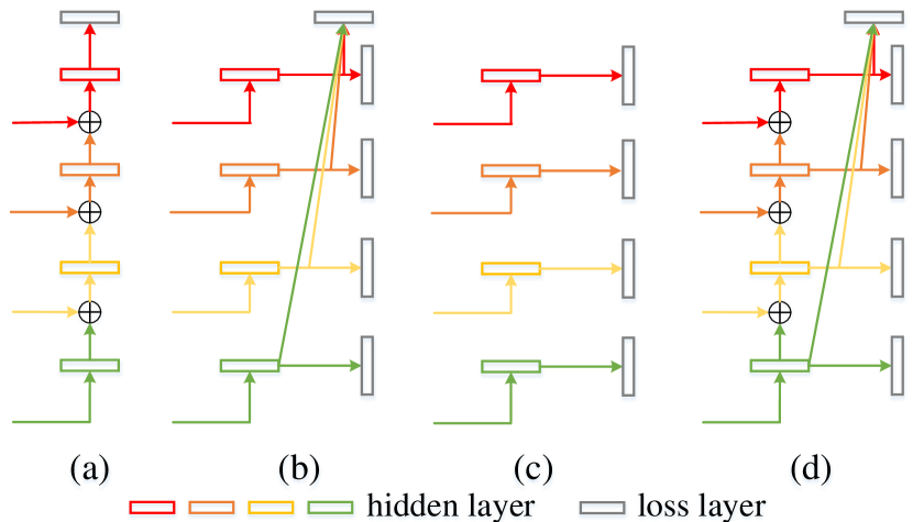
Figure 4: Different decoders.

III-E Diverse Decoders

The form of the decoder is also very important when facing different tasks. To date, many decoders (Fig. 2) with various structures have been developed. Here, we describe two of them which we found to work very well for the three binary tasks to be solved in this paper, respectively. The first one corresponds to the structure in Fig. 3a, which has been adopted by many segment detection related tasks. This structure gradually fuses the features from different side paths in a top-down manner. Since the feature channels from different side paths may vary, to perform the summation operation, a convolutional layer with kernel size $3\times 3$ is used, if needed. In spite of only one loss layer, we found that one loss layer performs better than the structure in Fig. 3d which introduces the concept of side supervision [3, 5] (See Table III). We will provide more details on the behaviors of them in the experiments sections.

For edge detection and skeleton extraction, we employ the same form of decoder as in [3] (Fig. 3c). Edge detection and skeleton extraction require the ability of sharpening thick lines detected and thereby rely more on low-level features compared to segmentation. Adding side supervision to the end of each side path allows more detailed edge information to be emphasized. On the other hand, the side predictions can also be merged with the weighted-fusion layer as the final output, providing better performance.

TABLE I: Detailed connection information between transition nodes in adjacent encoders. Here, $T_{c}^{\{1,2,3\}}$ means that current transition node gets inputs from $T_{c-1}^{1},T_{c-1}^{2},T_{c-1}^{3}$. For edge detection and skeleton extraction, all the settings are the same apart from the channels numbers in each side path. For detailed parameter information, please refer to Sec. III-F.

	Saliency			Edge & Skeleton
bottom	$S_{0}$	$S_{1}$	$S_{2}$	$S_{0}$	$S_{1}$	$S_{2}$
conv1	$T_{0}^{1}$	$T_{1}^{\{1,2,3,4,5\}}$	$T_{2}^{\{1,2,3\}}$	$T_{0}^{1}$	$T_{1}^{\{1,2,3\}}$	$T_{2}^{\{1,2,3\}}$
conv2	$T_{0}^{2}$	$T_{1}^{\{2,3,4,5,6\}}$	$T_{2}^{\{2,3,4\}}$	$T_{0}^{2}$	$T_{1}^{\{2,3,4\}}$	$T_{2}^{\{2,3,4\}}$
conv3	$T_{0}^{3}$	$T_{1}^{\{3,4,5,6\}}$	$T_{2}^{\{3,4,5\}}$	$T_{0}^{3}$	$T_{1}^{\{3,4,5\}}$	$T_{2}^{\{3,4\}}$
conv4	$T_{0}^{4}$	$T_{1}^{\{4,5,6\}}$	$T_{2}^{\{4,5\}}$	$T_{0}^{4}$	$T_{1}^{\{4,5\}}$	-
conv5	$T_{0}^{5}$	$T_{1}^{\{5,6\}}$	-	$T_{0}^{5}$	-	-
conv6	$T_{0}^{6}$	-	-	-	-	-

TABLE II: The performance of different horizontal signal flow patterns on salient object segmentation. We use the ECSSD dataset as the test set here. Pattern 1 is our detail setting. Obviously, the decrease of horizontal signal flows degrades the performance of our approach, which reflects the importance of dense connections between each pair of adjacent encoders for salient object segmentation. Note that the results listed here are without any post-processing tools.

	Pattern 1		Pattern 2		Pattern 3		Pattern 4
bottom	$S_{1}$	$S_{2}$	$S_{1}$	$S_{2}$	$S_{1}$	$S_{2}$	$S_{1}$	$S_{2}$
conv1	$T_{1}^{\{1,2,3,4,5\}}$	$T_{2}^{\{1,2,3\}}$	$T_{1}^{\{1,2,3\}}$	$T_{2}^{\{1,2,3\}}$	$T_{1}^{\{1,2\}}$	$T_{2}^{\{1,2\}}$	$T_{1}^{\{1,2,3,4\}}$	$T_{2}^{\{1,2,3\}}$
conv2	$T_{1}^{\{2,3,4,5,6\}}$	$T_{2}^{\{2,3,4\}}$	$T_{1}^{\{2,3,4\}}$	$T_{2}^{\{2,3,4\}}$	$T_{1}^{\{2,3\}}$	$T_{2}^{\{2,3\}}$	$T_{1}^{\{2,3,4,5\}}$	$T_{2}^{\{2,3,4\}}$
conv3	$T_{1}^{\{3,4,5,6\}}$	$T_{2}^{\{3,4,5\}}$	$T_{1}^{\{3,4,5\}}$	$T_{2}^{\{3,4,5\}}$	$T_{1}^{\{3,4\}}$	$T_{2}^{\{3,4\}}$	$T_{1}^{\{3,4,5,6\}}$	$T_{2}^{\{3,4,5\}}$
conv4	$T_{1}^{\{4,5,6\}}$	$T_{2}^{\{4,5\}}$	$T_{1}^{\{4,5,6\}}$	$T_{2}^{\{4,5\}}$	$T_{1}^{\{4,5\}}$	$T_{2}^{\{4,5\}}$	$T_{1}^{\{4,5,6\}}$	$T_{2}^{\{4,5\}}$
conv5	$T_{1}^{\{5,6\}}$	-	$T_{1}^{\{5,6\}}$	-	$T_{1}^{\{5,6\}}$	-	$T_{1}^{\{5,6\}}$	-
conv6	-	-	-	-	-	-	-	-
Fmeasure	0.923		0.918		0.908		0.921

TABLE III: Ablation experiments for analyzing different numbers of encoders and decoders. We use the ECSSD dataset as the test set here. The best results are highlighted in bold. No post-processing tools are used here.

#	Methods	#Encoders	Decoder	F-measure	MAE
1	DHSNet [37]	0	-	0.907	0.059
2	MSRNet [12]	0	Fig. 3a	0.913	0.054
3	GearNet (Ours)	1	Fig. 3a	0.916	0.055
4	GearNet (Ours)	2	Fig. 3b	0.918	0.053
5	GearNet (Ours)	2	Fig. 3a	0.923	0.051

III-F Implementation Details

As most prior works chose VGGNet [66] as their pre-trained model, for fair comparison, we base our model on this architecture too.

For salient object detection, we replace 3 fully-connected layers with 3 convolutional layers (conv6), the same structure to conv5. We change the stride of pool5 to 1 and the dilatation of conv6 to 2 for large receptive fields, and add 2 convolutional layers at the beginning of each side path following [5]. From side path 1 to 6, the strides are 1, 2, 4, 8, 16, and 16, respectively, and the corresponding channel numbers of convolutional layers are set to 32, 64, 128, 256, 512, and 512, respectively. We adopt the architecture shown in Table I as our default setting and the decoder in Fig. 4a as our default decoder in our experiments. For edge detection, we change the stride of pool4 layer to 1 and set the dilation rate of convolutional layers in conv5 to 2 as in [56]. The convolutional layers in each transition node are all with 16 channels by default. The connection patterns can be found in Table I. We adopt the same decoder as in [3, 56] (Fig. 4c). For skeleton extraction, the network structure is the same as in Table I aside from the channel numbers in side paths which correspond to 32, 64, 128, and 256 from side path 1 to 4, respectively. Thus, the strides of side paths 1 to 4 are 1, 2, 4, and 8, respectively. All the convolutional layers mentioned here are with kernel size 3 and stride 1.

IV Application I: Salient Object Detection

In this section, we apply the proposed approach to salient object segmentation. Salient object segmentation is an important pixel-wise binary problem and has attracted a lot of attention recently. We first describe the importance of each component in our architecture by a series of ablation experiments and then compare our method with other state-of-the-art methods.

TABLE IV: Quantitative salient object segmentation results over 5 widely used datasets. The best and the second best results in each column are highlighted in red and green, respectively. As can be seen, our approach achieves the best results on all datasets in terms of F-measure.

	Training		MSRA-B [23]		ECSSD [67]		HKU-IS [68]		DUT [69]		SOD [70, 71]
Model	#Images	Dataset	MaxF	MAE	MaxF	MAE	MaxF	MAE	MaxF	MAE	MaxF	MAE
GC [21]	-	-	0.719	0.159	0.597	0.233	0.588	0.211	0.495	0.218	0.526	0.284
DRFI [21]	2,500	MB	0.845	0.112	0.782	0.170	0.776	0.167	0.664	0.150	0.699	0.223
LEGS [31]	3,340	MB + P	0.870	0.081	0.827	0.118	0.770	0.118	0.669	0.133	0.732	0.195
MC [32]	8,000	MK	0.894	0.054	0.837	0.100	0.798	0.102	0.703	0.088	0.727	0.179
MDF [68]	2,500	MB	0.885	0.066	0.847	0.106	0.861	0.076	0.694	0.092	0.785	0.155
DCL [4]	2,500	MB	0.916	0.047	0.901	0.068	0.904	0.049	0.757	0.080	0.832	0.126
RFCN [38]	10,000	MK	-	-	0.899	0.091	0.896	0.073	0.747	0.095	0.805	0.161
DHSNET [37]	6,000	MK	-	-	0.905	0.061	0.892	0.052	-	-	0.823	0.127
ELD [36]	9,000	MK	-	-	0.865	0.098	0.844	0.071	0.719	0.091	0.760	0.154
DISC [72]	9,000	MK	0.905	0.054	0.809	0.114	0.785	0.103	0.660	0.119	-	-
MSRNet [12]	5,000	MB + H	0.930	0.042	0.913	0.054	0.916	0.039	0.785	0.069	0.847	0.112
DSS [5]	2,500	MB	0.927	0.028	0.915	0.052	0.913	0.039	0.774	0.065	0.842	0.118
UCF [40]	10,000	MK	-	-	0.844	0.069	0.823	0.061	0.621	0.120	0.800	0.164
Amulet [39]	10,000	MK	-	-	0.868	0.059	0.843	0.050	0.647	0.098	0.801	0.146
GearNet	2,500	MB	0.926	0.039	0.915	0.060	0.910	0.044	0.776	0.069	0.844	0.124
GearNet	5,000	MB + H	0.930	0.039	0.923	0.055	0.934	0.034	0.790	0.068	0.853	0.117
$\textbf{GearNet}^{\text{CRF}}$	5,000	MB + H	0.934	0.031	0.930	0.046	0.939	0.027	0.801	0.058	0.860	0.114

IV-A Evaluation Measures and Datasets

Here, we use two universally-agreed, standard, and easy-to-understand measures [27] for evaluating the existing deep saliency models. We first report the F-measure score, which simultaneously considers recall and precision, the overlapping area between the subjective ground truth annotation and the resulting prediction maps. The second measure we use is the mean absolute error (MAE) between the estimated saliency map and ground-truth annotation.

We perform evaluations on 5 datasets, including MSRA-B [23], ECSSD [67], HKU-IS [68], SOD [70, 71], and DUT-OMRON [69]. For training, we first use the 2,500 training images from MSRA-B. We also try a larger training set incorporating another 2,500 images from HKU-IS as done in [12]. Notice that all the numbers reported here are from the results the authors have presented or the results we obtained by running their publicly available code.

IV-B Ablation Studies

The hyper-parameters are as follows: weight decay (0.0005), momentum (0.9), and mini-batch size (10). The initial learning rate is set to 5e-3 and is divided by 10 after 8,000 iterations. We run the network for 12,000 iterations and choose our best model according to the performance on the validation set [23]. Further, we also use the fully connected CRF model [73] which is the same as in [5] as a post-processing tool for maintaining spatial coherence.

The Number of Encoders. The number of encoders plays an important role in our approach. Some prior works (e.g., [12, 37]) have shown good results with the decoders directly connected to the backbone. However, when we add the first encoder, a small improvement is achieved in terms of F-measure score. Quantitative results can be found in Table III. When we add another encoder, further improvements on the F-measure and MAE scores are obtained. We also added additional encoders but introducing more encoders yield no further improvements. This might be due to the fact that feature representations after two times fusion have already reached the top level of our architecture.

More Training Data. The amount of training data is essential for CNN-based methods. Besides training on the MSRA-B dataset as done in [5, 24, 4], we also attempt to add more training data as in [12]. In Table IV, we show the results using different training sets. With another 2,500 training images from [68], our performance can be further improved about 1% in terms of F-measure on average. Therefore, we believe more high-quality training data can help.

The Effect of Horizontal Signal Flows. By default, for salient object detection, we use a dense way to connect each pair of transition nodes from adjacent encoders. To show the effect of horizontal signal flows, we attempt to simplify our network by reducing the inputs of each transition node (i.e., the dash arrows in Fig. 3a). In Table II, we list four different patterns of our proposed architecture. As can be seen, when we gradually reduce the number of horizontal signal flows, the performance decreases accordingly. This phenomenon indicates that more top-down connections between transition nodes helps segmentation type tasks.

The Roles of Different Decoders. The structure of the decoder also affects the performance of our approach. We try two different structures (Figs. 3b and 3d) as our decoders. Although the structure in Fig. 3b was helpful in [5], we obtain no performance gain by such a structure but a slight decrease in F-measure (See Table III). This phenomenon reveals that introducing side supervision as in [5] is not always a good strategy for salient object segmentation. Different network architectures may favor different types of decoders.

IV-C Comparison with the State-of-the-Art

We exhaustively compare our proposed approach with 14 existing state-of-the-art salient object detection methods including 2 classic methods (GC [21] and DRFI [24]) and 10 recent CNN-based methods (LEGS [31], MC [32], MDF [68], DCL [4], RFCN [38], DHS [37], ELD [36], DISC [72], MSRNet [12], DSS [5], UCF [40], Amulet [39]). Notice that MSRNet [12] and DSS [5] are two of the best models to date. Here, our best results are shown at the bottom of Table IV.

(a) Image	(b) GT	(c) Ours	(d) DSS	(e) LEGS	(f) ELD	(g) RFCN	(h) DCL	(i) DHS

Figure 5: Visual comparisons of different salient object detection approaches.

F-measure and MAE Scores. Here, we compare our approach with the aforementioned approaches in terms of F-measure and MAE (See Table IV). As can be seen, our model trained on the MSRA-B dataset already outperforms all of the existing methods in terms of F-measure. With more training data, the results are improved further by a large margin (1% on average). This phenomenon is more pronounced when testing on the HKU-IS dataset. Notice that our approach does better than the best existing model [5, 12] using F-measure (2% improvement on average). Similar patterns can also be observed using the MAE score.

Visual Comparisons. In Fig. 5, we show the visual comparisons with several previous state-of-the-art approaches. In the top row, the source image have salient objects with complex textures. As can be seen, our approach is able to successfully segment all salient objects in images with boundaries being accurately highlighted. Some other methods such as DSS [5] and DCL [4] also produce high quality segmentation maps, although inferior to our results. A similar phenomenon also happens when processing images where contrast between foreground and background is low or when salient objects are tiny and irregular. Compared with existing methods, our approach performs much better in both cases. See for example the case shown at the bottom row of Fig. 5. These results demonstrate that our proposed horizontal hierarchy is capable of capturing rich and robust feature representations when applied to salient object detection.

V Application II: Edge Detection

In this section, we apply our GearNet to edge detection, one of the popular and basic low-level tasks in computer vision.

TABLE V: Quantitative comparison of our approach with existing edge detection methods. Here, ‘MS’ means multi-scale test as in [56]. Here, we use three scales {0.5, 1.0, 1.5, 2.0}. ‘I’ and ‘II’ correspond to the networks that are with 1 encoder and 2 encoders, respectively. The best results are highlighted in bold.

	Edge
Method	ODS	OIS
gPb-owt-ucm [46]	0.726	0.757
SE-Var [50]	0.746	0.767
MCG [74]	0.747	0.779
DeepEdge [53]	0.753	0.772
DeepContour [52]	0.756	0.773
HED [3]	0.788	0.808
CEDN [75]	0.788	0.804
RDS [76]	0.792	0.810
COB [16]	0.793	0.820
CED [77]	0.803	0.820
DCNN+sPb [55]	0.813	0.831
RCF-MS [56]	0.811	0.830
$\text{GearNet-MS}^{\mathrm{I}}$ (Ours)	0.815	0.834
$\text{GearNet-MS}^{\mathrm{II}}$ (Ours)	0.818	0.836

The hyper-parameters used in our experiment include mini-batch size set to 10, momentum set to 0.9, weight decay set to 2e-4, and initial learning rate set to 1e-6 which is divided by 10 after 23,000 iterations. Our network is trained for 30,000 iterations. We evaluate our GearNet on the Berkeley Segmentation Dataset and Benchmark (BSDS 500) [46], which is one of notable benchmarks in the edge detection field. This dataset contains 200 training, 100 validation, and 200 testing images, each with accurately annotated boundaries. Besides, our training set also incorporates the images from the PASCAL Context Dataset [78] and performs data augmentation as in [56, 3] for fair comparisons. Similar to previous works, we use the fixed contour threshold (ODS) and per-image best threshold (OIS) as our measures. Before evaluation, we apply the standard non-maximal suppression algorithm to get thinned edges.

V-A Ablation Analysis

The Number of Encoders. The number of encoders also plays an important role in the edge detection task. We consider the RCF network [56] as a special case of GearNet with 0 encoders. From Table V, we observe that adding 1 encoder (the bottom row) based on the RCF architecture helps us obtain an increase of 0.4% in terms of ODS. When we add 2 middle encoders, the ODS score can be further improved by 0.3 points. We observed no significant improvement when adding more than two encoders.

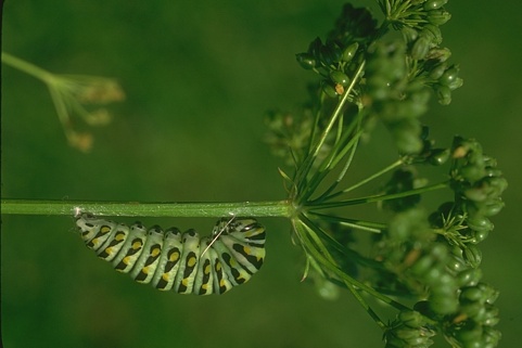
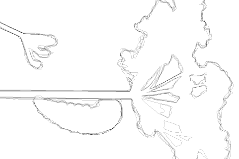
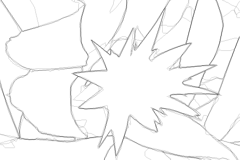
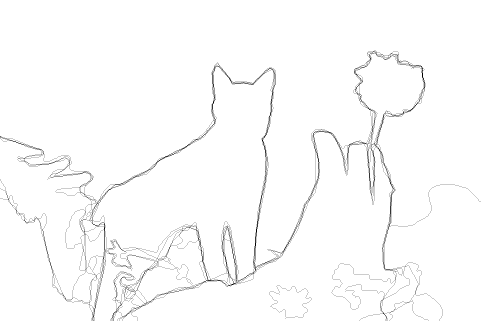
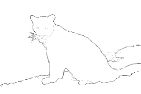
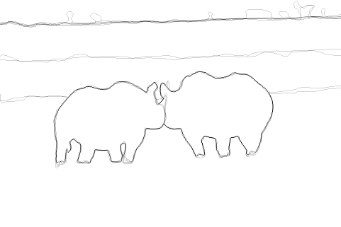
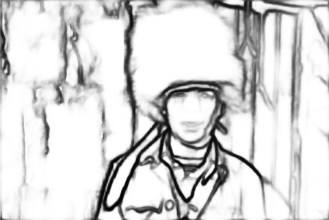
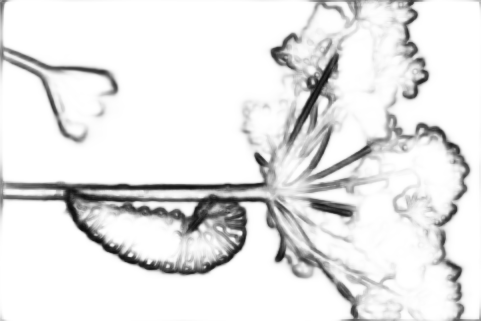
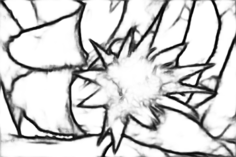
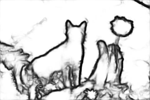
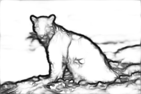
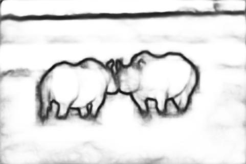
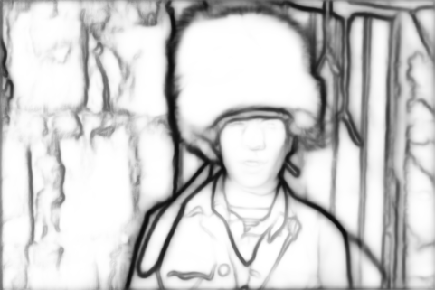
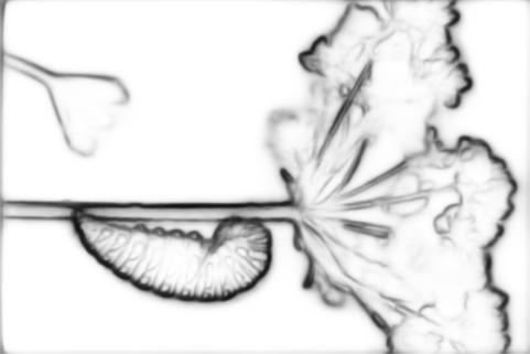
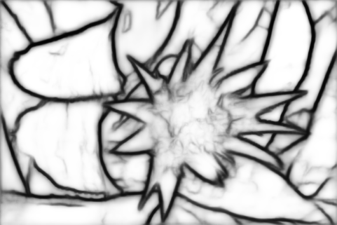
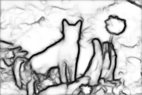
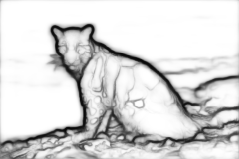
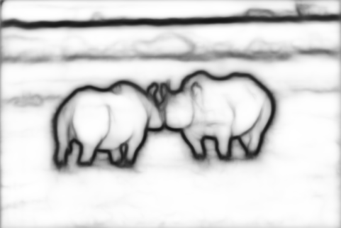
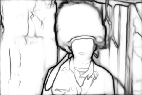
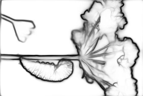
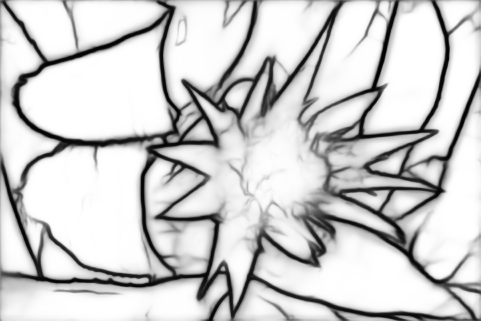
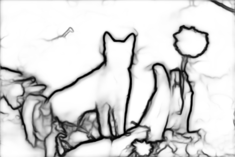
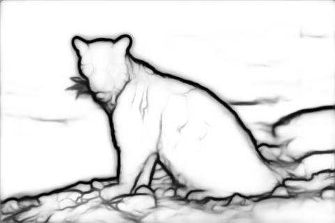
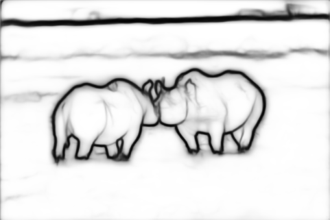
Figure 6: Visual comparisons with several recent state-of-the-art edge detectors. From top to bottom: the source images; human-annotated ground truths; results by HED [3]; results by RCF [56]; our results. As can be seen, our proposed approach is able to not only generate cleaner background but also capture weak object boundaries compared to the other two methods. This phenomenon is specially clear for the second image. All the images are from the BSDS 500 dataset [46].

The Number of Channels. As stated in Sec. III-F, the convolutional layers in each side path are all with 16 channels. To explore how the channel numbers used in each side path effect the performance of our architecture, we also attempt to increase the channel numbers as done in [56] (21 channels). However, the results show that more channels in each side path gives worse performance, leading to a decrease of around 0.2 points in terms of ODS. Similar phenomenon was also encountered when decreasing the number of channels.

TABLE VI: The results when different horizontal signal flow patterns are used for edge detection. We report both ODS score and OIS score. As can be observed, edge detection is more sensitive to the number of horizontal signal flows.

	Pattern 1		Pattern 2		Pattern 3
bottom	$S_{1}$	$S_{2}$	$S_{1}$	$S_{2}$	$S_{1}$	$S_{2}$
conv1	$T_{1}^{\{1,2,3\}}$	$T_{2}^{\{1,2\}}$	$T_{1}^{\{1,2,3\}}$	$T_{2}^{\{1\}}$	$T_{1}^{\{1,2,3,4\}}$	$T_{2}^{\{1,2,3,4\}}$
conv2	$T_{1}^{\{2,3,4\}}$	$T_{2}^{\{2,3\}}$	$T_{1}^{\{2,3,4\}}$	$T_{2}^{\{2\}}$	$T_{1}^{\{2,3,4,5\}}$	$T_{2}^{\{2,3,4\}}$
conv3	$T_{1}^{\{3,4,5\}}$	$T_{2}^{\{3,4\}}$	$T_{1}^{\{3,4,5\}}$	$T_{2}^{\{3\}}$	$T_{1}^{\{3,4,5\}}$	$T_{2}^{\{3,4\}}$
conv4	$T_{1}^{\{4,5\}}$	-	$T_{1}^{\{4,5\}}$	$T_{2}^{\{4\}}$	$T_{1}^{\{4,5\}}$	-
conv5	-	-	-	-	-	-
ODS	0.814		0.812		0.815
OIS	0.835		0.832		0.834

The Effect of Horizontal Signal Flows. We also analyze the number of horizontal signal flows in this paragraph. While more horizontal signal flows helps salient object segmentation, we found that this operation does not boost the performance in edge detection. In Table VI, we attempt to simplify our network by reducing the inputs of each transition node (Patterns 1 and 2). According to the experimental results, these two patterns degrade the performance by nearly 0.4 and 0.6 points in ODS, respectively. Furthermore, when we try to increase the number of horizontal signal flows in our architecture as in Pattern 3 in Table VI, the performance decreases as well. This demonstrates different kinds of low-level features are essential to edge detection. However, too many high-level features also harm the quality of the predicted edges because of the lack of rich detailed information.

V-B Comparison with the State-of-the-Art

We compare our results with results from 12 existing methods, including gPb-owt-ucm [46], SE-Var [50], MCG [74], DeepEdge [53], DeepContour [52], HED [3], CEDN [75], RDS [76], COB [16], CED [77], DCNN+sPb [55], and RCF-MS [56], most of which are CNN-based methods.

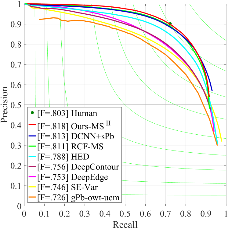
Figure 7: The precision-recall curves on BSDS 500 dataset [46].

Quantitative Analysis. In Table V, we show the quantitative results of 12 previous works as well as ours. With only one encoder, our method achieves ODS of 0.815 and OIS of 0.834, which are already better than the most of the previous works. This indicates that fusing features from different blocks of VGGNet performs better than combining only the feature maps from the same block [76]. On the other hand, more side supervision does help learning rich feature representations [16]. Furthermore, when we add another encoder to our architecture as in Table I, our results can be further enhanced from ODS of 0.815 to ODS of 0.818 $(+0.003)$. For OIS, a similar phenomenon can also be found in Table V.

Visual Analysis. In Fig. 6, we show some visual comparisons between our approach and a leading representative method [76, 3]. As can be observed, our approach performs better in detecting the boundaries compared to the other one. In Fig. 6b, it is apparent that the real boundaries of the plants are highlighted well. In addition, thanks to the fusion mechanism in our approach, the features learned by our network are much more powerful compared to [3, 76]. This is because the areas with no edges are rendered much cleaner, especially in Figs. 6a and 6b. To sum up, in spite of less than 1 point improvement compared to [76], the quality of our results is much higher visually.

PR Curve Comparisons. The precision-recall curves of some selected methods can be found in Fig. 7. One can observe that the PR-Curve produced by our approach is already better than humans in some certain cases and is better than all previous methods.

TABLE VII: Quantitative comparisons with existing skeleton extraction methods. The best results are highlighted in bold.

	Skeleton Datasets (F-measure)
Method	SK-LARGE	WH-SYMMAX
HED [3]	49.7%	73.2%
FSDS [8]	63.3%	76.9%
LMSDS [11]	64.9%	77.9%
SRN [9]	61.5%	78.0%
GearNet (Ours)	68.3%	80.1%

VI Application III: Skeleton Extraction

In this section, we apply our GearNet to skeleton extraction. We will show that our method substantially outperforms priors works by a large margin.

VI-A Ablation Analysis

The hyper-parameters we use are as follows: weight decay set to 0.0002, momentum set to 0.9, mini-batch size set to 10, and initial learning rate of 1e-6 which is divided by 10 after 20,000 iterations. We run the network for 30,000 iterations. A standard non-maximal suppression algorithm is used to obtain thinned skeletons before evaluation. We use the same training set to [11].

The Number of Encoders. As in salient object detection and edge detection, reducing the number of encoders when carrying out skeleton detection degrades the performance. When we remove the second middle encoder $\mathcal{E}_{2}$, the F-measure score drops by more than 2 points. Adding more encoders in our approach also leads to no performance gain.

The Number of Channels. In our experiment, similarly to edge detection, we also try to reduce the number of channels in each side path to half of each and observe that the results slightly decrease by 0.5 points. When we further reduce the channel numbers to a quarter of each, the performance drops dramatically (by more than 5 points). This phenomenon indicates that skeleton extraction relies on more information from the backbone. This can be achieved by adding proper number of channels in each side path. In addition, we also attempt to increase the number of channels by doubling them but find no performance gain.

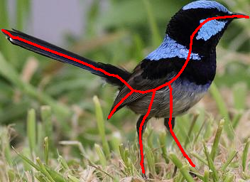
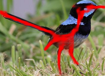
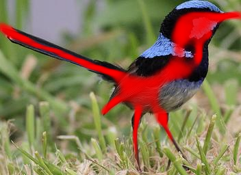
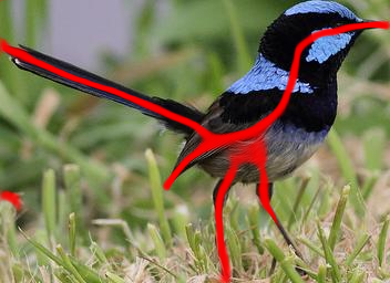
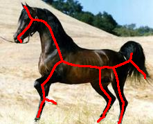
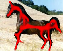
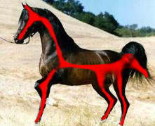
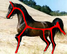
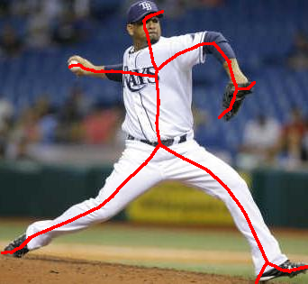
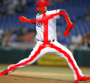
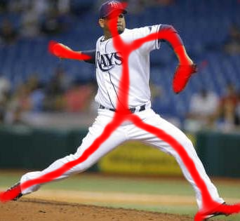
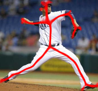
(a) GT	(b) FSDS [8]	(c) SRN [9]	(d) Ours

Figure 8: Visual comparisons with two recently representative skeleton extraction approaches. It can be easily found that our results are much thinner than the other two methods. Also, the skeletons produced by our results are continuous, which is essential for its applications.

The Effect of Horizontal Signal Flows. The number of horizontal signal flows also affects the skeleton results. We reduce the number of optional connections between $\mathcal{E}_{1}$ and $\mathcal{E}_{2}$ from 3 to 2 but the F-measure score decreases by around 2 points. Reducing the number of optional connections between $\mathcal{E}_{0}$ and $\mathcal{E}_{1}$ leads to a similar phenomenon. This indicates introducing connections between higher and lower layers is essential for skeleton detection.

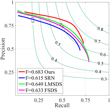
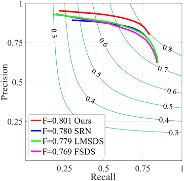
Figure 9: The precision-recall curves on SK-LARGE dataset [11] and WH-SYMMAX dataset [79]. It can be easily observed that our approach greatly outperforms existing state-of-the-art methods.

VI-B Comparison with the State-of-the-Arts

We compare our GearNet with 4 recent CNN-based methods (HED [3], FSDS [8], LMSDS [11], and SRN [9]) on 2 popular and challenging datasets including SK-LARGE [11] and WH-SYMMAX [79]. Similar to [8], we use the F-measure score to evaluate the quality of prediction maps. In Table VII, we show quantitative comparisons with existing methods. As can be seen, our method wins dramatically by a large margin (3.4 points) on the SK-LARGE dataset [8]. There is also an improvement of 2.1 points on the WH-SYMMAX dataset [79]. In Fig. 8, we also show some visual illustrations of three approaches (more can be found in our supplementary materials). Owing to the advanced features extracted from our GearNet, our method is able to more accurately locate the exact positions of the skeletons. This point can also be substantiated by the fact that our prediction maps are also much thinner than other works. Both quantitative and visual results unveil that our horizontal hierarchy provides a better way to combine different-level features for skeleton extraction.

PR Curve Comparisons In Fig. 9, we also show the precision-recall curses on two datasets, including SK-LARGE [11] and WH-SYMMAX [79]. As can be seen, quantitatively, our approach on both datasets substantially outperforms other existing methods, which verify the statement we explain above.

VII Discussion and Conclusion

In this paper, we present a novel architecture for binary vision tasks and apply it to three drastically different example tasks including salient object segmentation, edge detection, and skeleton extraction. Notice, however, that our approach is not limited to these tasks and can be potentially applied to a wide variety of binary pixel labeling tasks in computer vision. In order to take more advantage of CNNs, we introduce the concept of transition node, which receives signals from different-level features maps. Exhaustive evaluations and comparisons with recent notable state of the art methods on widely used datasets shows that our framework outperforms all of them in all three tasks, testifying the power of our proposed framework. Further, we structurally analyze our proposed architecture using several ablation experiments in each task and investigate the roles of different design choices in our approach. We hope that our work will encourage subsequent research to design universal architectures for computer vision tasks.

Qibin Hou is currently a Ph.D. Candidate with College of Computer Science and Control Engineering, Nankai University, under the supervision of Prof. Ming-Ming Cheng. His research interests include deep learning, image processing, and computer vision.

Ming-Ming Cheng received his PhD degree from Tsinghua University in 2012. Then he did 2 years research fellow, with Prof. Philip Torr in Oxford. He is now a professor at Nankai University, leading the Media Computing Lab. His research interests includes computer graphics, computer vision, and image processing. He received research awards including ACM China Rising Star Award, IBM Global SUR Award, CCF-Intel Young Faculty Researcher Program, etc.

Jiangjiang Liu is currently a Master student with College of Computer Science and Control Engineering, Nankai University, under the supervision of Prof. Ming-Ming Cheng. His research interests include deep learning, image processing, and computer vision.

Ali Borji received the PhD degree in cognitive neurosciences from the Institute for Studies in Fundamental Sciences (IPM), 2009. He is currently an assistant professor at Center for Research in Computer Vision, University of Central Florida. His research interests include visual attention, visual search, machine learning, neurosciences, and biologically plausible vision models.

Philip H.S. Torr received the PhD degree from Oxford University. After working for another 3 years at Oxford, he worked for 6 years as a research scientist for Microsoft Research, first in Redmond, then in Cambridge, founding the vision side of the Machine Learning and Perception Group. He is now a professor at Oxford University. He has won awards from several top vision conferences, including ICCV, CVPR, ECCV, NIPS, etc. He is a Royal Society Wolfson Research Merit Award holder.

References

- [1] J. Long, E. Shelhamer, and T. Darrell, “Fully convolutional networks for semantic segmentation,” in IEEE Conference on Computer Vision and Pattern Recognition, 2015, pp. 3431–3440.
- [2] H. Zhao, J. Shi, X. Qi, X. Wang, and J. Jia, “Pyramid scene parsing network,” in IEEE Conference on Computer Vision and Pattern Recognition, 2017.
- [3] S. Xie and Z. Tu, “Holistically-nested edge detection,” in IEEE International Conference on Computer Vision, 2015, pp. 1395–1403.
- [4] G. Li and Y. Yu, “Deep contrast learning for salient object detection,” in IEEE Conference on Computer Vision and Pattern Recognition, 2016.
- [5] Q. Hou, M.-M. Cheng, X. Hu, A. Borji, Z. Tu, and P. Torr, “Deeply supervised salient object detection with short connections,” in IEEE Conference on Computer Vision and Pattern Recognition, 2017.
- [6] M. Xu, Y. Liu, R. Hu, and F. He, “Find who to look at: Turning from action to saliency,” IEEE Transactions on Image Processing, vol. 27, no. 9, pp. 4529–4544, 2018.
- [7] L. Qu, S. He, J. Zhang, J. Tian, Y. Tang, and Q. Yang, “Rgbd salient object detection via deep fusion,” IEEE Transactions on Image Processing, vol. 26, no. 5, pp. 2274–2285, 2017.
- [8] W. Shen, K. Zhao, Y. Jiang, Y. Wang, Z. Zhang, and X. Bai, “Object skeleton extraction in natural images by fusing scale-associated deep side outputs,” in IEEE Conference on Computer Vision and Pattern Recognition, 2016, pp. 222–230.
- [9] W. Ke, J. Chen, J. Jiao, G. Zhao, and Q. Ye, “Srn: Side-output residual network for object symmetry detection in the wild,” arXiv preprint arXiv:1703.02243, 2017.
- [10] I. Kokkinos, “Ubernet: Training a universal convolutional neural network for low-, mid-, and high-level vision using diverse datasets and limited memory,” in IEEE Conference on Computer Vision and Pattern Recognition, 2017.
- [11] W. Shen, K. Zhao, Y. Jiang, Y. Wang, X. Bai, and A. Yuille, “Deepskeleton: Learning multi-task scale-associated deep side outputs for object skeleton extraction in natural images,” IEEE Transactions on Image Processing, vol. 26, no. 11, pp. 5298–5311, 2017.
- [12] G. Li, Y. Xie, L. Lin, and Y. Yu, “Instance-level salient object segmentation,” in IEEE Conference on Computer Vision and Pattern Recognition, 2017.
- [13] W. Wang, J. Shen, and L. Shao, “Video salient object detection via fully convolutional networks,” IEEE Transactions on Image Processing, vol. 27, no. 1, pp. 38–49, 2018.
- [14] J. Li, C. Xia, and X. Chen, “A benchmark dataset and saliency-guided stacked autoencoders for video-based salient object detection,” IEEE Transactions on Image Processing, vol. 27, no. 1, pp. 349–364, 2018.
- [15] H. Song, Z. Liu, H. Du, G. Sun, O. Le Meur, and T. Ren, “Depth-aware salient object detection and segmentation via multiscale discriminative saliency fusion and bootstrap learning,” IEEE Trans. Image Process, vol. 26, no. 9, pp. 4204–4216, 2017.
- [16] K.-K. Maninis, J. Pont-Tuset, P. Arbelaez, and L. Van Gool, “Convolutional oriented boundaries: From image segmentation to high-level tasks,” IEEE Transactions on Pattern Analysis and Machine Intelligence, 2017.
- [17] S. F. Dodge and L. J. Karam, “Visual saliency prediction using a mixture of deep neural networks,” IEEE Transactions on Image Processing, vol. 27, no. 8, pp. 4080–4090, 2018.
- [18] L. Itti, C. Koch, and E. Niebur, “A model of saliency-based visual attention for rapid scene analysis,” IEEE Transactions on Pattern Analysis and Machine Intelligence, no. 11, pp. 1254–1259, 1998.
- [19] D. A. Klein and S. Frintrop, “Center-surround divergence of feature statistics for salient object detection,” in IEEE International Conference on Computer Vision, 2011.
- [20] Y. Xie, H. Lu, and M.-H. Yang, “Bayesian saliency via low and mid level cues,” IEEE Transactions on Image Processing, vol. 22, no. 5, pp. 1689–1698, 2013.
- [21] M. Cheng, N. J. Mitra, X. Huang, P. H. Torr, and S. Hu, “Global contrast based salient region detection,” IEEE Transactions on Pattern Analysis and Machine Intelligence, 2015.
- [22] F. Perazzi, P. Krähenbühl, Y. Pritch, and A. Hornung, “Saliency filters: Contrast based filtering for salient region detection,” in IEEE Conference on Computer Vision and Pattern Recognition, 2012, pp. 733–740.
- [23] T. Liu, Z. Yuan, J. Sun, J. Wang, N. Zheng, X. Tang, and H.-Y. Shum, “Learning to detect a salient object,” IEEE Transactions on Pattern Analysis and Machine Intelligence, vol. 33, no. 2, pp. 353–367, 2011.
- [24] H. Jiang, J. Wang, Z. Yuan, Y. Wu, N. Zheng, and S. Li, “Salient object detection: A discriminative regional feature integration approach,” in IEEE Conference on Computer Vision and Pattern Recognition, 2013, pp. 2083–2090.
- [25] X. Huang and Y.-J. Zhang, “300-fps salient object detection via minimum directional contrast,” IEEE Transactions on Image Processing, vol. 26, no. 9, pp. 4243–4254, 2017.
- [26] A. Borji, M.-M. Cheng, H. Jiang, and J. Li, “Salient object detection: A survey,” arXiv preprint arXiv:1411.5878, 2014.
- [27] ——, “Salient object detection: A benchmark,” IEEE TIP, vol. 24, no. 12, pp. 5706–5722, 2015.
- [28] D.-P. Fan, J.-J. Liu, S.-H. Gao, Q. Hou, A. Borji, and M.-M. Cheng, “Salient objects in clutter: Bringing salient object detection to the foreground,” arXiv preprint arXiv:1803.06091, 2018.
- [29] S. He, R. Lau, W. Liu, Z. Huang, and Q. Yang, “Supercnn: A superpixelwise convolutional neural network for salient object detection,” International Journal of Computer Vision, vol. 115, no. 3, pp. 330–344, 2015.
- [30] G. Li and Y. Yu, “Visual saliency detection based on multiscale deep cnn features,” IEEE Transactions on Image Processing, vol. 25, no. 11, pp. 5012–5024, 2016.
- [31] L. Wang, H. Lu, X. Ruan, and M.-H. Yang, “Deep networks for saliency detection via local estimation and global search,” in IEEE Conference on Computer Vision and Pattern Recognition, 2015, pp. 3183–3192.
- [32] R. Zhao, W. Ouyang, H. Li, and X. Wang, “Saliency detection by multi-context deep learning,” in IEEE Conference on Computer Vision and Pattern Recognition, 2015, pp. 1265–1274.
- [33] R. Girshick, J. Donahue, T. Darrell, and J. Malik, “Rich feature hierarchies for accurate object detection and semantic segmentation,” in IEEE Conference on Computer Vision and Pattern Recognition, 2014, pp. 580–587.
- [34] R. Achanta, A. Shaji, K. Smith, A. Lucchi, P. Fua, and S. Süsstrunk, “Slic superpixels compared to state-of-the-art superpixel methods,” IEEE Transactions on Pattern Analysis and Machine Intelligence, vol. 34, no. 11, pp. 2274–2282, 2012.
- [35] J.-X. Zhao, R. Bo, Q. Hou, and M.-M. Cheng, “Flic: Fast linear iterative clustering with active search,” arXiv preprint arXiv:1612.01810, 2016.
- [36] L. Gayoung, T. Yu-Wing, and K. Junmo, “Deep saliency with encoded low level distance map and high level features,” in IEEE Conference on Computer Vision and Pattern Recognition, 2016.
- [37] N. Liu and J. Han, “Dhsnet: Deep hierarchical saliency network for salient object detection,” in IEEE Conference on Computer Vision and Pattern Recognition, 2016.
- [38] L. Wang, L. Wang, H. Lu, P. Zhang, and X. Ruan, “Saliency detection with recurrent fully convolutional networks,” in European Conference on Computer Vision, 2016.
- [39] P. Zhang, D. Wang, H. Lu, H. Wang, and X. Ruan, “Amulet: Aggregating multi-level convolutional features for salient object detection,” in IEEE International Conference on Computer Vision, 2017.
- [40] P. Zhang, D. Wang, H. Lu, H. Wang, and B. Yin, “Learning uncertain convolutional features for accurate saliency detection,” in IEEE International Conference on Computer Vision, 2017.
- [41] J. Canny, “A computational approach to edge detection,” IEEE Transactions on pattern analysis and machine intelligence, no. 6, pp. 679–698, 1986.
- [42] D. Marr and E. Hildreth, “Theory of edge detection,” Proceedings of the Royal Society of London B: Biological Sciences, vol. 207, no. 1167, pp. 187–217, 1980.
- [43] V. Torre and T. A. Poggio, “On edge detection,” IEEE Transactions on Pattern Analysis and Machine Intelligence, no. 2, pp. 147–163, 1986.
- [44] S. Konishi, A. L. Yuille, J. M. Coughlan, and S. C. Zhu, “Statistical edge detection: Learning and evaluating edge cues,” IEEE Transactions on Pattern Analysis and Machine Intelligence, vol. 25, no. 1, pp. 57–74, 2003.
- [45] D. R. Martin, C. C. Fowlkes, and J. Malik, “Learning to detect natural image boundaries using local brightness, color, and texture cues,” IEEE Transactions on Pattern Analysis and Machine Intelligence, vol. 26, no. 5, pp. 530–549, 2004.
- [46] P. Arbelaez, M. Maire, C. Fowlkes, and J. Malik, “Contour detection and hierarchical image segmentation,” IEEE Transactions on Pattern Analysis and Machine Intelligence, vol. 33, no. 5, pp. 898–916, 2011.
- [47] P. Dollar, Z. Tu, and S. Belongie, “Supervised learning of edges and object boundaries,” in IEEE Conference on Computer Vision and Pattern Recognition, vol. 2. IEEE, 2006, pp. 1964–1971.
- [48] X. Ren, “Multi-scale improves boundary detection in natural images,” European Conference on Computer Vision, pp. 533–545, 2008.
- [49] J. J. Lim, C. L. Zitnick, and P. Dollár, “Sketch tokens: A learned mid-level representation for contour and object detection,” in IEEE Conference on Computer Vision and Pattern Recognition, 2013, pp. 3158–3165.
- [50] P. Dollár and C. L. Zitnick, “Fast edge detection using structured forests,” IEEE Transactions on Pattern Analysis and Machine Intelligence, vol. 37, no. 8, pp. 1558–1570, 2015.
- [51] Y. Ganin and V. Lempitsky, “N^ 4-fields: Neural network nearest neighbor fields for image transforms,” in ACCV. Springer, 2014, pp. 536–551.
- [52] W. Shen, X. Wang, Y. Wang, X. Bai, and Z. Zhang, “Deepcontour: A deep convolutional feature learned by positive-sharing loss for contour detection,” in IEEE Conference on Computer Vision and Pattern Recognition, 2015, pp. 3982–3991.
- [53] G. Bertasius, J. Shi, and L. Torresani, “Deepedge: A multi-scale bifurcated deep network for top-down contour detection,” in IEEE Conference on Computer Vision and Pattern Recognition, 2015, pp. 4380–4389.
- [54] J.-J. Hwang and T.-L. Liu, “Pixel-wise deep learning for contour detection,” in ICLR, 2015.
- [55] I. Kokkinos, “Pushing the boundaries of boundary detection using deep learning,” arXiv preprint arXiv:1511.07386, 2015.
- [56] Y. Liu, M.-M. Cheng, X. Hu, K. Wang, and X. Bai, “Richer convolutional features for edge detection,” in IEEE Conference on Computer Vision and Pattern Recognition, 2017.
- [57] Z. Yu and C. Bajaj, “A segmentation-free approach for skeletonization of gray-scale images via anisotropic vector diffusion,” in IEEE Conference on Computer Vision and Pattern Recognition. IEEE, 2004.
- [58] J.-H. Jang and K.-S. Hong, “A pseudo-distance map for the segmentation-free skeletonization of gray-scale images,” in IEEE International Conference on Computer Vision. IEEE, 2001.
- [59] P. Majer, “On the influence of scale selection on feature detection for the case of linelike structures,” International Journal of Computer Vision, vol. 60, no. 3, pp. 191–202, 2004.
- [60] S. Tsogkas and I. Kokkinos, “Learning-based symmetry detection in natural images,” in European Conference on Computer Vision. Springer, 2012, pp. 41–54.
- [61] A. Sironi, V. Lepetit, and P. Fua, “Multiscale centerline detection by learning a scale-space distance transform,” in IEEE Conference on Computer Vision and Pattern Recognition, 2014.
- [62] A. Levinshtein, C. Sminchisescu, and S. Dickinson, “Multiscale symmetric part detection and grouping,” International Journal of Computer Vision, vol. 104, no. 2, pp. 117–134, 2013.
- [63] N. Widynski, A. Moevus, and M. Mignotte, “Local symmetry detection in natural images using a particle filtering approach,” IEEE Transactions on Image Processing, vol. 23, no. 12, pp. 5309–5322, 2014.
- [64] C. Peng, X. Zhang, G. Yu, G. Luo, and J. Sun, “Large kernel matters–improve semantic segmentation by global convolutional network,” in IEEE Conference on Computer Vision and Pattern Recognition, 2017.
- [65] G. Lin, A. Milan, C. Shen, and I. Reid, “Refinenet: Multi-path refinement networks for high-resolution semantic segmentation,” in IEEE Conference on Computer Vision and Pattern Recognition, 2017.
- [66] K. Simonyan and A. Zisserman, “Very deep convolutional networks for large-scale image recognition,” in ICLR, 2015.
- [67] Q. Yan, L. Xu, J. Shi, and J. Jia, “Hierarchical saliency detection,” in IEEE Conference on Computer Vision and Pattern Recognition, 2013, pp. 1155–1162.
- [68] G. Li and Y. Yu, “Visual saliency based on multiscale deep features,” in IEEE Conference on Computer Vision and Pattern Recognition, 2015, pp. 5455–5463.
- [69] C. Yang, L. Zhang, H. Lu, X. Ruan, and M.-H. Yang, “Saliency detection via graph-based manifold ranking,” in IEEE Conference on Computer Vision and Pattern Recognition, 2013, pp. 3166–3173.
- [70] D. Martin, C. Fowlkes, D. Tal, and J. Malik, “A database of human segmented natural images and its application to evaluating segmentation algorithms and measuring ecological statistics,” in IEEE International Conference on Computer Vision, vol. 2, 2001, pp. 416–423.
- [71] V. Movahedi and J. H. Elder, “Design and perceptual validation of performance measures for salient object segmentation,” in IEEE Conference on Computer Vision and Pattern Recognition, 2010, pp. 49–56.
- [72] T. Chen, L. Lin, L. Liu, X. Luo, and X. Li, “Disc: Deep image saliency computing via progressive representation learning,” IEEE TNNLS, vol. 27, no. 6, pp. 1135–1149, 2016.
- [73] P. Krähenbühl and V. Koltun, “Efficient inference in fully connected crfs with gaussian edge potentials,” in Advances in Neural Information Processing Systems, 2011.
- [74] J. Pont-Tuset, P. Arbelaez, J. T. Barron, F. Marques, and J. Malik, “Multiscale combinatorial grouping for image segmentation and object proposal generation,” IEEE Transactions on Pattern Analysis and Machine Intelligence, vol. 39, no. 1, pp. 128–140, 2017.
- [75] J. Yang, B. Price, S. Cohen, H. Lee, and M.-H. Yang, “Object contour detection with a fully convolutional encoder-decoder network,” in IEEE Conference on Computer Vision and Pattern Recognition, 2016, pp. 193–202.
- [76] Y. Liu and M. S. Lew, “Learning relaxed deep supervision for better edge detection,” in IEEE Conference on Computer Vision and Pattern Recognition, 2016, pp. 231–240.
- [77] Y. Wang, X. Zhao, and K. Huang, “Deep crisp boundaries,” in IEEE Conference on Computer Vision and Pattern Recognition, 2017, pp. 3892–3900.
- [78] R. Mottaghi, X. Chen, X. Liu, N.-G. Cho, S.-W. Lee, S. Fidler, R. Urtasun, and A. Yuille, “The role of context for object detection and semantic segmentation in the wild,” in IEEE Conference on Computer Vision and Pattern Recognition, 2014, pp. 891–898.
- [79] W. Shen, X. Bai, Z. Hu, and Z. Zhang, “Multiple instance subspace learning via partial random projection tree for local reflection symmetry in natural images,” Pattern Recognition, vol. 52, pp. 306–316, 2016.