Unconditional convergence of a fast two-level linearized algorithm for semilinear subdiffusion equations

Abstract

A fast two-level linearized scheme with unequal time-steps is constructed and analyzed for an initial-boundary-value problem of semilinear subdiffusion equations. The two-level fast L1 formula of the Caputo derivative is derived based on the sum-of-exponentials technique. The resulting fast algorithm is computationally efficient in long-time simulations because it significantly reduces the computational cost $O(MN^{2})$ and storage $O(MN)$ for the standard L1 formula to $O(MN\log N)$ and $O(M\log N)$, respectively, for $M$ grid points in space and $N$ levels in time. The nonuniform time mesh would be graded to handle the typical singularity of the solution near the time $t=0$, and Newton linearization is used to approximate the nonlinearity term. Our analysis relies on three tools: a new discrete fractional Grönwall inequality, a global consistency analysis and a discrete $H^{2}$ energy method. A sharp error estimate reflecting the regularity of solution is established without any restriction on the relative diameters of the temporal and spatial mesh sizes. Numerical examples are provided to demonstrate the effectiveness of our approach and the sharpness of error analysis.
Keywords:  semilinear subdiffusion equation; two-level L1 formula; discrete fractional Grönwall inequality; discrete $H^{2}$ energy method; unconditional convergence

1 Introduction

A two-level linearized method is considered to numerically solve the following semilinear subdiffusion equation on a bounded domain

$$\mathcal{D}^{\alpha}_{t}u =\Delta u+f(u)\quad\text{for $\boldsymbol{x}\in\Omega$ and $0<t\leqslant T$},$$ (1.1a)

$$u =u^{0}(\boldsymbol{x})\quad\text{for $\boldsymbol{x}\in\Omega$ and $t=0$},$$ (1.1b)

$$u =0\quad\text{for $\boldsymbol{x}\in\partial\Omega$ and $0<t\leqslant T$},$$ (1.1c)

where $\partial\Omega$ is the boundary of $\Omega:=(x_{l},x_{r})\times(y_{l},y_{r})$, and the nonlinear function $f(u)$ is smooth. In (1.1a) $\mathcal{D}^{\alpha}_{t}={}_{~{}0}^{C}\!\mathcal{D}_{t}^{\alpha}$ denotes the Caputo fractional derivative of order $\alpha$:

$$(\mathcal{D}^{\alpha}_{t}v)(t):=\int_{0}^{t}\omega_{1-\alpha}(t-s)v^{\prime}(s)\,\mathrm{d}{s},\quad 0<\alpha<1,$$ (1.2)

where the weakly singular kernel $\omega_{1-\alpha}(t-s)$ is defined by $\omega_{\mu}(t):=t^{\mu-1}/{\Gamma(\mu)}$. It is easy to verify $\omega_{\mu}^{\prime}(t)=\omega_{\mu-1}(t)$ and $\int_{0}^{t}\omega_{\mu}(s)\,\mathrm{d}s=\omega_{\mu+1}(t)$ for $t>0$.

In any numerical methods for solving nonlinear fractional diffusion equations (1.1a), a key consideration is the singularity of the solution near the time $t=0$, see [5, 10, 22, 17]. For example, under the assumption that the nonlinear function $f$ is Lipschitz continuous and the initial data $u^{0}\in H^{2}(\Omega)\cap H_{0}^{1}(\Omega)$, Jin et al. [5, Theorem 3.1] prove that problem (1.1) has a unique solution $u$ for which $u\in C\left([0,T];H^{2}(\Omega)\cap H_{0}^{1}(\Omega)\right)$, $\mathcal{D}^{\alpha}_{t}u\in C\left([0,T];L^{2}(\Omega)\right)$ and $\partial_{t}u\in L^{2}(\Omega)$ with $\|\partial_{t}u(t)\|_{L^{2}(\Omega)}\leq C_{u}t^{\alpha-1}$ for $0<t\leqslant T$, where $C_{u}>0$ is a constant independent of $t$ but may depend on $T$. Their analysis of numerical methods for solving (1.1) is applicable to both the L1 scheme and backward Euler convolution quadrature on a uniform time grid of diameter $\tau$; a lagging linearized technique is used to handle the nonlinearity $f(u)$, and [5, Theorem 4.5] shows that the discrete solution is $O(\tau^{\alpha})$ convergent in $L^{\infty}(L^{2}(\Omega))$.

This work may be considered as a continuation of [15], in which a sharp error estimate for the L1 formula on nonuniform meshes was obtained for linear subdiffusion-reaction equations based on a discrete fractional Grönwall inequality and a global consistency analysis. In this paper, we combine the L1 formula and the sum-of-exponentials (SOEs) technique to develop a one-step fast difference algorithm for the nonlinear subdiffusion problem (1.1) by using the Newton’s linearization to approximate nonlinear term, and present the corresponding sharp error estimate of the proposed scheme without any restriction on the relative diameters of temporal and spatial mesh sizes.

It is known that the Caputo fractional derivative involves a convolution kernel. The total number of operations required to evaluate the sum of L1 formula is proportional to $O(N^{2})$, and the active memory to $O(N)$ with $N$ representing the total time steps, which is prohibitively expensive for the practically large-scale and long-time simulations. Recently, a simple fast algorithm based on SOEs approximation is proposed to significantly reduce the computational complexity to $O(N\log N)$ and $O(\log N)$ when the final time $T\gg 1$, see [11, 4]. Another fast algorithm for the evaluation of the fractional derivative has been proposed in [1], where the compression is carried out in the Laplace domain by solving the equivalent ODE with some one-step A-stable scheme. In this paper, we develop a fast two-level L1 formula by combining a nonuniform mesh suited to the initial singularity with a fast time-stepping algorithm for the historical memory in (1.2). This scheme would be also useful to develop efficient parallel-in-time algorithms for time-fractional differential equations [20].

On the other hand, the nonlinearity of the problem also results in the difficulty for the numerical analysis. To establish an error estimate of the two-level linearized scheme at time $t_{n}$, it requires to prove the boundedness of the numerical solution at the previous time levels via $\|u^{n-1}\|_{\infty}\leqslant C_{u}$. Traditionally it is done using mathematical induction and some inverse estimate, namely,

$$\|u^{n-1}\|_{\infty}\leqslant \,\|U^{n-1}\|_{\infty}+h^{-1}\|U^{n-1}-u^{n-1}\|\leqslant\|U^{n-1}\|_{\infty}+C_{u}h^{-1}\big{(}\tau^{\beta}+h^{2}\big{)}.$$

This leads to that a time-space grid restriction $\tau=O(h^{1/\beta})$ is required in the theoretical analysis even though it is nonphysical and may be unnecessary in numerical simulations. In this paper, we will extend the discrete $H^{2}$ method developed in [14, 12, 13] to prove unconditional convergence of our fully discrete solution without the restriction conditions of between mesh sizes $\tau$ and $h$ comparing with the traditional method. The main idea of discrete $H^{2}$ energy method is to separately treat the temporal and spatial truncation errors. This simple implementation avoids some nonphysical time-space grid restrictions in the error analysis. A related approach in a finite element setting are discussed in [7, 8, 9].

The convergence rate of L1 formula for the Caputo derivative is limited by the smoothness of the solution. The analysis here is based on the following assumptions on the solution

$$\left\|u\right\|_{H^{4}(\Omega)}\leqslant C_{u},\;\left\|\partial_{t}u\right\|_{H^{4}(\Omega)}\leqslant C_{u}(1+t^{\sigma-1})\text{ and }\left\|\partial_{tt}u\right\|_{H^{2}(\Omega)}\leqslant C_{u}(1+t^{\sigma-2})$$ (1.3)

for $0<t\leq T$, where $\sigma\in(0,1)\cup(1,2)$ is a regularity parameter. To resolve the singularity at $t=0$, it is reasonable to use a nonuniform mesh that concentrates grid points near $t=0$, see [2, 3, 15, 19]. We make the following assumption on the time mesh:

AssG.

Let $\gamma\geq 1$ be a user-chosen parameter. There is a constant $C_{\gamma}>0$, independent of $k$, such that $\tau_{k}\leq C_{\gamma}\tau\min\{1,t_{k}^{1-1/\gamma}\}$ for $1\leq k\leq N$ and $t_{k}\leqslant C_{\gamma}t_{k-1}$ for $2\leq k\leq N$.

Since $\tau_{1}=t_{1}$, AssG implies that $\tau_{1}=O(\tau^{\gamma})$, while for those $t_{k}$ bounded away from $t=0$ one has $\tau_{k}=O(\tau)$. The parameter $\gamma$ controls the extent to which the grid points are concentrated near $t=0$: increasing $\gamma$ will decrease the time-step sizes near $t=0$ and so move mesh points closer to $t=0$. A simple example of a family of meshes satisfying AssG is the graded grid $t_{k}=T(k/N)^{\gamma}$, which is discussed in [2, 15, 19]. Although nonuniform meshes are flexible and reasonably convenient for practical implementation, they can significantly complicate the numerical analysis of schemes, both with respect to stability and consistency. In this paper, our analysis will rely on a generalized fractional Grönwall inequality [16], which would be applicable for any discrete fractional derivatives having the discrete convolution form.

Throughout the paper, any subscripted $C$, such as $C_{u}$, $C_{\gamma}$, $C_{\Omega}$, $C_{v}$, $C_{0}$ and $C_{F}$, denotes a generic positive constant, not necessarily the same at different occurrences, which is always dependent on the given data and the solution but independent of the time-space grid steps. The paper is organized as follows. Section 2 presents the two-level fast L1 formula and the corresponding linearized fast scheme. The global consistency analysis of fast L1 formula and the Newton’s linearization is presented in Section 3. A sharp error estimate for the linearized fast scheme is proved in Section 4. Two numerical examples in Section 5 are given to demonstrate the sharpness of our analysis.

2 A two-level fast method

We approximate the Caputo fractional derivative (1.2) on a (possibly nonuniform) time mesh $0=t_{0}<\cdots<t_{k-1}<t_{k}<\cdots<t_{N}=T$, with the time-step sizes $\tau_{k}:=t_{k}-t_{k-1}$ for $1\leq k\leq N$, the maximum time-step $\tau=\max_{1\leqslant k\leqslant N}\tau_{k}$ and the step size ratios $\rho_{k}:=\tau_{k}/\tau_{k+1}$ for $1\leq k\leq N-1$. In space we use a standard finite difference method on a tensor product grid. Let $M_{1}$ and $M_{2}$ be two positive integers. Set $h_{1}=(x_{r}-x_{l})/M_{1},\ h_{2}=(y_{r}-y_{l})/M_{2}$ and the maximum spatial length $h=\max\{h_{1},h_{2}\}$. Then the fully discrete spatial grid $\bar{\Omega}_{h}:=\{\boldsymbol{x}_{h}=(x_{l}+ih_{1},y_{l}+jh_{2})\,|\,0\leqslant i\leqslant M_{1},0\leqslant j\leqslant M_{2}\}$. Set ${\Omega}_{h}=\bar{\Omega}_{h}\cap\Omega$ and the boundary $\partial\Omega_{h}=\bar{\Omega}_{h}\cap\partial\Omega$. Given a grid function $v=\{v_{ij}\}$, define

$$v_{i-\frac{1}{2},j}=\left(v_{i,j}+v_{i-1,j}\right)/{2},\ \delta_{x}v_{i-\frac{1}{2},j}=\left(v_{i,j}-v_{i-1,j}\right)/{h_{1}},\ \delta_{x}^{2}v_{ij}=\big{(}\delta_{x}v_{i+\frac{1}{2},j}-\delta_{x}v_{i-\frac{1}{2},j}\big{)}/{h_{1}}.$$

Difference operators $v_{i,j-\frac{1}{2}},\ \delta_{y}v_{i,j-\frac{1}{2}},\ \delta_{x}\delta_{y}v_{i-\frac{1}{2},j-\frac{1}{2}}$ and $\delta_{y}^{2}v_{ij}$ can be defined analogously. The second-order approximation of $\Delta v(\boldsymbol{x}_{h})$ for $\boldsymbol{x}_{h}\in\Omega_{h}$ is $\Delta_{h}v_{h}:=(\delta_{x}^{2}+\delta_{y}^{2})v_{h}$. Let $\mathcal{V}_{h}$ be the space of grid functions, $\mathcal{V}_{h}=\big{\{}v=\left(v_{h}\right)_{\boldsymbol{x}_{h}\in\bar{\Omega}_{h}}\,\big{|}\,v_{h}=0\;\mbox{for}\;\boldsymbol{x}_{h}\in\partial\Omega_{h}\big{\}}$. For $v,w\in\mathcal{V}_{h}$, define the discrete inner product $\left\langle v,w\right\rangle=h_{1}h_{2}\sum_{\boldsymbol{x}_{h}\in\Omega_{h}}v_{h}w_{h}$, the $L^{2}$ norm $\|v\|=\sqrt{\left\langle v,v\right\rangle}$, the $H^{1}$ seminorm $\|\nabla_{h}v\|=\sqrt{\|\delta_{x}v\|^{2}+\|\delta_{y}v\|^{2}}$ and the maximum norm $\|v\|_{\infty}=\max_{\boldsymbol{x}_{h}\in\Omega_{h}}\left|v_{h}\right|$. For any $v\in\mathcal{V}_{h}$, by [14, Lemmas 2.1, 2.2 and 2.5] there exists a constant $C_{\Omega}>0$ such that

$$\|v\|\leqslant C_{\Omega}\|\nabla_{h}v\|,\quad\|\nabla_{h}v\|\leqslant C_{\Omega}\|\Delta_{h}v\|,\quad\|v\|_{\infty}\leqslant C_{\Omega}\|\Delta_{h}v\|.$$ (2.1)

2.1 A fast variant of the L1 formula

On our nonuniform mesh, the standard L1 approximation of the Caputo derivative is

$$(D^{\alpha}_{\tau}v)^{n}:=\sum_{k=1}^{n}\frac{1}{\tau_{k}}\int_{t_{k-1}}^{t_{k}}\omega_{1-\alpha}(t_{n}-s)\nabla_{\tau}v^{k}\,\mathrm{d}s=\sum_{k=1}^{n}a_{n-k}^{(n)}\nabla_{\tau}v^{k}\,,$$ (2.2)

where $\nabla_{\tau}v^{k}:=v^{k}-v^{k-1}$ and the convolution kernel $a_{n-k}^{(n)}$ is defined by

$$a_{n-k}^{(n)}:=\frac{1}{\tau_{k}}\int_{t_{k-1}}^{t_{k}}\!\!\omega_{1-\alpha}(t_{n}-s)\,\mathrm{d}s=\frac{1}{\tau_{k}}\left[\omega_{2-\alpha}(t_{n}-t_{k-1})-\omega_{2-\alpha}(t_{n}-t_{k})\right],\quad 1\leqslant k\leqslant n.$$ (2.3)

Lemma 2.1

For fixed integer $n\geq 2$, the convolution kernel $a^{(n)}_{n-k}$ of (2.3) satisfies

• $\displaystyle a_{n-k-1}^{(n)}>\omega_{1-\alpha}(t_{n}-t_{k})>a_{n-k}^{(n)},\quad 1\leqslant k\leqslant n-1;$

• $\displaystyle a^{(n)}_{n-k-1}-a^{(n)}_{n-k}>\tfrac{1}{2}\left[\omega_{1-\alpha}(t_{n}-t_{k})-\omega_{1-\alpha}(t_{n}-t_{k-1})\right],\quad 1\leqslant k\leqslant n-1.$

Proof  The integral mean-value theorem yields (i) directly; see [22, 15]. For any function $q\in C^{2}[t_{k-1},t_{k}]$, let $\Pi_{1,k}q$ be the linear interpolant of $q(t)$ at $t_{k-1}$ and $t_{k}$. Let $\widetilde{\Pi_{1,k}}q:=q-\Pi_{1,k}q$ be the error in this interpolant. For $q(s)=\omega_{1-\alpha}(t_{n}-s)$ one has $q^{\prime\prime}(s)=\omega_{-\alpha-1}(t_{n}-s)>0$ for $0<s<t_{n}$, so the Peano representation of the interpolation error [15, Lemma 3.1] shows that $\int_{t_{k-1}}^{t_{k}}\big{(}\widetilde{\Pi_{1,k}}q\big{)}(s)\,\mathrm{d}s<0$. Thus the definition (2.3) of $a^{(n)}_{n-k}$ yields

$$a^{(n)}_{n-k}-\frac{1}{2}\omega_{1-\alpha}(t_{n}-t_{k})-\frac{1}{2}\omega_{1-\alpha}(t_{n}-t_{k-1})=\frac{1}{\tau_{k}}\int_{t_{k-1}}^{t_{k}}\big{(}\widetilde{\Pi_{1,k}}q\big{)}(s)\,\mathrm{d}s<0,\quad 1\leqslant k\leqslant n-1.$$

Subtract this inequality from (i) to obtain (ii) immediately.   

As the L1 formula (2.2) involves the solution at all previous time-levels, it is computationally inefficient to directly evaluate it when solving the fractional diffusion problem (1.1) using time-stepping. We therefore use the SOEs approach of [4, 11, 21] to develop a fast L1 formula. A basic result of the SOE approximation (see [4, Theorem 2.5] or [21, Lemma 2.2]) is the following:

Lemma 2.2

Given $\alpha\in(0,1)$, an absolute tolerance error $\epsilon\ll 1$, a cut-off time $\Delta{t}>0$ and a final time $T$, there exists a positive integer $N_{q}$, positive quadrature nodes $\theta^{\ell}$ and positive weights $\varpi^{\ell}$ $(1\leqslant\ell\leqslant N_{q})$ such that

$$\Big{|}\omega_{1-\alpha}(t)-\sum_{\ell=1}^{N_{q}}\varpi^{\ell}e^{-\theta^{\ell}t}\Big{|}\leqslant\epsilon\quad\forall\,t\in[\Delta{t},T],$$

where the number $N_{q}$ of quadrature nodes satisfies

$$N_{q}=O\left(\log\frac{1}{\epsilon}\Big{(}\log\log\frac{1}{\epsilon}+\log\frac{T}{\Delta{t}}\Big{)}+\log\frac{1}{\Delta{t}}\Big{(}\log\log\frac{1}{\epsilon}+\log\frac{1}{\Delta{t}}\Big{)}\right).$$

After that, we divide the fractional Caputo derivative $(\mathcal{D}^{\alpha}_{t}v)(t_{n})$ of (1.2) into a sum of a local part (an integral over $[t_{n-1},t_{n}]$) and a history part (an integral over $[0,t_{n-1}]$), then approximate $v^{\prime}$ by linear interpolation in the local part (similar to the standard L1 method) and use the SOE technique of Lemma 2.2 to approximate the kernel $\omega_{1-\alpha}(t-s)$ in the history part. It yields

$$\big{(}\mathcal{D}^{\alpha}_{t}u\big{)}(t_{n})\approx \,\int_{t_{n-1}}^{t_{n}}\omega_{1-\alpha}(t_{n}-s)\frac{\nabla_{\tau}u^{n}}{\tau_{n}}\,\mathrm{d}s+\int_{0}^{t_{n-1}}\sum_{\ell=1}^{N_{q}}\varpi^{\ell}e^{-\theta^{\ell}(t_{n}-s)}u^{\prime}(s)\,\mathrm{d}s$$

$$= \,a_{0}^{(n)}\nabla_{\tau}u^{n}+\sum_{\ell=1}^{N_{q}}\varpi^{\ell}e^{-\theta^{\ell}\tau_{n}}\mathcal{H}^{\ell}(t_{n-1}),\quad n\geq 1,$$

where $\mathcal{H}^{\ell}(t_{k}):=\int_{0}^{t_{k}}e^{-\theta^{\ell}(t_{k}-s)}u^{\prime}(s)\,\mathrm{d}s$ with $\mathcal{H}^{\ell}(t_{0})=0$ for $1\leqslant\ell\leqslant N_{q}\,$. To compute $\mathcal{H}^{\ell}(t_{k})$ efficiently we apply linear interpolation in each cell $[t_{k-1},t_{k}]$, obtaining

$$\mathcal{H}^{\ell}(t_{k})= \,e^{-\theta^{\ell}\tau_{k}}\mathcal{H}^{\ell}(t_{k-1})+\int_{t_{k-1}}^{t_{k}}e^{-\theta^{\ell}(t_{k}-s)}u^{\prime}(s)\,\mathrm{d}s\approx e^{-\theta^{\ell}\tau_{k}}\mathcal{H}^{\ell}(t_{k-1})+b^{(k,\ell)}\nabla_{\tau}u^{k},$$

where the positive coefficient is given by

$$b^{(k,\ell)}:=\frac{1}{\tau_{k}}\int_{t_{k-1}}^{t_{k}}e^{-\theta^{\ell}(t_{k}-s)}\,\mathrm{d}s,\quad k\geq 1,\;1\leqslant\ell\leqslant N_{q}\,.$$ (2.4)

In summary, we now have the two-level fast L1 formula

$$(D^{\alpha}_{f}u)^{n}:=a_{0}^{(n)}\nabla_{\tau}u^{n}+\sum_{\ell=1}^{N_{q}}\varpi^{\ell}e^{-\theta^{\ell}\tau_{n}}H^{\ell}(t_{n-1}),\quad n\geq 1,$$ (2.5a)

where $$H^{\ell}(t_{k}) H^{\ell}(t_{0})=0$$ satisfies and the recurrence relationship

$$H^{\ell}(t_{k})=e^{-\theta^{\ell}\tau_{k}}H^{\ell}(t_{k-1})+b^{(k,\ell)}\nabla_{\tau}u^{k},\quad k\geq 1,\;1\leqslant\ell\leqslant N_{q}\,.$$ (2.5b)

2.2 The two-level linearized scheme

Write $U_{h}^{n}=u(\boldsymbol{x}_{h},t_{n})$ for $\boldsymbol{x}_{h}\in\bar{\Omega}_{h}$, $0\leqslant n\leqslant N$. Let $u_{h}^{n}$ be the discrete approximation of $U_{h}^{n}$. Using the fast L1 formula (2.5) and Newton linearization, we obtain a linearized scheme for the problem (1.1): find $\{u_{h}^{N}\}\in\mathcal{V}_{h}$ such that

$$(D^{\alpha}_{f}u_{h})^{n}= \,\Delta_{h}u_{h}^{n}+f(u_{h}^{n-1})+f^{\prime}(u_{h}^{n-1})\nabla_{\tau}u_{h}^{n}\,,\quad\boldsymbol{x}_{h}\in\Omega_{h},\;1\leqslant n\leqslant N;$$ (2.6a)

$$u_{h}^{0}= \,u^{0}(\boldsymbol{x}_{h}),\quad\boldsymbol{x}_{h}\in\bar{\Omega}_{h}\,.$$ (2.6b)

Note that, the Newton linearization of a general nonlinear function $f=f(\boldsymbol{x},t,u)$ at $t=t_{n}$ takes the form $f(\boldsymbol{x}_{h},t_{n},u_{h}^{n})\approx f(\boldsymbol{x}_{h},t_{n},u_{h}^{n-1})+f_{u}^{\prime}(\boldsymbol{x}_{h},t_{n},u_{h}^{n-1})\nabla_{\tau}u_{h}^{n}\,.$ The scheme (2.6) is a two-level procedure for computing $\{u_{h}^{n}\}$, since (2.6a) can be reformulated as

$$\left[a_{0}^{(n)}-\Delta_{h}-f^{\prime}(u_{h}^{n-1})\right]\nabla_{\tau}u_{h}^{n}= \,\Delta_{h}u_{h}^{n-1}+f(u_{h}^{n-1})-\sum_{\ell=1}^{N_{q}}\varpi^{\ell}e^{-\theta^{\ell}\tau_{n}}H_{h}^{\ell}(t_{n-1}),$$ (2.7)

$$H_{h}^{\ell}(t_{n})= \,e^{-\theta^{\ell}\tau_{n}}H_{h}^{\ell}(t_{n-1})+b^{(n,\ell)}\nabla_{\tau}u_{h}^{n}\,,\quad 1\leqslant\ell\leqslant N_{q}.$$ (2.8)

Thus, once the solution $\{u_{h}^{n-1},\;H_{h}^{\ell}(t_{n-1})\}$ at the previous time-level $t_{n-1}$ is available, the current solution $\{u_{h}^{n}\}$ can be found by (2.7) with a fast matrix solver and the historic term $\{H_{h}^{\ell}(t_{n})\}$ will be updated explicitly by the recurrence formula (2.8).

Remark 2.3

At each time level the scheme (2.6) requires $O(MN_{q})$ storage and $O(MN_{q})$ operations, where $M=M_{1}M_{2}$ is the total number of spatial grid points. Given a tolerance error $\epsilon=\epsilon_{0}$, by virtue of Lemma 2.2, the number of quadrature nodes $N_{q}=O(\log N)$ if the final time $T\gg 1$. Hence our new method is computationally efficient since it computes the final solution using in total $O(M\log N)$ storage and $O(MN\log N)$ operations.

2.3 Discrete fractional Grönwall inequality

Our analysis relies on a generalized discrete fractional Grönwall inequality [16], which is applicable for any discrete fractional derivative having the discrete convolution form

$$(\mathcal{D}^{\alpha}_{t}v)^{n}\approx\sum_{k=1}^{n}A^{(n)}_{n-k}(v^{k}-v^{k-1}),\quad 1\leqslant n\leqslant N,$$ (2.9)

provided that $A^{(n)}_{n-k}$ and the time-steps $\tau_{n}$ satisfy the following three assumptions:

Ass1.

The discrete kernel is monotone, that is, $A^{(n)}_{k-2}\geq A^{(n)}_{k-1}>0$ for $2\leqslant k\leqslant n\leqslant N$.

Ass2.

There is a constant $\pi_{A}>0$ such that $A^{(n)}_{n-k}\geq\frac{1}{\pi_{A}}\int_{t_{k-1}}^{t_{k}}\frac{\omega_{1-\alpha}(t_{n}-s)}{\tau_{k}}\,\mathrm{d}{s}$ for $1\leq k\leq n\leqslant N$.

Ass3.

There is a constant $\rho>0$ such that the time-step ratios $\rho_{k}\leq\rho$ for $1\leq k\leq N-1$.

The complementary discrete kernel $P^{(n)}_{n-k}$ was introduced by Liao et al. [15, 16]; it satisfies the following identity

$$\sum_{j=k}^{n}P^{(n)}_{n-j}A^{(j)}_{j-k}\equiv 1\quad\text{for $1\leq k\leq n\leq N$.}$$ (2.10)

Rearranging this identity yields a recursive formula that defines $P^{(n)}_{n-k}$ :

$$P_{0}^{(n)}:=1/{A_{0}^{(n)}},\quad P_{n-j}^{(n)}:=1/{A_{0}^{(j)}}\sum_{k=j+1}^{n}\Big{(}A_{k-j-1}^{(k)}-A_{k-j}^{(k)}\Big{)}P_{n-k}^{(n)}\,,\quad 1\leqslant j\leqslant n-1.$$ (2.11)

From [16, Lemma 2.2] we see that $P^{(n)}_{n-k}$ is well-defined and non-negative if the assumption Ass1 holds true. Furthermore, if Ass2 holds true, then

$$\sum_{j=1}^{n}P^{(n)}_{n-j}\leqslant\pi_{A}\,\omega_{1+\alpha}(t_{n})\quad\text{for $1\leq n\leq N$.}$$ (2.12)

Recall that the Mittag–Leffler function $E_{\alpha}(z)=\sum_{k=0}^{\infty}\frac{z^{k}}{\Gamma(1+k\alpha)}$. We state the following (slightly simplified) version of [16, Theorem 3.2]. This result differs substantially from the fractional Grönwall inequality of Jin et al. [5, Theorem 4] since it is valid on very general nonuniform time meshes.

Theorem 2.4

Let Ass1–Ass3 hold true. Suppose that the sequences $(\xi_{1}^{n})_{n=1}^{N}$, $(\xi_{2}^{n})_{n=1}^{N}$ are nonnegative. Assume that $\lambda_{0}$ and $\lambda_{1}$ are non-negative constants and the maximum step size $\tau\leqslant 1/\sqrt[\alpha]{2\max\{1,\rho\}\pi_{A}\Gamma(2-\alpha)(\lambda_{0}+\lambda_{1})}$. If the nonnegative sequence $(v^{k})_{k=0}^{N}$ satisfies

$$\sum_{k=1}^{n}A^{(n)}_{n-k}\nabla_{\tau}v^{k}\leq\lambda_{0}v^{n}+\lambda_{1}v^{n-1}+\xi_{1}^{n}+\xi_{2}^{n}\quad\text{for $1\leq n\leq N$,}$$ (2.13)

then it holds that for $1\leq n\leq N$,

$$v^{n}\leq 2E_{\alpha}\big{(}2\max\{1,\rho\}\pi_{A}(\lambda_{0}+\lambda_{1})t_{n}^{\alpha}\big{)}\biggl{(}v^{0}+\max_{1\leq k\leq n}\sum_{j=1}^{k}P^{(k)}_{k-j}\xi_{1}^{j}+\pi_{A}\omega_{1+\alpha}(t_{n})\max_{1\leq j\leq n}\xi_{2}^{j}\biggr{)}.$$ (2.14)

To facilitate our analysis, we now eliminate the historic term $H^{\ell}(t_{n})$ from the fast L1 formula (2.5a) for $(D^{\alpha}_{f}u)^{n}$. From the recurrence relationship (2.5b), it is easy to see that

$$H^{\ell}(t_{k})=\sum_{j=1}^{k}e^{-\theta^{\ell}(t_{k}-t_{j})}b^{(j,\ell)}\nabla_{\tau}u^{j},\quad k\geq 1,\;1\leqslant\ell\leqslant N_{q}.$$

Inserting this in (2.5a) and using the definition (2.4), one obtains the alternative formula

$$(D^{\alpha}_{f}u)^{n}= \,a_{0}^{(n)}\nabla_{\tau}u^{n}+\sum_{k=1}^{n-1}\frac{\nabla_{\tau}u^{k}}{\tau_{k}}\int_{t_{k-1}}^{t_{k}}\sum_{\ell=1}^{N_{q}}\varpi^{\ell}e^{-\theta^{\ell}(t_{n}-s)}\,\mathrm{d}s=\sum_{k=1}^{n}A_{n-k}^{(n)}\nabla_{\tau}u^{k},\quad n\geq 1,$$ (2.15)

where the discrete convolution kernel $A_{n-k}^{(n)}$ is henceforth defined by

$$A_{0}^{(n)}:=a_{0}^{(n)},\quad A_{n-k}^{(n)}:=\frac{1}{\tau_{k}}\int_{t_{k-1}}^{t_{k}}\sum_{\ell=1}^{N_{q}}\varpi^{\ell}e^{-\theta^{\ell}(t_{n}-s)}\,\mathrm{d}s,\quad 1\leqslant k\leqslant n-1,\;n\geq 1.$$ (2.16)

The formula (2.15) takes the form of (2.9), and we now verify that our $A_{n-k}^{(n)}$ defined by (2.16) satisfy Ass1 and Ass2, allowing us to apply Theorem 2.4 and establish the convergence of our computed solution. Part (I) of the next lemma ensures that Ass1 is valid, while part (II) implies that Ass2 holds true with $\pi_{A}=\frac{3}{2}$.

Lemma 2.5

If the tolerance error $\epsilon$ of SOE satisfies $\epsilon\leqslant\min\left\{\frac{1}{3}\omega_{1-\alpha}(T),\alpha\,\omega_{2-\alpha}(1)\right\}$, then the discrete convolutional kernel $A_{n-k}^{(n)}$ of (2.16) satisfies

• $A_{k-1}^{(n)}>A_{k}^{(n)}>0,\;\;1\leqslant k\leqslant n-1;$ (II) $A_{0}^{(n)}=a_{0}^{(n)}$ and $A_{n-k}^{(n)}\geq\frac{2}{3}a_{n-k}^{(n)},\;\;1\leqslant k\leqslant n-1.$

Proof  The definition (2.3) and Lemma 2.1 (i) yield

$$a_{0}^{(n)}-a_{1}^{(n)}>a_{0}^{(n)}-\omega_{1-\alpha}(\tau_{n})=\tfrac{\alpha}{\tau_{n}}\omega_{2-\alpha}(\tau_{n})\geq\alpha\,\omega_{2-\alpha}(1)\geq\epsilon\,,$$

where the step size $\tau_{n}\leqslant 1$ and our hypothesis on $\epsilon$ are used. The definition (2.16) and Lemma 2.2 imply that $A_{0}^{(n)}=a_{0}^{(n)}>a_{1}^{(n)}+\epsilon>A_{1}^{(n)}$. Lemma 2.2 also shows that $\theta^{\ell},\varpi^{\ell}>0$ for $\ell=1,\dots,N_{q}$; the mean-value theorem now yields property (I). By Lemma 2.1 (i) and our hypothesis on $\epsilon$ we have $\epsilon\leqslant\frac{1}{3}\omega_{1-\alpha}(t_{n}-t_{k-1})<\frac{1}{3}a_{n-k}^{(n)}$ for $1\leqslant k\leqslant n-1$. Hence Lemma 2.2 gives $A_{n-k}^{(n)}\geq a_{n-k}^{(n)}-\epsilon\geq\frac{2}{3}a_{n-k}^{(n)}$ for $1\leqslant k\leqslant n-1$. The proof is complete.   

3 Global consistency error analysis

We now proceed with the consistency error analysis of our fast linearized method, and begin with the consistency error of the standard L1 formula $(D^{\alpha}_{\tau}u)^{n}$ of (2.2).

Lemma 3.1

For $v\in C^{2}(0,T]$ with $\int_{0}^{T}t\,|v^{\prime\prime}(t)|\,\mathrm{d}s<\infty$, one has

$$\big{|}(\mathcal{D}^{\alpha}_{t}v)(t_{n})-(D^{\alpha}_{\tau}v)^{n}\big{|}\leqslant a_{0}^{(n)}G^{n}+\sum_{k=1}^{n-1}\big{(}a_{n-k-1}^{(n)}-a_{n-k}^{(n)}\big{)}G^{k},\quad n\geq 1,$$

where the L1 kernel $a_{n-k}^{(n)}$ is defined by (2.3) and $G^{k}:=2\int_{t_{k-1}}^{t_{k}}\left(t-t_{k-1}\right)\left|v^{\prime\prime}(t)\right|\,\mathrm{d}t$.

Proof  From Taylor’s formula with integral remainder, the truncation error of the standard L1 formula at time $t=t_{n}$ is (see [15, Lemma 3.3])

$$(\mathcal{D}^{\alpha}_{t}v)(t_{n})-(D^{\alpha}_{\tau}v)^{n}= \,\sum_{k=1}^{n}\int_{t_{k-1}}^{t_{k}}\omega_{1-\alpha}(t_{n}-s)\left(v^{\prime}(s)-\nabla_{\tau}v^{k}/\tau_{k}\right)\,\mathrm{d}s$$

$$= \,\sum_{k=1}^{n}\int_{t_{k-1}}^{t_{k}}v^{\prime\prime}(t)\,\big{(}\widetilde{\Pi_{1,k}}Q\big{)}(t)\,\mathrm{d}{t}\,,\quad n\geq 1,$$ (3.1)

where $Q(t)=\omega_{2-\alpha}(t_{n}-t)$ and we use the notation of the proof of Lemma 2.1. By the error formula for linear interpolation [15, Lemma 3.1], we have

$$\big{(}\widetilde{\Pi_{1,k}}Q\big{)}(t)=\int_{t_{k-1}}^{t_{k}}\chi_{k}(t,y)Q^{\prime\prime}(y)\,\mathrm{d}{y},\quad t_{k-1}<t<t_{k},\;1\leqslant k\leqslant n,$$

where the Peano kernel $\chi_{k}(t,y)=\max\{t-y,0\}-\frac{t-t_{k-1}}{\tau_{k}}(t_{k}-y)$ satisfies

$$-\tfrac{t-t_{k-1}}{\tau_{k}}(t_{k}-t)\leqslant\chi_{k}(t,y)<0\qquad\text{for any $t,y\in(t_{k-1},t_{k}).$}$$

Observing that for each fixed $n\geq 1$ the function $Q$ is decreasing and $Q^{\prime\prime}(t)=\omega_{-\alpha}(t_{n}-t)<0$, we arrive at the interpolation error $\big{(}\widetilde{\Pi_{1,k}}Q\big{)}(t)\geq 0$ for $1\leqslant k\leqslant n$, with

$$\big{(}\widetilde{\Pi_{1,n}}Q\big{)}(t) \leqslant Q(t_{n-1})-\big{(}\Pi_{1,n}Q\big{)}(t)=(t-t_{n-1})a_{0}^{(n)},$$

$$\big{(}\widetilde{\Pi_{1,k}}Q\big{)}(t) \leqslant(t_{k-1}-t)\int_{t_{k-1}}^{t_{k}}Q^{\prime\prime}(t)\,\mathrm{d}{t}\leqslant(t-t_{k-1})\big{[}\omega_{1-\alpha}(t_{n}-t_{k})-\omega_{1-\alpha}(t_{n}-t_{k-1})\big{]}$$

$$\leqslant 2(t-t_{k-1})\big{(}a_{n-k-1}^{(n)}-a_{n-k}^{(n)}\big{)},\qquad t\in(t_{k-1},t_{k}),\;1\leqslant k\leqslant n-1,$$

where Lemma 2.1 (ii) is used in the last inequality. Thus, (3.1) yields

$$\,\big{|}(\mathcal{D}^{\alpha}_{t}v)(t_{n})-(D^{\alpha}_{\tau}v)^{n}\big{|}\leqslant\int_{t_{n-1}}^{t_{n}}\left|v^{\prime\prime}(t)\right|\big{(}\widetilde{\Pi_{1,n}}Q\big{)}(t)\,\mathrm{d}{t}+\sum_{k=1}^{n-1}\int_{t_{k-1}}^{t_{k}}\left|v^{\prime\prime}(t)\right|\big{(}\widetilde{\Pi_{1,k}}Q\big{)}(t)\,\mathrm{d}{t}$$

$$\,\hskip 39.83368pt\leqslant a_{0}^{(n)}\int_{t_{n-1}}^{t_{n}}\!\!(t-t_{n-1})\left|v^{\prime\prime}(t)\right|\!\,\mathrm{d}{t}+2\sum_{k=1}^{n-1}\big{(}a_{n-k-1}^{(n)}-a_{n-k}^{(n)}\big{)}\int_{t_{k-1}}^{t_{k}}\!\!(t-t_{k-1})\left|v^{\prime\prime}(t)\right|\!\,\mathrm{d}{t},$$

and the desired result follows from the definition of $G^{k}$.   

Remark 3.2

Compared with the previous estimate in [15, Lemma 3.3], Lemma 3.1 removes the time-step ratios restriction $\rho_{k}\leqslant 1$, which is an undesirable limitation on the mesh for the problems that allow the rapid growth of the solution at the time far away from $t=0$.

We now focus on the fast L1 method by taking the initial singularity into account. Here and hereafter, we denote $\hat{T}=\max\{1,T\}$ and $\hat{t}_{n}=\max\{1,t_{n}\}$ for $1\leqslant n\leqslant N$.

Lemma 3.3

Assume that $v\in C^{2}((0,T])$ and that there exists a constant $C_{v}>0$ such that

$$\big{|}v^{\prime}(t)\big{|}\leqslant C_{v}(1+t^{\sigma-1}),\quad\big{|}v^{\prime\prime}(t)\big{|}\leqslant C_{v}(1+t^{\sigma-2}),\quad 0<t\leqslant T,$$ (3.2)

where $\sigma\in(0,1)\cup(1,2)$ is a parameter. Let $\Upsilon^{j}:=(\mathcal{D}^{\alpha}_{t}v)(t_{j})-(D^{\alpha}_{f}v)^{j}$ denote the local consistency error of the fast L1 formula (2.15). Assume that the SOE tolerance error $\epsilon$ satisfies $\epsilon\leqslant\frac{1}{3}\min\{\omega_{1-\alpha}(T),3\alpha\,\omega_{2-\alpha}(1)\}$. Then the global consistency error

$$\sum_{j=1}^{n}P_{n-j}^{(n)}\big{|}\Upsilon^{j}\big{|}\leqslant \,C_{v}\Big{(}\frac{\tau_{1}^{\sigma}}{\sigma}+\frac{1}{1-\alpha}\max_{2\leqslant k\leqslant n}(t_{k}-t_{1})^{\alpha}t_{k-1}^{\sigma-2}\tau_{k}^{2-\alpha}+\frac{\epsilon}{\sigma}t_{n}^{\alpha}\hat{t}_{n-1}^{\,2}\Big{)}$$ (3.3)

for $1\leqslant n\leqslant N$. Moreover, if the mesh satisfies AssG, then

$$\sum_{j=1}^{n}P_{n-j}^{(n)}\big{|}\Upsilon^{j}\big{|}\leqslant \,\frac{C_{v}}{\sigma(1-\alpha)}\tau^{\min\{2-\alpha,\gamma\sigma\}}+\frac{\epsilon}{\sigma}C_{v}t_{n}^{\alpha}\hat{t}_{n-1}^{\,2},\quad 1\leqslant n\leqslant N.$$

Proof  The main difference between the fast L1 formula (2.15) and the standard L1 formula (2.2) is that the convolution kernel is approximated by SOEs with an absolute tolerance error $\epsilon$. Thus, comparing the standard L1 formula (2.2) with the corresponding fast L1 formula (2.15), by Lemma 2.2 and the regularity assumption (3.2) one has

$$\big{|}(D^{\alpha}_{f}v)^{j}-(D^{\alpha}_{\tau}v)^{j}\big{|} \leqslant\sum_{k=1}^{j-1}\frac{\big{|}\nabla_{\tau}v^{k}\big{|}}{\tau_{k}}\int_{t_{k-1}}^{t_{k}}\Big{|}\sum_{\ell=1}^{N_{q}}\varpi^{\ell}e^{-\theta^{\ell}(t_{j}-s)}-\omega_{1-\alpha}(t_{j}-s)\Big{|}\,\mathrm{d}s,$$

$$\leqslant\epsilon\sum_{k=1}^{j-1}\int_{t_{k-1}}^{t_{k}}\left|v^{\prime}(s)\right|\,\mathrm{d}s\leqslant C_{v}\big{(}t_{j-1}+t_{j-1}^{\sigma}/\sigma\big{)}\epsilon\leqslant\frac{C_{v}}{\sigma}\hat{t}_{j-1}^{\,2}\epsilon,\quad j\geq 1.$$

Lemma 2.2 implies that $\big{|}A_{n-k}^{(n)}-a_{n-k}^{(n)}\big{|}\leqslant\epsilon$ for $1\leqslant k\leqslant n-1$. Recalling that $A_{0}^{(n)}=a_{0}^{(n)}$, one has $a_{j-k-1}^{(j)}-a_{j-k}^{(j)}\leqslant A_{j-k-1}^{(j)}-A_{j-k}^{(j)}+2\epsilon$ for $1\leqslant k\leqslant j-1.$ Then Lemma 3.1 and the regularity assumption (3.2) lead to

$$\left|(\mathcal{D}^{\alpha}_{t}v)(t_{j})-(D^{\alpha}_{\tau}v)^{j}\right|\leqslant \,A_{0}^{(j)}G^{j}+\sum_{k=1}^{j-1}\big{(}A_{j-k-1}^{(j)}-A_{j-k}^{(j)}\big{)}G^{k}+2\epsilon\sum_{k=1}^{j-1}G^{k}$$

$$\leqslant \,A_{0}^{(j)}G^{j}+\sum_{k=1}^{j-1}\big{(}A_{j-k-1}^{(j)}-A_{j-k}^{(j)}\big{)}G^{k}+4\epsilon\sum_{k=1}^{j-1}\int_{t_{k-1}}^{t_{k}}t\left|v^{\prime\prime}(t)\right|\,\mathrm{d}{t}$$

$$\leqslant \,A_{0}^{(j)}G^{j}+\sum_{k=1}^{j-1}\big{(}A_{j-k-1}^{(j)}-A_{j-k}^{(j)}\big{)}G^{k}+\frac{C_{v}}{\sigma}\hat{t}_{j-1}^{\,2}\epsilon,\quad j\geq 1.$$

Now a triangle inequality gives

$$\big{|}\Upsilon^{j}\big{|}\leqslant \,A_{0}^{(j)}G^{j}+\sum_{k=1}^{j-1}\big{(}A_{j-k-1}^{(j)}-A_{j-k}^{(j)}\big{)}G^{k}+\frac{C_{v}}{\sigma}\hat{t}_{j-1}^{\,2}\epsilon,\quad j\geq 1.$$ (3.4)

Multiplying the above inequality (3.4) by $P_{n-j}^{(n)}$ and summing the index $j$ from $1$ to $n$, one can exchange the order of summation and apply the definition (2.11) of $P_{n-j}^{(n)}$ to obtain

$$\sum_{j=1}^{n}P_{n-j}^{(n)} \,\big{|}\Upsilon^{j}\big{|}\leqslant\sum_{j=1}^{n}P_{n-j}^{(n)}A_{0}^{(j)}G^{j}+\sum_{j=2}^{n}P_{n-j}^{(n)}\sum_{k=1}^{j-1}\big{(}A_{j-k-1}^{(j)}-A_{j-k}^{(j)}\big{)}G^{k}+C_{v}\frac{\epsilon}{\sigma}\sum_{j=2}^{n}P_{n-j}^{(n)}\hat{t}_{j-1}^{\,2}$$

$$= \,\sum_{j=1}^{n}G^{j}P_{n-j}^{(n)}A_{0}^{(j)}+\sum_{k=1}^{n-1}G^{k}\sum_{j=k+1}^{n}P_{n-j}^{(n)}\big{(}A_{j-k-1}^{(j)}-A_{j-k}^{(j)}\big{)}+C_{v}\hat{t}_{n-1}^{\,2}\frac{\epsilon}{\sigma}\sum_{j=2}^{n}P_{n-j}^{(n)}$$

$$\leqslant \,\sum_{k=1}^{n}P_{n-k}^{(n)}A_{0}^{(k)}G^{k}+\sum_{k=1}^{n-1}P_{n-k}^{(n)}A_{0}^{(k)}G^{k}+\frac{C_{v}}{\sigma}t_{n}^{\alpha}\hat{t}_{n-1}^{\,2}\epsilon,$$ (3.5)

where the property (2.12) with $\pi_{A}=3/2$ is used in the last inequality. If the SOE approximation error $\epsilon\leqslant\frac{1}{3}\min\{\omega_{1-\alpha}(T),3\alpha\,\omega_{2-\alpha}(1)\}\,,$ Lemma 2.5 (II) and Lemma 2.1 (i) imply that $A_{0}^{(k)}=a_{0}^{(k)}=\omega_{2-\alpha}(\tau_{k})/\tau_{k}$, $A_{k-2}^{(k)}\geq\tfrac{2}{3}a_{k-2}^{(k)}\geq\tfrac{2}{3}\omega_{1-\alpha}(t_{k}-t_{1})$, and then

$$A_{0}^{(k)}/{A_{k-2}^{(k)}}\leqslant\tfrac{3}{2(1-\alpha)}(t_{k}-t_{1})^{\alpha}\tau_{k}^{-\alpha},\quad 2\leqslant k\leqslant n\leq N.$$

Furthermore, the identical property (2.10) for the complementary kernel $P^{(n)}_{n-j}$ gives

$$P_{n-1}^{(n)}A_{0}^{(1)}\leqslant 1\quad\mbox{and}\quad\sum_{k=2}^{n-1}P_{n-k}^{(n)}A_{k-2}^{(k)}\leqslant\sum_{k=2}^{n}P_{n-k}^{(n)}A_{k-2}^{(k)}=1.$$

The regularity assumption (3.2) gives $G^{1}\leqslant C_{v}\tau_{1}^{\sigma}/\sigma$ and $G^{k}\leqslant C_{v}t_{k-1}^{\sigma-2}\tau_{k}^{2}$ $(2\leqslant k\leqslant n).$ Thus it follows from (3) that

$$\sum_{j=1}^{n}P_{n-j}^{(n)}\big{|}\Upsilon^{j}\big{|}\leqslant \,2G^{1}+2\sum_{k=2}^{n}P_{n-k}^{(n)}A_{0}^{(k)}G^{k}+\frac{C_{v}}{\sigma}t_{n}^{\alpha}\hat{t}_{n-1}^{\,2}\epsilon$$

$$\leqslant \,C_{v}\frac{\tau_{1}^{\sigma}}{\sigma}+\frac{C_{v}}{1-\alpha}\sum_{k=2}^{n}P_{n-k}^{(n)}A_{k-2}^{(k)}(t_{k}-t_{1})^{\alpha}t_{k-1}^{\sigma-2}\tau_{k}^{2-\alpha}+\frac{C_{v}}{\sigma}t_{n}^{\alpha}\hat{t}_{n-1}^{\,2}\epsilon$$

$$\leqslant \,C_{v}\Big{(}\frac{\tau_{1}^{\sigma}}{\sigma}+\frac{1}{1-\alpha}\max_{2\leqslant k\leqslant n}(t_{k}-t_{1})^{\alpha}t_{k-1}^{\sigma-2}\tau_{k}^{2-\alpha}+\frac{1}{\sigma}t_{n}^{\alpha}\hat{t}_{n-1}^{\,2}\epsilon\Big{)},\quad 1\leqslant n\leqslant N.$$

The claimed estimate (3.3) is verified. In particular, if AssG holds, one has

$$t_{k}^{\alpha}t_{k-1}^{\sigma-2}\tau_{k}^{2-\alpha}\leqslant \,C_{\gamma}t_{k}^{\sigma-2+\alpha}\tau_{k}^{2-\alpha-\beta}\tau^{\beta}\min\{1,t_{k}^{\beta-\beta/\gamma}\}$$

$$\leqslant \,C_{\gamma}t_{k}^{\sigma-\beta/\gamma}\big{(}\tau_{k}/t_{k}\big{)}^{2-\alpha-\beta}\tau^{\beta}\leqslant C_{\gamma}t_{k}^{\max\{0,\sigma-(2-\alpha)\gamma\}}\tau^{\beta},\quad 2\leqslant k\leqslant N,$$

where $\beta=\min\{2-\alpha,\gamma\sigma\}$. The final estimate follows since $\tau_{1}^{\sigma}\leqslant C_{\gamma}\tau^{\gamma\sigma}\leqslant C_{\gamma}\tau^{\beta}$.   

Next lemma describes the global consistency error of Newton’s linearized approach, which is smaller than that generated by the above L1 approximation. In addition, there is no error in the linearized approximation if $f=f(u)$ is a linear function.

Lemma 3.4

Assume that $v\in C([0,T])\cap C^{2}((0,T])$ satisfies the regularity condition (3.2), and the nonlinear function $f=f(u)\in C^{2}(\mathbb{R})$. Denote $v^{n}=v(t_{n})$ and the local truncation error $\mathcal{R}_{f}^{n}=f(v^{n})-f(v^{n-1})-f^{\prime}(v^{n-1})\nabla_{\tau}v^{n}$ such that the global consistency error

$$\sum_{j=1}^{n}P_{n-j}^{(n)}\big{|}\mathcal{R}_{f}^{j}\big{|}\leqslant C_{v}\tau_{1}^{\alpha}\left(\tau_{1}^{2}+\tau_{1}^{2\sigma}/\sigma^{2}\right)+C_{v}t_{n}^{\alpha}\max_{2\leqslant j\leqslant n}\big{(}\tau_{j}^{2}+t_{j-1}^{2\sigma-2}\tau_{j}^{2}\big{)},\quad 1\leqslant n\leqslant N.$$

Moreover, if the assumption AssG holds, one has

$$\sum_{j=1}^{n}P_{n-j}^{(n)}\big{|}\mathcal{R}_{f}^{j}\big{|}\leqslant \,C_{v}\tau^{\min\{2,2\gamma\sigma\}}\max\{1,\tau^{\gamma\alpha}/\sigma^{2}\},\quad 1\leqslant n\leqslant N.$$

Proof  Applying the formula of Taylor expansion with integral remainder, one has

$$\mathcal{R}_{f}^{j}=(\nabla_{\tau}v^{j})^{2}\int_{0}^{1}f^{\prime\prime}\big{(}v^{j-1}+s\nabla_{\tau}v^{j}\big{)}(1-s)\,\mathrm{d}{s},\quad j\geq 1.$$

Under the regularity conditions, one has $\big{|}\mathcal{R}_{f}^{1}\big{|}\leqslant C_{v}\big{(}\int_{t_{0}}^{t_{1}}\left|v^{\prime}(t)\right|\!\,\mathrm{d}{t}\big{)}^{2}\leqslant C_{v}\left(\tau_{1}^{2}+\tau_{1}^{2\sigma}/\sigma^{2}\right),$

$$\big{|}\mathcal{R}_{f}^{j}\big{|}\leqslant C_{v}\Big{(}\int_{t_{j-1}}^{t_{j}}\left|v^{\prime}(t)\right|\!\,\mathrm{d}{t}\Big{)}^{2}\leqslant C_{v}\big{(}\tau_{j}^{2}+t_{j-1}^{2\sigma-2}\tau_{j}^{2}\big{)},\quad 2\leqslant j\leqslant N.$$

Note that, Lemma 2.5 (II) and the definition (2.3) give $A_{0}^{(k)}=a_{0}^{(k)}=\omega_{2-\alpha}(\tau_{k})/\tau_{k}$, so the identical property (2.10) shows $P_{n-1}^{(n)}\leqslant 1/A_{0}^{(1)}\leqslant\Gamma(2-\alpha)\tau_{1}^{\alpha}$. Moreover, the bounded estimate (2.12) with $\pi_{A}=\frac{3}{2}$ gives $\sum_{j=2}^{n}P_{n-j}^{(n)}\leqslant\frac{3}{2}\omega_{1+\alpha}(t_{n})$. Thus, it follows that

$$\sum_{j=1}^{n}P_{n-j}^{(n)}\big{|}\mathcal{R}_{f}^{j}\big{|}\leqslant \,P_{n-1}^{(n)}\big{|}\mathcal{R}_{f}^{1}\big{|}+\sum_{j=2}^{n}P_{n-j}^{(n)}\big{|}\mathcal{R}_{f}^{j}\big{|}\leqslant C_{v}\tau_{1}^{\alpha}\big{|}\mathcal{R}_{f}^{1}\big{|}+C_{v}t_{n}^{\alpha}\max_{2\leqslant j\leqslant n}\big{|}\mathcal{R}_{f}^{j}\big{|}$$

$$\leqslant \,C_{v}\tau_{1}^{\alpha}\left(\tau_{1}^{2}+\tau_{1}^{2\sigma}/\sigma^{2}\right)+C_{v}t_{n}^{\alpha}\max_{2\leqslant j\leqslant n}\big{(}\tau_{j}^{2}+t_{j-1}^{2\sigma-2}\tau_{j}^{2}\big{)},\quad 1\leqslant n\leqslant N.$$

If AssG holds, one has $\tau_{j}^{2}\leqslant C_{\gamma}\tau^{2}\min\{1,t_{j}^{2-2/\gamma}\}\leqslant C_{\gamma}\tau^{\beta}\min\{1,t_{j}^{2-2/\gamma}\}$, and

$$t_{j-1}^{2\sigma-2}\tau_{j}^{2}\leqslant \,C_{\gamma}t_{j}^{2\sigma-2}\tau_{j}^{2-\beta}\tau^{\beta}\min\{1,t_{j}^{\beta-\beta/\gamma}\}$$

$$\leqslant \,C_{\gamma}t_{j}^{2\sigma-\min\{2,2\gamma\sigma\}/\gamma}\big{(}\tau_{k}/t_{k}\big{)}^{2-\beta}\tau^{\beta}\leqslant C_{\gamma}t_{k}^{\max\{0,2\sigma-2/\gamma\}}\tau^{\beta},\quad 2\leqslant j\leqslant N,$$

where $\beta=\min\{2,2\gamma\sigma\}$. The second estimate follows since $\tau_{1}^{2\sigma}\leqslant C_{\gamma}\tau^{2\gamma\sigma}\leqslant C_{\gamma}\tau^{\beta}$.   

4 Unconditional convergence

Assume that the time mesh fulfills Ass3 and AssG in the error analysis. We improve the discrete $H^{2}$ energy method in [14, 12, 13] to prove the unconditional convergence of discrete solution to the two-level linearized scheme (2.6). In this section, $K_{0}$, $\tau_{0}$, $\tau_{1}$, $\tau_{0}^{*}$, $h_{0}$, $\epsilon_{0}$ and any numeric subscripted $c$, such as $c_{0}$, $c_{1}$, $c_{2}$ and so on, are fixed values, which are always dependent on the given data and the solution, but independent of the time-space grid steps and the inductive index $k$ in the mathematical induction as well. To make our ideas more clearly, four steps to obtain unconditional error estimate are listed in four subsections.

4.1 STEP 1: construction of coupled discrete system

We introduce a function $w:=\mathcal{D}^{\alpha}_{t}u-f(u)$ with the initial-boundary values $w(\boldsymbol{x},0):=\Delta u^{0}(\boldsymbol{x})$ for $\boldsymbol{x}\in\Omega$ and $w(\boldsymbol{x},t):=-f(0)$ for $\boldsymbol{x}\in\partial\Omega$. The problem (1.1a) can be formulated into

$$w= \,\mathcal{D}^{\alpha}_{t}u-f(u),\quad\boldsymbol{x}\in\bar{\Omega},\;0<t\leqslant T;$$

$$w= \,\Delta u,\quad\boldsymbol{x}\in\Omega,\;0\leqslant t\leqslant T.$$

Let $w_{h}^{n}$ be the numerical approximation of function $W_{h}^{n}=w(\boldsymbol{x}_{h},t_{n})$ for $\boldsymbol{x}_{h}\in\bar{\Omega}_{h}$. As done in subsection 2.2, one has an auxiliary discrete system: to seek $\{u_{h}^{n},\,w_{h}^{n}\}$ such that

$$w_{h}^{n}= \,(D^{\alpha}_{f}u_{h})^{n}-f(u_{h}^{n-1})-f^{\prime}(u_{h}^{n-1})\nabla_{\tau}u_{h}^{n}\,,\quad\boldsymbol{x}_{h}\in\bar{\Omega}_{h},\;1\leqslant n\leqslant N;$$ (4.1)

$$w_{h}^{n}= \,\Delta_{h}u_{h}^{n}\,,\quad\boldsymbol{x}_{h}\in\Omega_{h},\;0\leqslant n\leqslant N;$$ (4.2)

$$u_{h}^{0}= \,u^{0}(\boldsymbol{x}_{h}),\;\;\boldsymbol{x}_{h}\in\bar{\Omega}_{h}\,;\quad u_{h}^{n}=0,\;\;\boldsymbol{x}_{h}\in\partial{\Omega}_{h}\,,1\leqslant n\leqslant N.$$ (4.3)

Obviously, by eliminating the auxiliary function $w_{h}^{n}$ in above discrete system, one directly arrives at the computational scheme (2.6). Alternately, the solution properties of two-level linearized method (2.6) can be studied via the auxiliary discrete system (4.1)-(4.3).

4.2 STEP 2: reduction of coupled error system

Let $\tilde{u}_{h}^{n}=U_{h}^{n}-u_{h}^{n}$, $\tilde{w}_{h}^{n}=W_{h}^{n}-w_{h}^{n}$ be the solution errors for $\boldsymbol{x}_{h}\in\bar{\Omega}_{h}$. We now have an error system with respect to the error function $\{\tilde{w}_{h}^{n}\}$ as

$$\tilde{w}_{h}^{n}= \,(D^{\alpha}_{f}\tilde{u}_{h})^{n}-\mathcal{N}_{h}^{n}+\xi_{h}^{n}\,,\quad\boldsymbol{x}_{h}\in\bar{\Omega}_{h},\;1\leqslant n\leqslant N;$$ (4.4)

$$\tilde{w}_{h}^{n}= \,\Delta_{h}\tilde{u}_{h}^{n}+\eta_{h}^{n}\,,\quad\boldsymbol{x}_{h}\in\Omega_{h},\;0\leqslant n\leqslant N;$$ (4.5)

$$\tilde{u}_{h}^{0}= \,0,\;\;\boldsymbol{x}_{h}\in\bar{\Omega}_{h}\,;\quad\tilde{u}_{h}^{n}=0,\;\;\boldsymbol{x}_{h}\in\partial{\Omega}_{h}\,,1\leqslant n\leqslant N,$$ (4.6)

where $\xi_{h}^{n}$ and $\eta_{h}^{n}$ denote temporal and spatial truncation errors, respectively, and

$$\mathcal{N}_{h}^{n}:= \,f^{\prime}(u_{h}^{n-1})\nabla_{\tau}\tilde{u}_{h}^{n}+f(U_{h}^{n-1})-f(u_{h}^{n-1})+\left(f^{\prime}(U_{h}^{n-1})-f^{\prime}(u_{h}^{n-1})\right)\nabla_{\tau}U_{h}^{n}$$

$$= \,f^{\prime}(u_{h}^{n-1})\nabla_{\tau}\tilde{u}_{h}^{n}+\tilde{u}_{h}^{n-1}\int_{0}^{1}f^{\prime}\big{(}sU_{h}^{n-1}+(1-s)u_{h}^{n-1}\big{)}\,\mathrm{d}{s}$$

$$\,\hskip 68.28644pt+\tilde{u}_{h}^{n-1}\nabla_{\tau}U_{h}^{n}\int_{0}^{1}f^{\prime\prime}\big{(}sU_{h}^{n-1}+(1-s)u_{h}^{n-1}\big{)}\,\mathrm{d}{s}\,.$$ (4.7)

Acting the difference operators $\Delta_{h}$ and $D^{\alpha}_{f}$ on the equations (4.4)-(4.5), respectively, gives

$$\Delta_{h}\tilde{w}_{h}^{n}= \,(D^{\alpha}_{f}\Delta_{h}\tilde{u}_{h})^{n}-\Delta_{h}\mathcal{N}_{h}^{n}+\Delta_{h}\xi_{h}^{n}\,,\quad\boldsymbol{x}_{h}\in\Omega_{h},\;1\leqslant n\leqslant N;$$

$$(D^{\alpha}_{f}\tilde{w}_{h})^{n}= \,(D^{\alpha}_{f}\Delta_{h}\tilde{u}_{h})^{n}+(D^{\alpha}_{f}\eta_{h})^{n}\,,\quad\boldsymbol{x}_{h}\in\Omega_{h},\;1\leqslant n\leqslant N.$$

By eliminating the term $(D^{\alpha}_{f}\Delta_{h}\tilde{u}_{h})^{n}$ in the above two equations, one gets

$$(D^{\alpha}_{f}\tilde{w}_{h})^{n}= \,\Delta_{h}\tilde{w}_{h}^{n}+\Delta_{h}\mathcal{N}_{h}^{n}+(D^{\alpha}_{f}\eta_{h})^{n}-\Delta_{h}\xi_{h}^{n}\quad\boldsymbol{x}_{h}\in\Omega_{h},\;1\leqslant n\leqslant N;$$ (4.8)

$$\tilde{w}_{h}^{0}= \,\eta_{h}^{0},\;\;\boldsymbol{x}_{h}\in\bar{\Omega}_{h}\,;\quad\tilde{w}_{h}^{n}=0,\;\;\boldsymbol{x}_{h}\in\partial{\Omega}_{h}\,,1\leqslant n\leqslant N;$$ (4.9)

where the initial and boundary conditions are derived from the error system (4.4)-(4.6).

4.3 STEP 3: continuous analysis of truncation error

According to the first regularity condition in (1.3), one has

$$\big{\|}\eta^{n}\big{\|}\leqslant c_{1}h^{2},\quad 0\leqslant n\leqslant N.$$ (4.10)

Since the spatial error $\eta_{h}^{n}$ is defined uniformly at the time $t=t_{n}$ (there is no temporal error in the equation (4.2)), we can define a continuous function $\eta_{h}(t)$ for $\boldsymbol{x}_{h}=(x_{i},y_{j})\in\Omega_{h},$

$$\eta_{h}(t)= \,\frac{h_{1}^{2}}{6}\int_{0}^{1}\big{[}\partial_{x}^{(4)}u(x_{i}-sh_{1},y_{j},t)+\partial_{x}^{(4)}u(x_{i}+sh_{1},y_{j},t)\big{]}(1-s)^{3}\,\mathrm{d}{s}$$

$$\,+\frac{h_{2}^{2}}{6}\int_{0}^{1}\big{[}\partial_{y}^{(4)}u(x_{i},y_{j}-sh_{2},t)+\partial_{y}^{(4)}u(x_{i},y_{j}+sh_{2},t)\big{]}(1-s)^{3}\,\mathrm{d}{s}\,,$$

such that $\eta_{h}^{n}=\eta_{h}(t_{n})$. The second condition in (1.3) implies $\left\|\eta^{\prime}(t)\right\|\leqslant C_{u}h^{2}(1+t^{\sigma-1})$. Hence, applying the fast L1 formula (2.15) and the equality (2.10), one has

$$\sum_{j=1}^{n}P_{n-j}^{(n)}\big{\|}(D^{\alpha}_{f}\eta)^{j}\big{\|}\leqslant \,\sum_{j=1}^{n}P_{n-j}^{(n)}\sum_{k=1}^{j}A_{j-k}^{(j)}\big{\|}\nabla_{\tau}\eta^{k}\big{\|}=\sum_{k=1}^{n}\big{\|}\nabla_{\tau}\eta^{k}\big{\|}\leqslant\frac{c_{2}}{\sigma}\hat{t}_{n}^{\,2}h^{2}.$$ (4.11)

Since the time truncation error $\xi_{h}^{n}$ in (4.4) is defined uniformly with respect to grid point $\boldsymbol{x}_{h}\in\bar{\Omega}_{h}$, we can define a continuous function $\xi^{n}(\boldsymbol{x})=\xi_{1}^{n}(\boldsymbol{x})+\xi_{2}^{n}(\boldsymbol{x})$, where $\xi_{1}^{n}$, $\xi_{2}^{n}$ denotes the truncation errors of fast L1 formula and Newton’s linearized approach respectively,

$$\xi_{1}^{n}=(\mathcal{D}^{\alpha}_{t}u)(t_{n})-(D^{\alpha}_{f}u)^{n},\quad\xi_{2}^{n}=\big{(}\nabla_{\tau}u(t_{n})\big{)}^{2}\int_{0}^{1}f^{\prime\prime}\big{(}u(t_{n-1})+s\nabla_{\tau}u(t_{n})\big{)}(1-s)\,\mathrm{d}{s},$$

such that $\xi_{h}^{n}=\xi^{n}(x_{i},y_{j})$ for $\boldsymbol{x}_{h}\in\bar{\Omega}_{h}$. By the Taylor expansion formula, one has

$$\Delta_{h}\big{(}\xi_{1}^{n}\big{)}_{ij}= \,\int_{0}^{1}\big{[}\partial_{xx}\xi_{1}^{n}(x_{i}-sh_{1},y_{j})+\partial_{xx}\xi_{1}^{n}(x_{i}+sh_{1},y_{j})\big{]}(1-s)\,\mathrm{d}{s}$$

$$\,+\int_{0}^{1}\big{[}\partial_{yy}\xi_{1}^{n}(x_{i},y_{j}-sh_{2})+\partial_{yy}\xi_{1}^{n}(x_{i},y_{j}+sh_{2})\big{]}(1-s)\,\mathrm{d}{s}\,,\quad 1\leqslant n\leqslant N.$$

Applying Lemma 3.3 with the second and third regularity conditions in (1.3), we have

$$\sum_{j=1}^{n}P_{n-j}^{(n)}\big{\|}\Delta_{h}\xi_{1}^{j}\big{\|}\leqslant \,\frac{C_{u}}{\sigma(1-\alpha)}\tau^{\min\{2-\alpha,\gamma\sigma\}}+\frac{C_{u}}{\sigma}t_{n}^{\alpha}\hat{t}_{n-1}^{\,2}\epsilon,\quad 1\leqslant n\leqslant N.$$

Similarly, one can write out an integral expression of $\Delta_{h}\big{(}\xi_{2}^{n}\big{)}_{ij}$ by using the Taylor expansion. Assuming $f\in C^{4}(\mathbb{R})$ and taking $\tau\leqslant\tau_{1}=\sqrt[\gamma\alpha]{\sigma}$ such that $\tau^{\gamma\alpha}\leqslant\tau_{1}^{\gamma\alpha}=\sigma$, we apply Lemma 3.4 with the second regularity condition in (1.3) to find,

$$\sum_{j=1}^{n}P_{n-j}^{(n)}\big{\|}\Delta_{h}\xi_{2}^{j}\big{\|}\leqslant C_{u}\tau^{\min\{2,2\gamma\sigma\}}\max\{1,\tau^{\gamma\alpha}/\sigma^{2}\}\leqslant\frac{C_{u}}{\sigma}\tau^{\min\{2,2\gamma\sigma\}},\quad 1\leqslant n\leqslant N.$$

Thus, the triangle inequality leads to

$$\sum_{j=1}^{n}P_{n-j}^{(n)}\big{\|}\Delta_{h}\xi^{j}\big{\|}\leqslant \,\frac{c_{3}}{\sigma(1-\alpha)}\tau^{\min\{2-\alpha,\gamma\sigma\}}+\frac{c_{4}}{\sigma}t_{n}^{\alpha}\hat{t}_{n-1}^{\,2}\epsilon\,,\quad 1\leqslant n\leqslant N.$$ (4.12)

4.4 STEP 4: error estimate by mathematical induction

For a positive constant $C_{0}$, let $\mathcal{B}(0,C_{0})$ be a ball in the space of grid functions on $\bar{\Omega}_{h}$ such that $\max\big{\{}\|\psi\|_{\infty},\|\nabla_{h}\psi\|,\|\Delta_{h}\psi\|\big{\}}\leqslant C_{0}$ for any grid function $\{\psi_{h}\}\in\mathcal{B}(0,C_{0})$. Always, we need the following result to treat the nonlinear terms but leave the proof to Appendix A.

Lemma 4.1

Let $F\in C^{2}(\mathbb{R})$ and a grid function $\{\psi_{h}\}\in\mathcal{B}(0,C_{0})$. Thus there is a constant $C_{F}>0$ dependent on $C_{0}$ and $C_{\Omega}$ such that, $\left\|\Delta_{h}\left[F(\psi)v\right]\right\|\leqslant C_{F}\left\|\Delta_{h}v\right\|$ for any $\{v_{h}\}\in\mathcal{V}_{h}$.

Under the regularity assumption (1.3) with $U_{h}^{k}=u(\boldsymbol{x}_{h},t_{k})$, we define a constant

$$K_{0}=\frac{1}{3}\max_{0\leqslant k\leqslant N}\big{\{}\big{\|}U^{k}\big{\|}_{\infty},\big{\|}\nabla_{h}U^{k}\big{\|},\big{\|}\Delta_{h}U^{k}\big{\|}\big{\}}.$$

For a smooth function $F\in C^{2}(\mathbb{R})$ and any grid function $\{v_{h}\}\in\mathcal{V}_{h}$, we denote the maximum value of $C_{F}$ in Lemma 4.1 as $c_{0}$ such that

$$\left\|\Delta_{h}\left[F(w)v\right]\right\|\leqslant c_{0}\left\|\Delta_{h}v\right\|\quad\text{for any grid function $\{w_{h}\}\in\mathcal{B}(0,K_{0}+1)$.}$$ (4.13)

Let $c_{5}$ be the maximum value of $C_{\Omega}$ to verify the embedding inequalities in (2.1), and

$$c_{6}=\max\{1,c_{5}\}E_{\alpha}\big{(}3\max\{1,\rho\}(2K_{0}+3)c_{0}T^{\alpha}\big{)},\quad c_{7}=3c_{1}+\frac{2c_{2}}{\sigma}\hat{T}^{2}+3(2K_{0}+3)c_{0}c_{1}T^{\alpha}.$$

Also let $\tau_{0}^{*}=1/\sqrt[\alpha]{3\max\{1,\rho\}\Gamma(2-\alpha)(2K_{0}+3)c_{0}}\,,$ and

$$\tau_{0}=\sqrt[\gamma\alpha]{\frac{\sigma(1-\alpha)}{6c_{3}c_{6}}}\,,\quad h_{0}=\frac{1}{\sqrt{3c_{6}c_{7}}}\,,\quad\epsilon_{0}=\min\Big{\{}\frac{\sigma}{6c_{4}c_{6}\hat{T}^{2}T^{\alpha}},\frac{1}{3}\omega_{1-\alpha}(T),\alpha\,\omega_{2-\alpha}(1)\Big{\}}.$$

For the simplicity of presentation, denote

$$E_{k}:=E_{\alpha}\big{(}3\max\{1,\rho\}(2K_{0}+3)c_{0}t_{k}^{\alpha}\big{)},$$

$$\mathcal{T}^{k}:=\frac{2c_{3}}{\sigma(1-\alpha)}\tau^{\min\{2-\alpha,\gamma\sigma\}}+\Big{(}2c_{1}+\frac{2c_{2}}{\sigma}\hat{t}_{k}^{\,2}+3(2K_{0}+3)c_{0}c_{1}t_{k}^{\alpha}\Big{)}h^{2}+\frac{2c_{4}}{\sigma}t_{k}^{\alpha}\hat{t}_{k-1}^{\,2}\epsilon\,,$$

where $1\leqslant k\leqslant N$. We now apply the mathematical induction to prove that

$$\big{\|}\Delta_{h}\tilde{u}^{k}\big{\|}\leqslant E_{k}\mathcal{T}^{k}+c_{1}h^{2}\quad\text{for $1\leqslant k\leqslant N$},$$ (4.14)

if the time-space grids and the SOE approximation satisfies

$$\tau\leqslant\min\{\tau_{0},\tau_{1},\tau_{0}^{*}\},\quad h\leqslant h_{0},\quad\epsilon\leqslant\epsilon_{0}.$$ (4.15)

Note that, the restrictions in (4.15) ensures the error function $\{\tilde{u}_{h}^{k}\}\in\mathcal{B}(0,1)$ for $1\leqslant k\leqslant N$.

Consider $k=1$ firstly. Since $\tilde{u}_{h}^{0}=0$, $\{u_{h}^{0}\}\in\mathcal{B}(0,K_{0})\subset\mathcal{B}(0,K_{0}+1)$ and the nonlinear term (4.2) gives $\mathcal{N}_{h}^{1}=f^{\prime}(u_{h}^{0})\tilde{u}_{h}^{1}$. For the function $f\in C^{3}(\mathbb{R})$, the inequality (4.13) implies

$$\big{\|}\Delta_{h}\mathcal{N}^{1}\big{\|}=\|\Delta_{h}\left(f^{\prime}(u^{0})\tilde{u}^{1}\right)\|\leqslant c_{0}\big{\|}\Delta_{h}\tilde{u}^{1}\big{\|}\leqslant c_{0}\big{\|}\tilde{w}^{1}\big{\|}+c_{0}c_{1}h^{2}\,,$$ (4.16)

where the equation (4.5) and the estimate (4.10) are used. Taking the inner product of the equation (4.8) (for $n=1$) by $\tilde{w}_{h}^{1}$, one gets

$$A_{0}^{(1)}\big{\langle}\nabla_{\tau}\tilde{w}^{1},\tilde{w}^{1}\big{\rangle}\leqslant\big{\langle}\Delta_{h}\mathcal{N}^{1},\tilde{w}^{1}\big{\rangle}+\big{\langle}(D^{\alpha}_{f}\eta)^{1}-\Delta_{h}\xi^{1},\tilde{w}^{1}\big{\rangle},$$

because the zero-valued boundary condition in (4.9) leads to $\big{\langle}\Delta_{h}\tilde{w}^{1},\tilde{w}^{1}\big{\rangle}\leqslant 0$. With the view of Cauchy-Schwarz inequality and (4.16), one has $\big{\langle}\nabla_{\tau}\tilde{w}^{1},\tilde{w}^{1}\big{\rangle}\geq\big{\|}\tilde{w}^{1}\big{\|}\nabla_{\tau}\big{(}\big{\|}\tilde{w}^{1}\big{\|}\big{)}$ and then

$$A_{0}^{(1)}\nabla_{\tau}\big{(}\big{\|}\tilde{w}^{1}\big{\|}\big{)}\leqslant \big{\|}\Delta_{h}\mathcal{N}^{1}\big{\|}+\big{\|}(D^{\alpha}_{f}\eta)^{1}-\Delta_{h}\xi^{1}\big{\|}\leqslant c_{0}\big{\|}\tilde{w}^{1}\big{\|}+\big{\|}(D^{\alpha}_{f}\eta)^{1}-\Delta_{h}\xi^{1}\big{\|}+c_{0}c_{1}h^{2}\,.$$

Setting $\tau_{1}\leqslant\tau_{0}^{*}\leqslant 1/\sqrt[\alpha]{3\max\{1,\rho\}\Gamma(2-\alpha)c_{0}}$, we apply Theorem 2.4 (discrete fractional Grönwall inequality) with $\xi_{1}^{1}=\big{\|}(D^{\alpha}_{f}\eta)^{1}-\Delta_{h}\xi^{1}\big{\|}$ and $\xi_{2}^{1}=c_{0}c_{1}h^{2}$ to get

$$\big{\|}\tilde{w}^{1}\big{\|}\leqslant E_{\alpha}\big{(}3\max\{1,\rho\}c_{0}t_{1}^{\alpha}\big{)}\Big{(}2\big{\|}\eta^{0}\big{\|}+2P_{0}^{(1)}\big{\|}(D^{\alpha}_{f}\eta)^{1}-\Delta_{h}\xi^{1}\big{\|}+3c_{0}c_{1}\omega_{1+\alpha}(t_{1})h^{2}\Big{)}$$

$$\leqslant E_{1}\Big{(}\frac{2c_{3}}{\sigma(1-\alpha)}\tau^{\min\{2-\alpha,\gamma\sigma\}}+2c_{1}h^{2}+\frac{2c_{2}}{\sigma}\hat{t}_{1}^{\,2}h^{2}+3c_{0}c_{1}\omega_{1+\alpha}(t_{1})h^{2}\Big{)}\leqslant E_{1}\mathcal{T}^{1},$$

where the initial condition (4.9) and the error estimates (4.10)-(4.12) are used. Thus, the equation (4.5) and the inequality (4.10) yield the estimate (4.14) for $k=1$,

$$\big{\|}\Delta_{h}\tilde{u}^{1}\big{\|}\leqslant\big{\|}\tilde{w}^{1}\big{\|}+\big{\|}\eta^{1}\big{\|}\leqslant E_{1}\mathcal{T}^{1}+c_{1}h^{2}\,.$$

Assume that the error estimate (4.14) holds for $1\leqslant k\leqslant n-1$ ($n\geq 2$). Thus we apply the embedding inequalities in (2.1) to get

$$\max\big{\{}\big{\|}\tilde{u}^{k}\big{\|}_{\infty},\big{\|}\nabla_{h}\tilde{u}^{k}\big{\|},\big{\|}\Delta_{h}\tilde{u}^{k}\big{\|}\big{\}}\leqslant\max\{1,c_{5}\}\big{(}E_{k}\mathcal{T}^{k}+c_{1}h^{2}\big{)},\quad 1\leqslant k\leqslant n-1.$$

Under the priori settings in (4.15), we have the error function $\{\tilde{u}_{h}^{k}\}\in\mathcal{B}(0,1)$, the discrete solution $\{u_{h}^{k}\}\in\mathcal{B}(0,K_{0}+1)$ for $1\leqslant k\leqslant n-1$, and the continuous solution $\{U_{h}^{k}\}\in\mathcal{B}(0,K_{0})\subset\mathcal{B}(0,K_{0}+1)$. Then, for the function $f\in C^{4}(\mathbb{R})$, one applies the inequality (4.13) to find that

$$\big{\|}\Delta_{h}\!\left[f^{\prime}(u^{n-1})\nabla_{\tau}\tilde{u}^{n}\right]\big{\|}\leqslant c_{0}\big{\|}\Delta_{h}\nabla_{\tau}\tilde{u}^{n}\big{\|}\leqslant c_{0}\big{\|}\Delta_{h}\tilde{u}^{n}\big{\|}+c_{0}\big{\|}\Delta_{h}\tilde{u}^{n-1}\big{\|}\,,$$

$$\big{\|}\Delta_{h}\!\left[\tilde{u}^{n-1}f^{\prime}\big{(}sU^{n-1}+(1-s)u^{n-1}\big{)}\right]\big{\|}\leqslant c_{0}\big{\|}\Delta_{h}\tilde{u}^{n-1}\big{\|}\,,$$

$$\big{\|}\Delta_{h}\!\left[\tilde{u}^{n-1}\nabla_{\tau}U^{n}f^{\prime\prime}\big{(}sU^{n-1}+(1-s)u^{n-1}\big{)}\right]\big{\|}\leqslant c_{0}\big{\|}\Delta_{h}(\tilde{u}^{n-1}\nabla_{\tau}U^{n})\big{\|}\leqslant 2c_{0}K_{0}\big{\|}\Delta_{h}\tilde{u}^{n-1}\big{\|},$$

where $0\leqslant s\leqslant 1$. From the expression (4.2) of $\mathcal{N}^{n}$ and the triangle inequality, one has

$$\big{\|}\Delta_{h}\mathcal{N}^{n}\big{\|}\leqslant \,c_{0}\big{\|}\Delta_{h}\tilde{u}^{n}\big{\|}+2(K_{0}+1)c_{0}\big{\|}\Delta_{h}\tilde{u}^{n-1}\big{\|}$$

$$\leqslant \,c_{0}\big{\|}\tilde{w}^{n}\big{\|}+2(K_{0}+1)c_{0}\big{\|}\tilde{w}^{n-1}\big{\|}+(2K_{0}+3)c_{0}c_{1}h^{2}\,,$$ (4.17)

where the equation (4.5) and the estimate (4.10) are used.

Now, taking the inner product of (4.8) by $\tilde{w}_{h}^{n}$, one gets

$$\big{\langle}(D^{\alpha}_{f}\tilde{w})^{n},\tilde{w}^{n}\big{\rangle}\leqslant\big{\langle}\Delta_{h}\mathcal{N}^{n},\tilde{w}^{n}\big{\rangle}+\big{\langle}(D^{\alpha}_{f}\eta)^{n}-\Delta_{h}\xi^{n},\tilde{w}^{n}\big{\rangle},$$ (4.18)

because the zero-valued boundary condition in (4.9) leads to $\big{\langle}\Delta_{h}\tilde{w}^{n},\tilde{w}^{n}\big{\rangle}\leqslant 0$. Lemma 2.5 (I) says that the kernels $A^{(n)}_{n-k}$ are decreasing, so the Cauchy-Schwarz inequality gives

$$\big{\langle}(D^{\alpha}_{f}\tilde{w})^{n},\tilde{w}^{n}\big{\rangle}\geq \,A_{0}^{(n)}\|\tilde{w}^{n}\|^{2}-\sum_{k=1}^{n-1}\big{(}A_{n-k-1}^{(n)}-A_{n-k}^{(n)}\big{)}\|\tilde{w}^{k}\|\|\tilde{w}^{n}\|-A_{n-1}^{(n)}\|\tilde{w}^{0}\|\|\tilde{w}^{n}\|$$

$$= \,\|\tilde{w}^{n}\|\Big{[}A_{0}^{(n)}\|\tilde{w}^{n}\|-\sum_{k=1}^{n-1}\big{(}A_{n-k-1}^{(n)}-A_{n-k}^{(n)}\big{)}\|\tilde{w}^{k}\|-A_{n-1}^{(n)}\|\tilde{w}^{0}\|\Big{]}$$

$$= \,\|\tilde{w}^{n}\|\sum_{k=1}^{n}A_{n-k}^{(n)}\nabla_{\tau}\big{(}\|\tilde{w}^{k}\|\big{)}\,.$$

Thus with the help of Cauchy-Schwarz inequality and (4.4), it follows from (4.18) that

$$\sum_{k=1}^{n}A_{n-k}^{(n)} \,\nabla_{\tau}\big{(}\|\tilde{w}^{k}\|\big{)}\leqslant\big{\|}\Delta_{h}\mathcal{N}^{n}\big{\|}+\big{\|}(D^{\alpha}_{f}\eta)^{n}-\Delta_{h}\xi^{n}\big{\|}$$

$$\leqslant \,c_{0}\big{\|}\tilde{w}^{n}\big{\|}+2(K_{0}+1)c_{0}\big{\|}\tilde{w}^{n-1}\big{\|}+\big{\|}(D^{\alpha}_{f}\eta)^{n}-\Delta_{h}\xi^{n}\big{\|}+(2K_{0}+3)c_{0}c_{1}h^{2}\,.$$

Setting the maximum time-step $\tau\leqslant\tau_{0}^{*}=1/\sqrt[\alpha]{3\max\{1,\rho\}\Gamma(2-\alpha)(2K_{0}+3)c_{0}}$, we apply Theorem 2.4 with $\xi_{1}^{n}=\big{\|}(D^{\alpha}_{f}\eta)^{n}-\Delta_{h}\xi^{n}\big{\|}$ and $\xi_{2}^{n}=(2K_{0}+3)c_{0}c_{1}h^{2}$ to get

$$\big{\|}\tilde{w}^{n}\big{\|}\leqslant \,E_{n}\left(2\big{\|}\eta^{0}\big{\|}+2\max_{1\leqslant j\leqslant n}\sum_{k=1}^{j}P_{j-k}^{(j)}\big{\|}(D^{\alpha}_{f}\eta)^{k}-\Delta_{h}\xi^{k}\big{\|}+3(2K_{0}+3)c_{0}c_{1}\omega_{1+\alpha}(t_{n})h^{2}\right)$$

$$\leqslant \,E_{n}\Big{(}\frac{2c_{3}}{\sigma(1-\alpha)}\tau^{\min\{2-\alpha,\gamma\sigma\}}+\frac{2c_{4}}{\sigma}t_{n}^{\alpha}\hat{t}_{n-1}^{\,2}\epsilon\Big{)}$$

$$\,+E_{n}\Big{(}2c_{1}+\frac{2c_{2}}{\sigma}\hat{t}_{n}^{\,2}+3(2K_{0}+3)c_{0}c_{1}\omega_{1+\alpha}(t_{n})\Big{)}h^{2}\leqslant E_{n}\mathcal{T}^{n},$$

where the initial data (4.9) and the three estimates (4.10)-(4.12) are used. Then the error equation (4.5) with (4.10) imply that the claimed error estimate (4.14) holds for $k=n$,

$$\|\Delta_{h}\tilde{u}^{n}\|\leqslant E_{n}\mathcal{T}^{n}+c_{1}h^{2}\,.$$

The principle of induction and the third inequality in (2.1) give the following result.

Theorem 4.2

Assume that the solution of nonlinear subdiffusion problem (1.1) with the nonlinear function $f\in C^{4}(\mathbb{R})$ fulfills the regularity assumption (1.3) with $\sigma\in(0,1)\cup(1,2)$. If the SOE approximation error $\epsilon\leqslant\epsilon_{0}$ and the maximum step size $\tau\leqslant\min\{\tau_{0},\tau_{1},\tau_{0}^{*}\}$, the discrete solution of two-level linearized fast scheme (2.6), on the nonuniform time mesh satisfying Ass3 and AssG, is unconditionally convergent,

$$\big{\|}U^{k}-u^{k}\big{\|}_{\infty}\leqslant\frac{C_{u}}{\sigma(1-\alpha)}\max\{1,\rho\}\left(\tau^{\min\{2-\alpha,\gamma\sigma\}}+h^{2}+\epsilon\right),\quad 1\leqslant k\leqslant N.$$

It achieves an optimal time accuracy of order $O(\tau^{2-\alpha})$ if $\gamma\geq\max\{1,(2-\alpha)/\sigma\}$.

5 Numerical experiments

Two numerical examples are reported here to support our theoretical analysis. The two-level linearized scheme (2.6) runs for solving the fractional Fisher equation

$$\mathcal{D}^{\alpha}_{t}u=\Delta u+u(1-u)+g(\boldsymbol{x},t),\quad(\boldsymbol{x},t)\in(0,\pi)^{2}\times(0,T],$$

subject to zero-valued boundary data, with two different initial data and exterior forces:

• (Example 1) $u^{0}(\boldsymbol{x})=\sin x\sin y$ and $g(\boldsymbol{x},t)=0$ such that no exact solution is available;

• (Example 2) $g(\boldsymbol{x},t)$ is specified such that $u(\boldsymbol{x},t)=\omega_{\sigma}(t)\sin x\sin y$, $0<\sigma<2$.

Note that, Example 2 with the regularity parameter $\sigma$ is set to examine the sharpness of predicted time accuracy on nonuniform meshes. Actually, our present theory also fits for the semilinear problem with nonzero force $g(\boldsymbol{x},t)\in C(\bar{\Omega}\times[0,T])$.

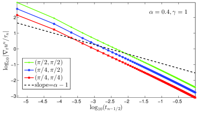
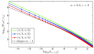
Figure 1: The log-log plot of difference quotient $\nabla_{\tau}u_{h}^{n}/\tau_{n}$ versus the time for Example 1 ($\alpha=0.4$) with two grading parameters $\gamma=1$ (left) and $\gamma=3$ (right).

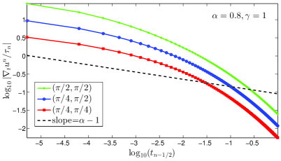
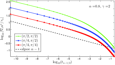
Figure 2: The log-log plot of difference quotient $\nabla_{\tau}u_{h}^{n}/\tau_{n}$ versus the time for Example 1 ($\alpha=0.8$) with two grading parameters $\gamma=1$ (left) and $\gamma=2$ (right).

In our simulations, the spatial domain $\Omega$ is divided uniformly into $M$ parts in each direction $(M_{1}=M_{2}=M)$ and the time interval $[0,T]$ is divided into two parts $[0,T_{0}]$ and $[T_{0},T]$ with total $N_{T}$ subintervals. According to the suggestion in [15], the graded mesh $t_{k}=T_{0}\left(k/N\right)^{\gamma}$ is applied in the cell $[0,T_{0}]$ and the uniform mesh with time step size $\tau\geq\tau_{N}$ is used over the remainder interval. Given certain final time $T$ and a proper number $N_{T}$, here we would take $T_{0}=\min\{1/\gamma,T\}$, $N=\big{\lceil}\frac{N_{T}}{T+1-\gamma^{-1}}\big{\rceil}$ such that $\tau=\frac{T-T_{0}}{N_{T}-N}\geq\frac{T+1-\gamma^{-1}}{N_{T}}\geq N^{-1}\geq\tau_{N}.$ Always, the absolute tolerance error of SOE approximation is set to $\epsilon=10^{-12}$ such that the two-level L1 formula (2.5a) is comparable with the L1 formula (2.2) in time accuracy.

In Example 1, we investigate the asymptotic behavior of solution near $t=0$ and the computational efficiency of the linearized method (2.6). Setting $M=100$, $T=1/\gamma$ and $N_{T}=100$, Figures 1-2 depict, in log-log plot, the numerical behaviors of first-order difference quotient $\nabla_{\tau}u_{h}^{n}/\tau_{n}$ at three spatial points near the initial time for different fractional orders and grading parameters. Observations suggest that $\log\left|u_{t}(\boldsymbol{x},t)\right|\approx C_{u}(\boldsymbol{x})+(\alpha-1)\log t$ as $t\rightarrow 0$, and the solution is weakly singular near the initial time. Compared with the uniform grid, the graded mesh always concentrates much more points in the initial time layer and provides better resolution for the initial singularity.

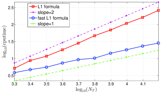
Figure 3: The log-log plot of CPU time versus the total number $N_{T}$ of time levels for the linearized method in solving Example 1 with two different formulas of Caputo derivative.

To see the effectiveness of our linearized method (2.6), we also consider another linearized method by replacing the two-level fast L1 formula $(D^{\alpha}_{f}u_{h})^{n}$ with the nonuniform L1 formula $(D^{\alpha}_{\tau}u_{h})^{n}$ defined in (2.2). Setting $\alpha=0.5$, $\gamma=2$, and $M=50$, the two schemes are run for Example 1 to the final time $T=50$ with different total numbers $N_{T}$. Figure 3 shows the CPU time in seconds for both linearized procedures versus the total number $N_{T}$ of subintervals. We observe that the proposed method has almost linear complexity in $N_{T}$ and is much faster than the direct scheme using traditional L1 formula.

Since the spatial error $O(h^{2})$ is standard, the time accuracy due to the numerical approximations of Caputo derivative and nonlinear reaction is examined in Example 2 with $T=1$. The maximum norm error $e(N,M)=\max_{1\leqslant l\leqslant N}\big{\|}U(t_{l})-u^{l}\big{\|}_{\infty}.$ To test the sharpness of our error estimate, we consider three different scenarios, respectively, in Tables 5.1-5.3:

Table 5.1

: $\sigma=2-\alpha$ and $\gamma=1$ with fractional orders $\alpha=0.4$, $0.6$ and $0.8$.

Table 5.2

: $\alpha=0.4$ and $\sigma=0.4$ with grid parameters $\gamma=1$, $\frac{3}{4}\gamma_{\texttt{opt}}$, $\gamma_{\texttt{opt}}$ and $\frac{5}{4}\gamma_{\texttt{opt}}$.

Table 5.3

: $\alpha=0.4$ and $\sigma=0.8$ with grid parameters $\gamma=1$, $\frac{3}{4}\gamma_{\texttt{opt}}$, $\gamma_{\texttt{opt}}$ and $\frac{5}{4}\gamma_{\texttt{opt}}$.

Table 5.1  Numerical temporal accuracy for $\sigma=2-\alpha$ and $\gamma=1$   $N$ $\alpha=0.4$,$\sigma=1.6$ $\alpha=0.6$,$\sigma=1.4$ $\alpha=0.8$,$\sigma=1.2$ $e(N)$ Order $e(N)$ Order $e(N)$ Order 50 5.69e-04 – 1.14e-03 – 2.57e-03 – 100 1.57e-04 1.86 4.65e-04 1.30 1.23e-03 1.07 200 4.40e-05 1.84 1.88e-04 1.31 5.80e-04 1.08 400 1.45e-05 1.60 7.51e-05 1.32 2.71e-04 1.10 800 5.02e-06 1.53 2.98e-05 1.34 1.25e-04 1.12 $\min\{\gamma\sigma,2-\alpha\}$ 1.60 1.40 1.20  

Tables 5.1 lists the solution errors, for $\sigma=2-\alpha$, on the gradually refined grids with the coarsest grid of $N=50$. Numerical data indicates that the optimal time order is of about $O(\tau^{2-\alpha})$, which dominates the spatial error $O(h^{2})$. Always, we take $M=N$ in Tables 5.1-5.3 such that $e(N,M)\approx e(N)$. The experimental rate (listed as Order in tables) of convergence is estimated by observing that $e(N)\approx C_{u}\tau^{\beta}$ and then $\beta\approx\log_{2}\left[{e(N)}/{e(2N)}\right].$

Table 5.2  Numerical temporal accuracy for $\alpha=0.4$, $\sigma=0.4$ and $\gamma_{\texttt{opt}}=4$   $N$ $\gamma=1$ $\gamma=3$ $\gamma=4$ $\gamma=5$ $e(N)$ Order $e(N)$ Order $e(N)$ Order $e(N)$ Order 50 5.47e-02 – 3.82e-03 – 1.65e-03 – 1.32e-03 – 100 4.64e-02 0.24 1.68e-03 1.18 5.78e-04 1.52 4.60e-04 1.52 200 3.78e-02 0.30 7.36e-04 1.19 1.99e-04 1.54 1.58e-04 1.54 400 3.00e-02 0.33 3.21e-04 1.20 6.78e-05 1.55 5.37e-05 1.56 800 2.34e-02 0.36 1.40e-04 1.20 2.30e-05 1.56 1.81e-05 1.57 $\min\{\gamma\sigma,2-\alpha\}$ 0.40 1.20 1.60 1.60  

Table 5.3  Numerical temporal accuracy for $\alpha=0.4$, $\sigma=0.8$ and $\gamma_{\texttt{opt}}=2$   $N$ $\gamma=1$ $\gamma=3/2$ $\gamma=2$ $\gamma=5/2$ $e(N)$ Order $e(N)$ Order $e(N)$ Order $e(N)$ Order 50 3.46e-03 – 8.72e-04 – 5.80e-04 – 7.52e-04 – 100 2.20e-03 0.65 3.93e-04 1.15 1.39e-04 2.08 1.77e-04 2.08 200 1.34e-03 0.72 1.75e-04 1.17 3.80e-05 1.87 4.06e-05 2.13 400 7.95e-04 0.75 7.70e-05 1.18 1.32e-05 1.53 8.88e-06 2.19 600 5.83e-04 0.77 4.76e-05 1.19 7.06e-06 1.54 4.22e-06 1.55 800 4.67e-04 0.77 3.38e-05 1.19 4.52e-06 1.55 2.70e-06 1.55 $\min\{\gamma\sigma,2-\alpha\}$ 0.80 1.20 1.60 1.60  

Numerical results in Tables 5.2-5.3 (with $\alpha=0.4$ and $\sigma<2-\alpha$) support the predicted time accuracy in Theorem 4.2 on the smoothly graded mesh $t_{k}=T(k/N)^{\gamma}$. In the case of a uniform mesh $(\gamma=1)$, the solution is accurate of order $O(\tau^{\sigma})$, and the nonuniform meshes improve the numerical precision and convergence rate of solution evidently. The optimal time accuracy $O(\tau^{2-\alpha})$ is observed when the grid parameter $\gamma\geq(2-\alpha)/\sigma$.

Appendix A Proof of Lemma 4.1

Proof  Consider $F(\psi)=\psi$ firstly. It is easy to check that, at point $\boldsymbol{x}_{h}=(x_{i},y_{j})\in\Omega_{h}$,

$$\delta_{x}^{2}(\psi_{ij}v_{ij})=\psi_{ij}\big{(}\delta_{x}^{2}v_{ij}\big{)}+\delta_{x}\psi_{i-\frac{1}{2},j}\big{(}\delta_{x}v_{i-\frac{1}{2},j}\big{)}+\delta_{x}\psi_{i+\frac{1}{2},j}\big{(}\delta_{x}v_{i+\frac{1}{2},j}\big{)}+v_{ij}\big{(}\delta_{x}^{2}\psi_{ij}\big{)}\,,$$

so that $\|\delta_{x}^{2}(\psi v)\|\leqslant C_{0}\left(\|v\|+\|\delta_{x}v\|+\|\delta_{x}^{2}v\|\right)$. Similarly, $\|\delta_{y}^{2}(\psi v)\|\leqslant C_{0}\left(\|v\|+\|\delta_{y}v\|+\|\delta_{y}^{2}v\|\right).$ Moreover, one has $\|\delta_{y}\delta_{x}(\psi v)\|\leqslant C_{0}\left(\|v\|+\|\delta_{x}v\|+\|\delta_{y}v\|+\|\delta_{y}\delta_{x}v\|\right)$, due to the fact

$$\delta_{y}\delta_{x}(\psi_{i-\frac{1}{2},j-\frac{1}{2}}v_{i-\frac{1}{2},j-\frac{1}{2}})= \,\psi_{i-\frac{1}{2},j-\frac{1}{2}}\big{(}\delta_{y}\delta_{x}v_{i-\frac{1}{2},j-\frac{1}{2}}\big{)}+\delta_{y}\psi_{i-\frac{1}{2},j-\frac{1}{2}}\big{(}\delta_{x}v_{i-\frac{1}{2},j-\frac{1}{2}}\big{)}$$

$$\,+\delta_{x}\psi_{i-\frac{1}{2},j-\frac{1}{2}}\big{(}\delta_{y}v_{i-\frac{1}{2},j-\frac{1}{2}}\big{)}+\big{(}\delta_{y}\delta_{x}\psi_{i-\frac{1}{2},j-\frac{1}{2}}\big{)}v_{i-\frac{1}{2},j-\frac{1}{2}}\,.$$

Noticing that $\left\|\Delta_{h}v\right\|^{2}=\|\delta_{x}^{2}v\|^{2}+2\|\delta_{x}\delta_{y}v\|^{2}+\|\delta_{y}^{2}v\|^{2}$, we apply the embedding inequalities in (2.1) to obtain, also see [12, Lemma 2.2],

$$\left\|\Delta_{h}(\psi v)\right\|\leqslant C_{u}\left(\left\|v\right\|+\left\|\Delta_{h}v\right\|\right)\leqslant C_{F}\left\|\Delta_{h}v\right\|,$$

where the constant $C_{F}$ is dependent on $C_{0}$ and $C_{\Omega}$. For the general case $F\in C^{2}(\mathbb{R})$, one has

$$\delta_{x}^{2}\big{[}F(\psi_{ij})v_{ij}\big{]}= \,F(\psi_{ij})\big{(}\delta_{x}^{2}v_{ij}\big{)}+\delta_{x}F(\psi_{i-\frac{1}{2},j})\big{(}\delta_{x}v_{i-\frac{1}{2},j}\big{)}$$

$$\,+\delta_{x}F(\psi_{i+\frac{1}{2},j})\big{(}\delta_{x}v_{i+\frac{1}{2},j}\big{)}+v_{ij}\big{[}\delta_{x}^{2}F(\psi_{ij})\big{]}\,.$$

The formula of Taylor expansion with integral remainder gives

$$\delta_{x}F(\psi_{i-\frac{1}{2},j})= \,\big{(}F(\psi_{ij})-F(\psi_{i-1,j})\big{)}/h_{1}=\delta_{x}\psi_{i-\frac{1}{2},j}\int_{0}^{1}F^{\prime}\big{(}s\psi_{ij}+(1-s)\psi_{i-1,j}\big{)}\,\mathrm{d}{s}\,,$$

$$\delta_{x}^{2}F(\psi_{ij})= \,\big{(}\delta_{x}^{2}\psi_{ij}\big{)}F^{\prime}(\psi_{ij})+\big{(}\delta_{x}\psi_{i-\frac{1}{2},j}\big{)}^{2}\int_{0}^{1}F^{\prime\prime}\big{(}s\psi_{ij}+(1-s)\psi_{i-1,j}\big{)}(1-s)\,\mathrm{d}{s}$$

$$\,\hskip 68.28644pt+\big{(}\delta_{x}\psi_{i+\frac{1}{2},j}\big{)}^{2}\int_{0}^{1}F^{\prime\prime}\big{(}s\psi_{ij}+(1-s)\psi_{i+1,j}\big{)}(1-s)\,\mathrm{d}{s}\,,$$

such that $\|\delta_{x}F(\psi)\|\leqslant C_{F}$ and $\|\delta_{x}^{2}F(\psi)\|\leqslant C_{F}\,$. Therefore, simple calculations arrive at

$$\|\delta_{x}^{2}\left[F(\psi)v)\right]\|\leqslant C_{F}\left(\|v\|+\|\delta_{x}v\|+\|\delta_{x}^{2}v\|\right)\,.$$

By presenting similar arguments as those in the above simple case, it is straightforward to get claimed estimate and complete the proof.

References

- [1] D. Baffet and J.S. Hesthaven, A kernel compression scheme for fractional differential equations, SIAM J. Numer. Anal., 55(2) (2017), 496-520.
- [2] H. Brunner, Collocation methods for Volterra integral and related functional differential equations, 15 (2004), Cambridge University Press, Cambridge.
- [3] H. Brunner, L. Ling and M. Yamamoto, Numerical simulations of 2D fractional subdiffusion problems, J. Comput. Phys., 229 (2010), 6613-6622.
- [4] S. Jiang, J. Zhang, Q. Zhang and Z. Zhang, Fast evaluation of the Caputo fractional derivative and its applications to fractional diffusion equations, Commun. Comput. Phys., 21(3) (2017), 650-678.
- [5] B. Jin, B. Li and Z. Zhou, Numerical analysis of nonlinear subdiffusion equations, SIAM J. Numer. Anal., 56(1) (2018), 1-23.
- [6] R. Hilfer, ed., Applications of fractional calculus in physics, World Scientific, Singapore, 2000.
- [7] B. Li and W. Sun, Error analysis of linearized semi-implicit Galerkin finite elementmethods for nonlinear parabolic equations, Int. J. Numer. Anal. Model., 10 (2013), 622-633.
- [8] B. Li and W. Sun, Unconditional convergence and optimal error estimates of a Galerkin-mixed FEM for incompressible miscible flow in porous media, SIAM J. Numer. Anal., 51 (2013), 1959-1977.
- [9] B. Li, J. Wang and W. Sun, The stability and convergence of fully discrete Galerkin FEMs for porous medium flows, Commun. Comput. Phys., 15 (2014), 1141-1158.
- [10] C. Li, Q. Yi and A. Chen, Finite difference methods with non-uniform meshes for nonlinear fractional differential equations, J. Comput. Phys., 316 (2016), 614-631.
- [11] J. Li, A fast time stepping method for evaluating fractional integrals, SIAM J. Sci. Comput., 31 (2010), 4696-4714.
- [12] H.-L. Liao, Z. Z. Sun and H. S. Shi, Error estimate of fourth-order compact scheme for solving linear Schrödinger equations, SIAM. J. Numer. Anal., 47(6) (2010), 4381-4401.
- [13] H.-L. Liao, Z. Z. Sun and H. S. Shi, Maximum norm error analysis of explicit schemes for two-dimensional nonlinear Schrödinger equations (in Chinese), Science China Mathematics, 40(9) (2010), 827-842.
- [14] H.-L. Liao and Z. Z. Sun, Maximum norm error bounds of ADI and compact ADI methods for solving parabolic equations, Numer. Methods PDEs, 26 (2010), 37-60.
- [15] H.-L. Liao, D. Li and J. Zhang, Sharp error estimate of nonuniform L1 formula for linear reaction-subdiffusion equations, To appear in SIAM J. Numer. Anal., 2018.
- [16] H.-L. Liao, W. McLean and J. Zhang, A discrete Grönwall inequality with application to numerical schemes for reaction-subdiffusion problems, 2018, Preprint, DOI:10.13140/RG.2.2.34292.86408.
- [17] K. Mustapha and H. Mustapha, A second-order accurate numerical method for a semilinear integro-differential equation with a weakly singular kernel, IMA J. Numer. Anal., 30(2) (2010), 555-578.
- [18] I. Podlubny, Fractional differential equations, Academic Press, New York, 1999.
- [19] M. Stynes, E. O’Riordan and J. L. Gracia, Error analysis of a finite difference method on graded meshes for a time-fractional diffusion equation, SIAM J. Numer. Anal., 55(2) (2017), 1057-1079.
- [20] Q. Xu, J.S. Hesthaven and F. Chen, A parareal method for time-fractional differential equations, J. Comp. Phys., 293(C) (2015), 173-183.
- [21] Y. Yan, Z. Z. Sun and J. Zhang, Fast evaluation of the Caputo fractional derivative and its applications to fractional diffusion equations: a second-order scheme, Commun. Comput. Phys., 22 (2017), 1028-1048.
- [22] Y.N. Zhang, Z.Z. Sun and H.-L. Liao, Finite difference methods for the time fractional diffusion equation on nonuniform meshes, J. Comput. Phys., 265 (2014), 195-210.