Universal dynamics of zero-momentum to plane-wave transition in spin-orbit coupled Bose-Einstein condensates
Abstract
We investigate the universal spatiotemporal dynamics in spin-orbit coupled Bose-Einstein condensates which are driven from the zero-momentum phase to the plane-wave phase. The excitation spectrum reveals that, at the critical point, the Landau critical velocity vanishes and the correlation length diverges. Therefore, according to the Kibble-Zurek mechanism, spatial domains will spontaneously appear in such a quench through the critical point. By simulating the real-time dynamics, we numerically extract the static correlation length critical exponent and the dynamic critical exponent from the scalings of the temporal bifurcation delay and the spatial domain number. The numerical scalings consist well with the analytical ones obtained by analyzing the excitation spectrum.
Keywords: Bose-Einstein condensation, quantum criticality, quantum phase transitions, quantum quenches
1 Introduction
The critical behavior near a continuous phase transition has been explored in many areas of physics, including cosmology, particle physics and condensed matter. When a system is driven across a continuous phase transition point, both the relaxation time and correlation length diverge at the critical point, so that the time-evolution cannot be adiabatic no matter how slow the quench is. Therefore, for a quench with finite quench rate, the system will go out of equilibrium near the critical point and defects spontaneously form. The Kibble-Zurek mechanism (KZM) [1, 2, 3, 4] provides a general theory for understanding the non-equilibrium dynamics crossing the critical point and predicts universal scaling laws of the defect density with respect to the quench rate. The KZM have been found in various systems, such as the early universe [1], superfluid helium [2], liquid crystal[5] and ion crystal[6, 7]. Recently, due to the extraordinary degree of flexibility and high controllability, atomic Bose-Einstein condensates (BECs) becomes an excellent candidates for exploring the KZM, in both thermodynamic [8, 9, 10, 11, 12, 13, 14, 15] and quantum phase transitions [16, 17, 18, 19, 20, 21, 22, 23, 24, 25, 26, 27, 28].
In recent years, one remarkable advance in cold atom research is the realization of spin-orbit (SO) coupling. In the pioneering experiments, the SO coupling is created with two spin states of coupled by two counter propagating Raman lasers [29]. Due to the competition of the SO coupling and the atom-atom interactions, various novel superfluid phases emerge. The ground-state phase diagram is predicted to include a stripe phase, a plane-wave phase and a zero-momentum phase [30, 31]. A great amount of experimental and theoretical efforts have been dedicated to study the ground-state properties and static phase transitions [32, 33, 34, 35, 36, 37]. The phase transition dynamics and the critical scaling behavior, however, have rarely been explored. In fact, the high tunability of Raman coupling parameters makes SO coupled BECs an ideal platform to test the KZM. Taking advantage of the simplicity of experimental setup and the developed techniques, we suppose that SO coupled two-component BECs could be a good choice to explore the critical behavior.
In this paper, we investigate the KZM in SO coupled two-component BECs by both analyzing the Bogoliubov excitations and the population dynamics during the phase transition. We find spatial domains form spontaneously after quenching through critical point due to the vanish of Landau critical velocity and the divergence of correlation length. The KZ scalings can be extracted from the excitation spectrum and the scaling of Landau critical velocity. On the other hand, by simulating the real-time dynamics, we find that the average bifurcation delay and average domain number follow universal scaling laws given by the KZM. The critical exponents derived from the numerical results consist well with the analytical ones.
The paper is organized as follows. In Sec. II, we describe the model and ground-state phase diagram. We also give a brief introduction to the KZM. In Sec. III, we calculate the Bogoliubov excitations to study the Landau critical velocity and the critical scalings. In Sec. IV, we show how to extract the critical exponents from the real-time dynamics. In Sec. V, we summarize our results and briefly discuss the experimental feasibility.
2 Zero-momentum to plane-wave transition and Kibble-Zurek mechanism
We consider a pseudo-spin-1/2 atomic Bose gas with Raman process induced SO coupling along x-direction [29]. For simplicity, we restrict our discussion to an elongated system where the dynamics are confined to the x-direction and assume that the system remains in the ground-states in the transverse directions. The single particle effective Hamiltonian in the pseudo-spin-1/2 basis can be written as (set ):
| (1) |
Here, is the recoil momentum of Raman coupling, is the Raman coupling strength, is the Raman detuning, and are Pauli matrices. In the following, energy is conveniently measured in units of the recoil energy .
Considering also the atom-atom interactions, the mean-field (MF) energy functional of the system can be expressed as:
| (5) | |||
| (6) |
Here, and are the intra-species interaction strength and is the inter-species interaction strength, which are determined by the intra-species and inter-species -wave scattering lengths respectively. In the following parts, we consider only the spin-symmetry interaction and the resonance case for simplification. Therefore the interaction energy can be rewritten as:
| (7) |
in which and are the densities for the two spin components.
To obtain the ground-state wave-function , one can utilize the variational method and adopt the variational ansatz [31]:
| (14) |
in which is the average atom density with and being the total atom number and the size of the system in x-direction, and , and are the variational parameters. The normalization condition indicates . By inserting the condensates wave-function (14) into the energy functional (2) and minimizing the energy with respect to the variational parameters, one can obtain the ground-state for given and interaction strength and . The ground-state phase diagram has been discussed in the work by Li et al. [31] and we just give a brief summary here.
(I) When is relatively small, the energy functional (2) has two degenerate minima at and the condensate wave-function is the superposition of these two quasimomentum components, namely and in the ansatz (14). Therefore the densities of both spin components have spatial modulation. This is named as a stripe condensate.
(II) As increases, the density modulation in the stripe phase increases and the density-density term in the interaction energy (7) cost more and more energy. When exceeds a critical value , the minimization of energy functional (2) gives either or . The condensate wave-function has a single quasimomentum component, which is named as a plane-wave (PW) condensate.
(III) If further increases and exceeds another critical value , the two minima at will emerge into a single minimum at . Then the condensate wave-function is a plane-wave with zero quasimomentum (ZM), which is named as a ZM condensate.
(IV) If the average atom density exceeds a critical value , the stripe condensate always have a lower energy than the PW condensate. Therefore, there will be a direct transition from the stripe phase to the ZM phase when .
Here we concentrate on the transition from the ZM phase to the PW phase, which is a second-order phase transition since a single minimum in the energy dispersion splits into two minima with the quasimomentum changing continuously. The critical coupling strength for the transition from the ZM phase to the PW phase is
| (15) |
in which ; in the PW phase the two minima locate at
| (16) |
and the variational parameter in the ground-state wave-function (14) is
| (17) |
In addition, to characterize different phases, we can define the spin polarization as:
| (18) |
in which . The ZM condensate has a zero while PW condensate has a nonzero .
In the SO coupled BECs, by adjusting the coupling strength from an initial value to a final value , the system is driven across the critical point of the continuous phase transition; see the inset of figure 1. The corresponding nonequilibrium dynamics are expected to show a universal scaling behavior according to the KZM. It is convenient to define the dimensionless distance from the critical point as
| (19) |
We linearly quench the Raman coupling strength , so that the dimensionless distance varies linearly near the critical point as
| (20) |
in which is the quench time. When , the correlation length and the relaxation time of the system diverge as [3]:
| (21) |
where and are the critical exponents.
According to the KZM, the evolution of the system during the quench can be divided into three stages decided by two characteristic time scales. One time scale is the relaxation time , which characterizes how fast the system follows the ground-state of its instantaneous Hamiltonian. The other time scale is the transition time , which describes how fast the time-dependent parameter changes. Initially, when the system is far away from the critical point, the relaxation time is shorter than the transition time so that the system can follow the instantaneous ground-state adiabaticlly. Because of the divergence of near the critical point, the transition from the adiabatic stage to the impulse stage happens when the two time scales become comparable, which defines the freezing time according to
| (22) |
In the impulse stage, the system becomes effectively frozen and stays in the instantaneous ground-state of the time . When the two time scales become comparable again at , which is called freeze-out time, the adiabatic evolution of the state restarts. At the freeze-out time, the dimensionless distance and the correlation length both have power-law scalings as a function of the quench time :
| (23) |
After the impulse-adiabatic transition, the system locates in the PW phase, which has two degenerate ground-states with different nonzero quasimomenta. Therefore the system choose the state randomly in the space and domains appear. Since the domains at a distance larger than the correlation length form independently, the average domain number at scales as:
| (24) |
where is the number of space dimensions.
In the following, we will explore the universal critical dynamics and derive the critical exponents and through two complementary approaches, by analyzing the Bogoliubov excitation spectrum and by performing numerical simulation of the real-time dynamics.
3 Spontaneous superfluidity breakdown near the critical point
In this section, we investigate the universal scaling by analyzing the spontaneous breakdown of superfluidity. According to the Landau criterion, if the superfluid velocity is less than the Landau critical velocity, the elementary excitations is prohibited due to the conservation of energy and momentum. However, around a continuous phase transition, the Landau critical velocity vanishes and elementary excitations appear spontaneously. We will show that the scaling exponents can be extracted from the excitation spectrum and the Landau critical velocity.
Firstly, we perform a Bogoliubov analysis to obtain the excitation modes over the MF ground-states. By minimizing the MF energy functional (2) with respect to the wave-functions , one obtains two-component time-dependent Gross-Pitaevskii equations (GPEs), which describe the dynamics of the system. The GPEs read as:
In the PW and ZM phase, the condensate wave-function can be expanded as:
| (26) |
in which is the chemical potential and are the wave-function amplitudes. In the PW phase, the ground-state with quasimomentum has wave-function amplitudes while the ground-state with quasimomentum has wave-function amplitudes . For simplicity, we choose the ground-state with the quasimomentum in calculating the excitation spectrum for the PW phase. In the ZM phase, the ground-state has . To determine the Bogoliubov excitation spectrum, we consider small perturbations around the ground-state
| (27) |
Inserting equation (27) into the equations (3), one obtains the linearized equations for the perturbations:
| (28) | |||||
| (29) | |||||
The perturbations can be written in the form
| (30) |
in which is the excitation momentum, is the excitation frequency, and and are the complex amplitudes. Substituting equation (30) to the linearized equations (28) and comparing the coefficients for the terms of and , one can obtain the Bogoliubov-de-Gennes (BdG) equations:
| (31) |
in which , and
| (32) |
with
| (35) | |||
| (38) | |||
| (41) |
Then the excitation spectrum can be obtained by diagonalizing the matrix . Three typical excitation spectra for the system in the PW phase, the ZM phase and the critical point are shown in figure 1.
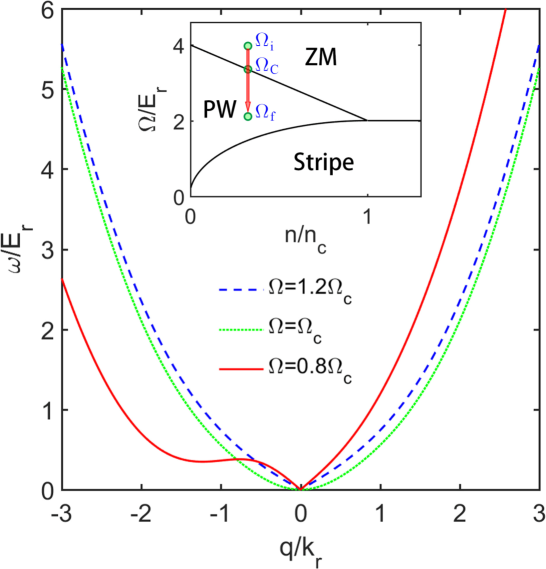
From figure 1, we see that the excitation spectra exhibit phonon modes with linear dispersions in long wavelength limit for both PW phase and ZM phase, namely for , and for , where () is the sound velocity in the negative (positive) x-direction. The phonon modes in the excitation spectrum are significant features of superfluidity. Interestingly, at the critical point between the PW and ZM phases, softening of the phonon modes is observed and the elementary excitations exhibit a dependence (see the dotted line in figure 1), which is due to the divergency of the effective mass associated with the single particle spectrum at the critical point [38]. Since as at a continuous phase transition [39, 40, 41], we have the dynamical critical exponent .
The Landau critical velocity
| (42) |
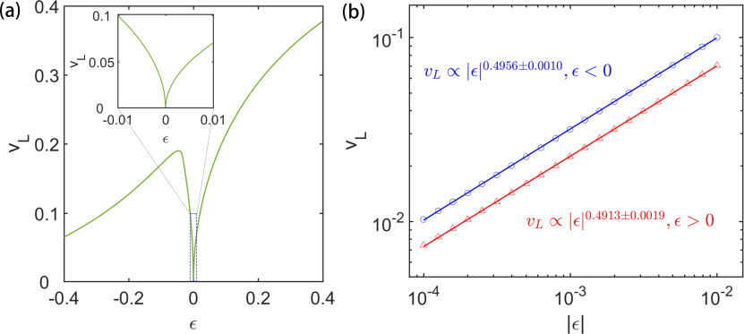
for different can be directly extracted from the excitation spectrum. As illustrated in figure 2a, the Landau critical velocity vanishes at the critical point , which is due to the softening of the phonon modes, namely as . Therefore, elementary excitations can appear spontaneously around the phase transition. In the ZM phase, the Landau critical velocity equals with the sound velocity and increase monotonously with increasing . Remarkably, we observe a nonmonotonic behavior of with increasing in the PW phase, which originates from the roton structure in the excitation spectrum [38, 42]; see the solid line in figure 1. In the small regime of the PW phase, is still equal to the smaller sound velocity of . However, due to the appearance of the roton structure, in the larger regime is no longer equals with the sound velocity but decided by the roton minimum. Since the energy of the roton minimum decrease with an increasing , will be suppressed more and more strongly as increases.
Generally speaking, the correlation length is defined by the equality between the kinetic energy per particle and the interaction energy per particle . However, the Landau critical velocity provides another general definition of the correlation length according to , which is consistent with the usual definition [43]. Therefore, the Landau critical velocity should have a power-law scaling behavior around the critical point as:
| (43) |
In figure 2b, we plot the for different near the critical point in a log-log coordinate. It shows clearly that has a power-law dependence on , which can be expressed by . Through linear fitting, we find and for the PW and ZM phases respectively. This indicates that the static correlation length critical exponent .
4 Time-evolution dynamics across the critical point
In this section, we show how to obtain the Kibble-Zurek scalings from the real-time dynamics. We perform numerical simulations of spontaneous magnetization and domain formation based on the GPEs (3). Starting with the ZM phase, we linearly change the Raman coupling strength to drive the system across the critical point between ZM and PW phases according to
| (44) |
In our simulation, we adopt various quench times over two orders of magnitude and we perform 100 runs of simulations for each . On the other hand, since the quantum fluctuations that trigger the growth of magnetization are ignored in the MF approximation [17], we introduce appropriate noise to the initial state so that the dynamics of spontaneous magnetization can be studied by the MF theory.
After the Raman coupling strength sweeping through the bifurcation point of the quantum phase transition, the BECs manifest delayed development of spin fluctuation. To determine the freeze-out time in each single run, one can utilize fluctuations of the spin polarization
| (45) |
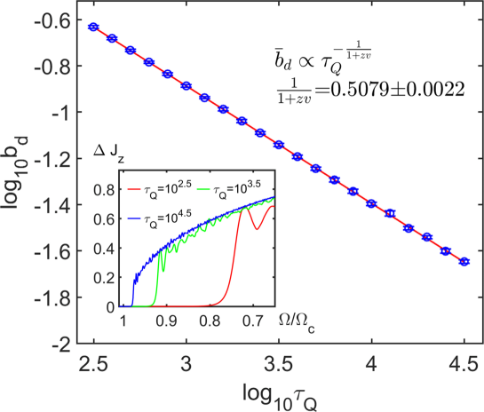
Since the critical exponents and are insensitive to the choice of the thresholds [18], we adopt the threshhold in our numerical results. We have also checked that the same conclusions can be obtained for other thresholds between to . In figure 3, we show the bifurcation delay for different quench time . It is clear that the growth of spin fluctuations lags the phase transition point by an amount of and the system stays frozen for a larger bifurcation delay for smaller quench time; see the inset of figure 3. Such bifurcation delay has also been reported in laser pumped BECs [44]. In figure 3, it is illustrated that the average bifurcation delay fits well to a power-law scaling with respect to the quench time , which yields an exponent . Since , we obtain according to (23).
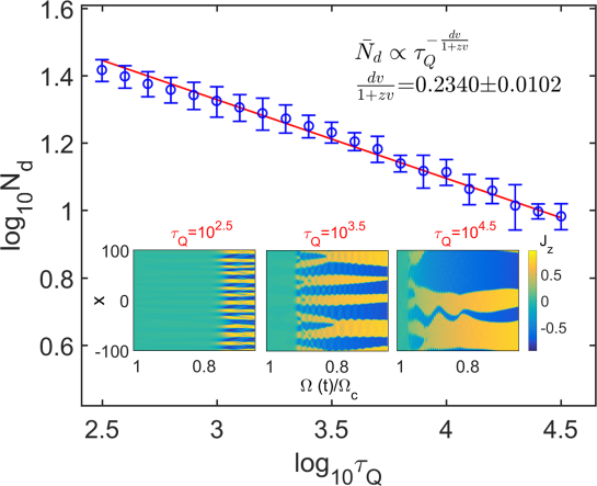
In order to extract the critical exponents, we also analysis the universal scaling of domain number versus quench time . Typical examples of domain-formation dynamics for different quench times are illustrated in the insets of figure 4. One can see that ferromagnetic domains form after the system crossing the phase transition point and the average domain size increase with the quench time. In each run, we count the domain number by identifying the number of zero crossings of at the unfreezing time . The domain numbers for different are summarized in figure 4. We observe that the average domain number follows a power-law scaling as expected from the KZM, which gives the scaling exponent . We have checked that similar scaling of the average domain numbers can be obtained for other thresholds of between to .
Finally, combining the scaling exponents of the average bifurcation delay and the average domain number with respect to , we obtain the critical exponents and , which consist with the analytical exponents obtained in Sec. III and agree well with the MF exponents and .
5 Conclusions and discussions
In summary, we have investigated the universal spatiotemporal dynamics across a second-order phase transition point in SO coupled two-component BECs. Due to the divergence of correlation length and relaxation time at the critical point, spatial domains form in the phase transition dynamics according to the KZM. We analyze the Bogoliubov excitation spectrum and find the Landau critical velocity vanishes at the phase transition point, which results in the spontaneous appearance of the elementary excitations. We extract the critical exponents from the excitation spectrum and the scaling of the Landau critical velocity around the critical point. On the other hand, we numerically find that the average bifurcation delay and the average domain number after the system crossing the critical point follow a universal scaling law as expected by the KZM. We also extract the critical exponents from the numerical scalings. The critical exponents given by the two methods consist with each other.
Based upon current available techniques for SO coupled BECs, it is possible to probing the above KZ scalings. The SO coupling can be synthesized in two-component BECs with two counter propagating Raman lasers [29]. The plane-wave phase and the zero-momentum phases have been observed in present experiments [35] and the high tunability of the Raman coupling parameters make the quenching across the phase transition point possible. The KZ scalings can then be obtained by measuring the bifurcation delay and the size of ferromagnetic domains for different quench rates via the time-of-flight [24].
References
References
- [1] Kibble T W B 1976 Topology of cosmic domains and strings J. Phys. Math. Gen. 9 1387.
- [2] Zurek W H 1985 Cosmological experiments in superfluid helium? Nature 317 505.
- [3] Dziarmaga J 2010 Dynamics of a quantum phase transition and relaxation to a steady state Adv. Phys. 59 1063.
- [4] Campo A and Zurek W H 2014 Universality of phase transition dynamics: Topological defects from symmetry breaking Int. J. Mod. Phys. A 29 1430018.
- [5] Nikkhou M, Skarabot M, Copar S, Ravnik M, Zumer S and Musevic I 2015 Light-controlled topological charge in a nematic liquid crystal Nat. Phys. 11 183.
- [6] Ulm S, et al. 2013 Observation of the Kibble-Zurek scaling law for defect formation in ion crystals Nat. Commun. 4 2290.
- [7] Pyka K, et al. 2013 Topological defect formation and spontaneous symmetry breaking in ion Coulomb crystals Nat. Commun. 4 2291.
- [8] Damski B and Zurek W H 2010 Soliton creation during a Bose-Einstein condensation Phys. Rev. Lett. 104 160404.
- [9] Das A, Sabbatini J and Zurek W H 2012 Winding up superfluid in a torus via Bose-Einstein condensation Sci. Rep. 2 352.
- [10] Donner T, Ritter S, Bourdel T, Öttl A, Köhl M and Esslinger T 2007 Critical behavior of a trapped interacting Bose gas Science 315 1556.
- [11] Lamporesi G, Donadello S, Serafini S, Dalfovo F and Ferrari G 2013 Spontaneous creation of Kibble-Zurek solitons in a Bose-Einstein condensate Nat. Phys. 9 656.
- [12] Navon N, Gaunt A L, Smith R P and Hadzibabic Z 2015 Critical dynamics of spontaneous symmetry breaking in a homogeneous Bose gas Science 347 167.
- [13] Su S, Gou S, Bradley A, Fialko O and Brand J 2013 Kibble-Zurek scaling and its breakdown for spontaneous generation of Josephson vortices in Bose-Einstein condensates Phys. Rev. Lett. 110 215302.
- [14] Weiler C N, Neely T W, Scherer D R, Bradley A S, Davis M J and Anderson B P 2008 Spontaneous vortices in the formation of Bose-Einstein condensates Nature 455 948.
- [15] Witkowska E, Deuar P, Gajda M and Rzazewski K 2011 Solitons as the early stage of quasicondensate formation during evaporative cooling Phys. Rev. Lett. 106 135301.
- [16] Uhlmann M, Schützhold R and Fischer U R 2007 Vortex quantum creation and winding number scaling in a quenched spinor Bose gas Phys. Rev. Lett. 99 120407.
- [17] Saito H, Kawaguchi Y and Ueda M 2007 Kibble-Zurek mechanism in a quenched ferromagnetic Bose-Einstein condensate Phys. Rev. A 76 043613.
- [18] Damski B and Zurek W H 2007 Dynamics of a quantum phase transition in a ferromagnetic Bose-Einstein condensate Phys. Rev. Lett. 99 130402.
- [19] Dziarmaga J, Meisner J and Zurek W H 2008 Winding up of the wave-function phase by an insulator-to-superfluid transition in a ring of coupled Bose-Einstein condensates Phys. Rev. Lett. 101 115701.
- [20] Lee C 2009 Universality and anomalous mean-field breakdown of symmetry-breaking transitions in a coupled two-component Bose-Einstein condensate Phys. Rev. Lett. 102 070401.
- [21] Chen D, White M, Borries C and DeMarco B 2011 Quantum quench of an atomic Mott insulator Phys. Rev. Lett. 106 235304.
- [22] Sabbatini J, Zurek W H and Davis M J 2011 Phase separation and pattern formation in a binary Bose-Einstein condensate Phys. Rev. Lett. 107 230402.
- [23] Anquez M, Robbins B A, Bharath H M, Boguslawski M, Hoang T M and Chapman M S 2016 Quantum Kibble-Zurek mechanism in a spin-1 Bose-Einstein condensate Phys. Rev. Lett. 116 155301.
- [24] Clark L W, Feng L, Chin C 2016 Universal space-time scaling symmetry in the dynamics of bosons across a quantum phase transition Science 354 606.
- [25] Xu J, Wu S, Qin X, Huang J, Ke Y, Zhong H and Lee C 2016 Kibble-Zurek dynamics in an array of coupled binary Bose condensates EPL 113 50003.
- [26] Wu S, Qin X, Xu J and Lee C 2016 Universal spatiotemporal dynamics of spontaneous superfluidity breakdown in the presence of synthetic gauge fields Phys. Rev. A 94 043606.
- [27] Kang S, Seo S, Kim J and Shin Y 2017 Emergence and scaling of spin turbulence in quenched antiferromagnetic spinor Bose-Einstein condensates Phys. Rev. A 95 053638.
- [28] Wu S, Ke Y, Huang J and Lee C 2017 Kibble-Zurek scalings of continuous magnetic phase transitions in spin-1 spin-orbit-coupled Bose-Einstein condensates Phys. Rev. A 95 063606.
- [29] Lin Y-J, Jiménez-García K and Spielman I B 2011 Spin-orbit-coupled Bose-Einstein condensates Nature 471 83.
- [30] Ho T-L and Zhang S 2011 Bose-Einstein condensates with spin-orbit interaction Phys. Rev. Lett. 107 150403.
- [31] Li Y, Pitaevskii L P and Stringari S 2012 Quantum tricriticality and phase transitions in spin-orbit coupled Bose-Einstein condensates Phys. Rev. Lett. 108 225301.
- [32] Hu H, Ramachandhran B, Pu H and Liu X-J 2012 Spin-orbit coupled weakly interacting Bose-Einstein condensates in harmonic traps Phys. Rev. Lett. 108 010402.
- [33] Ozawa T and Baym G 2012 Stability of ultracold atomic Bose condensates with Rashba spin-orbit coupling against quantum and thermal fluctuations Phys. Rev. Lett. 109 025301.
- [34] Galitski V and Spielman I B 2013 Spin-orbit coupling in quantum gases Nature 494 49.
- [35] Ji S, Zhang J, Zhang L, Du Z, Zheng W, Deng Y, Zhai H, Chen S and Pan J 2014 Experimental determination of the finite-temperature phase diagram of a spin-orbit coupled Bose gas Nat. Phys. 10 314.
- [36] Hamner C, Qu C, Zhang Y, Chang J, Gong M, Zhang C and Engels P 2014 Dicke-type phase transition in a spin-orbit-coupled Bose-Einstein condensate Nat. Commun. 5 4023.
- [37] Zhai H 2015 Degenerate quantum gases with spin-orbit coupling: a review Rep. Prog. Phys. 78 026001.
- [38] Ji S, Zhang L, Xu X, Wu Z, Deng Y, Chen S and Pan J 2015 Softening of roton and phonon modes in a Bose-Einstein condensate with spin-orbit coupling Phys. Rev. Lett. 114 105301.
- [39] Sachdev S 2011 Quantum Phase Transition 2nd edn (Cambridge: Cambridge University Press).
- [40] Robinson M 2011 Symmetry and the Standard Model (New York: Springer-Verlag).
- [41] Polkovnikov A, Sengupta K, Silva A and Vengalattore M 2011 Colloquium: Nonequilibrium dynamics of closed interacting quantum systems Rev. Mod. Phys. 83 863.
- [42] Martone G I, Li Y, Pitaevskii L P and Stringari S 2012 Anisotropic dynamics of a spin-orbit-coupled Bose-Einstein condensate Phys. Rev. A 86 063621.
- [43] Giorgini S, Pitaevskii L P and Stringari S 2008 Theory of ultracold atomic Fermi gases Rev. Mod. Phys. 80 1215.
- [44] Lee C, Hai W, Shi L and Gao K 2004 Phase-dependent spontaneous spin polarization and bifurcation delay in coupled two-component Bose-Einstein condensates Phys. Rev. A 69 033611.