Coronal Magnetic Structure of Earthbound CMEs and In situ Comparison

Abstract

Predicting the magnetic field within an Earth-directed coronal mass ejection (CME) well before its arrival at Earth is one of the most important issues in space weather research. In this article, we compare the intrinsic flux rope type, i.e. the CME orientation and handedness during eruption, with the in situ flux rope type for 20 CME events that have been uniquely linked from Sun to Earth through heliospheric imaging. Our study shows that the intrinsic flux rope type can be estimated for CMEs originating from different source regions using a combination of indirect proxies. We find that only 20% of the events studied match strictly between the intrinsic and in situ flux rope types. The percentage rises to 55% when intermediate cases (where the orientation at the Sun and/or in situ is close to $45^{\circ}$) are considered as a match. We also determine the change in the flux rope tilt angle between the Sun and Earth. For the majority of the cases, the rotation is several tens of degrees, whilst 35% of the events change by more than $90^{\circ}$. While occasionally the intrinsic flux rope type is a good proxy for the magnetic structure impacting Earth, our study highlights the importance of capturing the CME evolution for space weather forecasting purposes. Moreover, we emphasize that determination of the intrinsic flux rope type is a crucial input for CME forecasting models.

Space Weather

Department of Physics, University of Helsinki, P.O. Box 64, 00014 Helsinki, Finland Space Research Institute, Austrian Academy of Sciences, 8042 Graz, Austria Institute for Astrophysics, Georg-August-University of Göttingen, Friedrich-Hund-Platz 1, 37077 Göttingen, Germany University College London, Mullard Space Science Laboratory, Holmbury St. Mary, Dorking, Surrey, RH5 6NT, UK Center for Mathematical Plasma Astrophysics, Department of Mathematics, KU Leuven, 200 B, 3001 Leuven, Belgium STFC-RAL Space, Rutherford Appleton Laboratory, Harwell Campus, OX11 0QX, UK

Erika Palmerioerika.palmerio@helsinki.fi

The flux rope type is analysed and compared to signatures at the Sun and in situ for 20 CMEs

The change in the CME flux rope axis orientation from the Sun to local in situ measurements is estimated

65% of the analysed events change their axis tilt by less than $90^{\circ}$ from the Sun to Earth

1 Introduction

Coronal mass ejections (CMEs) are large clouds of plasma and magnetic flux expelled from the Sun into the heliosphere. If directed towards Earth, they can cause significant space weather effects upon impact with the near-Earth environment. CMEs are believed to be ejected from the solar atmosphere as helical magnetic field structures known as flux ropes (e.g., Antiochos et al., 1999; Moore et al., 2001; Kliem and Török, 2006; Liu et al., 2008; Vourlidas, 2014). This flux rope structure is, however, not always observed in interplanetary space (e.g., Gosling, 1990; Richardson and Cane, 2004; Huttunen et al., 2005), purportedly because (1) CMEs often deform due to interactions with the ambient solar wind (e.g., Odstrcil and Pizzo, 1999; Savani et al., 2010; Manchester et al., 2017), or with other CMEs (e.g., Burlaga et al., 2002; Manchester et al., 2017), (2) CMEs undergo magnetic flux erosion (Dasso et al., 2007; Ruffenach et al., 2012), or (3) due to the spacecraft crossing the flux rope far from its centre (e.g., Cane et al., 1997; Jian et al., 2006; Kilpua et al., 2011). Interplanetary CMEs (or ICMEs, e.g., Kilpua et al., 2017a) that present, among other properties, enhanced magnetic fields, a monotonic rotation of the magnetic field direction through a large angle, small magnetic field fluctuations, and a low plasma temperature and plasma $\beta$ are often described and analysed using flux rope structures (e.g., Burlaga et al., 1981; Rodriguez et al., 2016).

The geoeffectivity of an ICME depends significantly on its magnetic structure, and in particular on the North–South magnetic field component (i.e., $B_{Z}$). A southward $B_{Z}$ will cause reconnection at the dayside magnetopause, allowing the efficient transport of solar wind energy and plasma into the magnetosphere (e.g., Dungey, 1961; Gonzalez et al., 1994; Pulkkinen, 2007). Strong geomagnetic storms occur when the interplanetary magnetic field points strongly southward (i.e., $B_{Z}<-10$ nT) for more than a few hours (e.g., Gonzalez and Tsurutani, 1987). Due to their coherent field rotation and their tendency for enhanced magnetic fields, flux ropes are one of the key interplanetary structures that create such conditions (e.g., Gosling et al., 1991; Huttunen et al., 2005; Richardson and Cane, 2012; Kilpua et al., 2017b). A major goal of space weather forecasting is to be able to predict the magnitude and direction of the southward $B_{Z}$ component before the ICME arrives at Earth. The first step in achieving this aim is to understand how the magnetic field of a flux rope is organised.

The magnetic field of a flux rope can be described by two components: the helical field component, that wraps around the flux tube, and the axial field component, which runs parallel to the central axis. In addition, flux ropes can have either a left-handed or right-handed twist (chirality). Having knowledge of the flux rope chirality along with its orientation in space allows a flux rope to be classified as one of eight different “types”, as described by Bothmer and Schwenn (1998) and Mulligan et al. (1998). Flux ropes that have their central axis more or less parallel to the ecliptic plane are called low-inclination flux ropes (in this case, the $B_{Z}$ component represents the helical field and thus its sign changes as the flux rope is crossed), while flux ropes that have their central axis more or less perpendicular to the ecliptic plane are called high-inclination flux ropes (in this case, the $B_{Z}$ component represents the axial field and thus its sign does not change). Figure 1 shows the different flux rope types based on their chirality and orientation. There is a tendency for erupting CMEs to have negative (positive) helicity sign in the northern (southern) hemisphere. This pattern is known as the “hemispheric helicity rule” (Pevtsov and Balasubramaniam, 2003), but it holds only for about 60-75% of cases (Pevtsov et al., 2014).

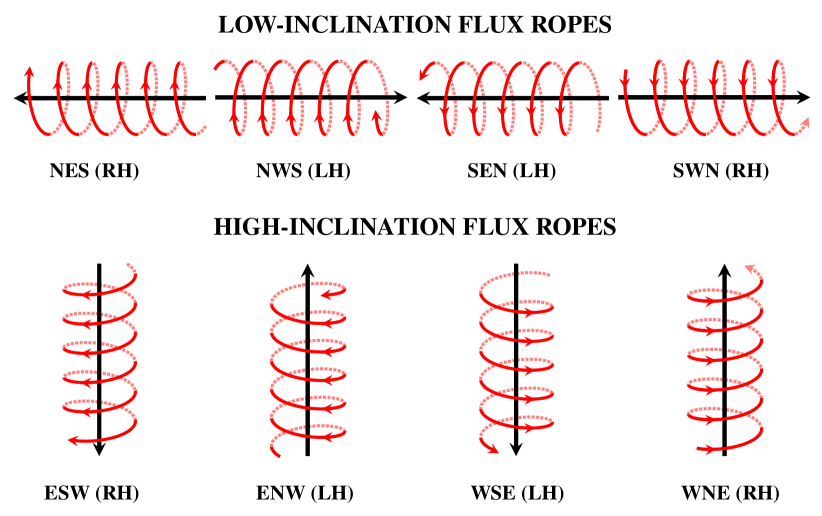
Figure 1: Sketch representing the eight main flux rope types and how the helical (in red) and axial (in black) magnetic fields are related to each other for each type. Each letter describing a type represents one of the four directions (North, West, South, and East), while RH indicates right-handed and LH indicates left-handed helicity. This classification follows Bothmer and Schwenn (1998) and Mulligan et al. (1998).

At present, it is not possible to determine the magnetic structure of erupting flux ropes in the corona from direct observations of the magnetic field. However, several indirect proxies based on EUV, X-ray, and photospheric magnetograms have been used to estimate the “intrinsic” flux rope type at the time of eruption. In several studies, such proxies have been used to estimate the magnetic structure of erupting CMEs, which have been compared to in situ observations (e.g., McAllister et al., 2001; Yurchyshyn et al., 2001; Möstl et al., 2008; Palmerio et al., 2017). These studies have been based either on observations alone or on observations combined with theoretical and/or empirical models. In order to reconstruct the intrinsic flux rope type, the chirality sign, the axis tilt (i.e., its inclination to the ecliptic), and the axial direction of the magnetic field have to be known. In a force-free magnetic field configuration like a flux rope, the total magnetic helicity is conserved (Woltjer, 1958). Previous studies have suggested that the helicity sign, the total helicity, and the total magnetic flux of an ICME flux rope are related to those of its corresponding source region (e.g., Leamon et al., 2004; Qiu et al., 2007; Möstl et al., 2009; Cho et al., 2013; Hu et al., 2014; Pal et al., 2017). Hence, the property of magnetic helicity conservation can be used to assume that once the flux rope type at the Sun is determined, its chirality is maintained as the CME propagates from the Sun to Earth.

Palmerio et al. (2017) determined the magnetic structure of two CMEs both at the Sun and in situ. The scheme presented in their work is based on the combination of multiwavelength remote-sensing observations in order to determine the chirality of the erupting flux rope and the inclination and direction of its axial field, thus reconstructing the intrinsic flux rope type. While, for the two eruptions under study, the flux rope type was the same when determined at the Sun as when measured in situ at the Lagrange L1 point, this is not universally the case. CMEs can change their orientation due to deflections (e.g., Kay et al., 2013; Wang et al., 2014), rotations (e.g., Möstl et al., 2008; Vourlidas et al., 2013; Isavnin et al., 2014), and deformations (e.g., Savani et al., 2010) in the corona and in interplanetary space, and this can alter the classification of the flux rope. CMEs can also change their direction, orientation, and shape due to interaction with other CMEs or corotating interaction regions (CIRs, Lugaz et al., 2012; Shen et al., 2012). In addition, it is often difficult to predict how close a flux rope will cross Earth with respect to its nose and its central axis, and in some cases even whether a CME will encounter Earth at all (e.g., Möstl et al., 2014; Mays et al., 2015; Kay et al., 2017).

In this work, we extend the study of Palmerio et al. (2017). In particular, we quantify the success of predicting flux rope types when neglecting CME evolution through a statistical analysis. The methods described by Palmerio et al. (2017) provide a relatively quick and straightforward estimate of the flux rope type for space weather forecasting purposes. However, due to the potentially significant evolution of flux ropes in the corona and heliosphere through the previously described processes, the applicability of the approach has to be statistically evaluated. This is the key motivation for this study. We point out that irrespective of any direct correspondence that is found between intrinsic and in situ flux rope types, the Palmerio et al. (2017) scheme can provide a crucial input to semi-empirical CME models (e.g., Savani et al., 2015, 2017; Kay et al., 2016, 2017) or flux rope models used in numerical simulations (e.g., Shiota and Kataoka, 2016) that can capture the evolution. Apart from the CME evolution in the corona, changes in the axis orientation may be related to either global rotations of the whole CME body and/or to local deformations of the flux rope during its travel in the interplanetary medium, and/or to limitations of the methods used to determine the CME orientation both at the Sun and in situ.

This paper is organised as follows. In Section 2, we describe the spacecraft and ground-based data that we use, and also introduce the catalogue of events that we consider for this study. Then, we discuss in more detail the different methods that we have applied to determine the intrinsic flux rope type at the point of the eruption, from solar observations, and the in situ analysis we performed. In Section 3, we apply our methods to 20 Earth-directed CMEs, by estimating the intrinsic flux rope type and comparing it to the magnetic structure measured near Earth. Finally, in Section 4, we discuss and summarize our results.

2 Data and Methods

2.1 Spacecraft and Ground-based Data

We combine various remote-sensing observations to estimate the intrinsic flux rope type of the CMEs under study and to link the interplanetary structures to their solar origins.

We use coronagraph images taken with the Large Angle Spectroscopic Coronagraph (LASCO: Brueckner et al., 1995) onboard the Solar and Heliospheric Observatory (SOHO: Domingo et al., 1995) and with the COR1 and COR2 coronagraphs that form part of the Sun Earth Connection Coronal and Heliospheric Investigation (SECCHI: Howard et al., 2008) instrument package onboard the Solar Terrestrial Relations Observatory (STEREO: Kaiser et al., 2008). The Heliospheric Imagers (HI: Eyles et al., 2009) onboard STEREO are also used, primarily to connect the CMEs with their corresponding ICMEs.

We also use EUV/UV images and line-of-sight magnetograms taken with the Atmospheric Imaging Assembly (AIA: Lemen et al., 2012) and the Helioseismic and Magnetic Imager (HMI: Scherrer et al., 2012) instruments onboard the Solar Dynamics Observatory (SDO: Pesnell et al., 2012). AIA takes images with a pixel size of 0.6 arcsec and a cadence of 12 seconds. HMI creates full-disc magnetograms using the 6173 Å  spectral line with a pixel size of 0.5 arcsec and a cadence of 45 seconds. During gaps in the AIA dataset, we use observations from the Sun-Watcher with Active Pixel System and Image Processing (SWAP: Berghmans et al., 2006) instrument onboard the Project for On Board Autonomy 2 (PROBA2) that images the Sun at 174 Å  with a cadence of one minute.

Soft X-ray data are supplied by the X-Ray Telescope (XRT: Golub et al., 2007) onboard Hinode (Solar-B: Kosugi et al., 2007). XRT has various focal plane analysis filters, detecting X-ray emission over a wide temperature range (from 1 to 10 MK). It provides images with a pixel size of two-arcseconds.

We use H$\alpha$ (6563 Å) observations from the Global Oscillations Network Group (GONG) and the Global High Resolution H$\alpha$ Network (HANET). GONG is a six-station network and HANET is a seven-station network of ground-based observatories located around the Earth to provide near-continuous observations of the Sun.

In situ measurements are taken from the Wind satellite. In particular, we use the data from the Wind Magnetic Fields Investigation (MFI: Lepping et al., 1995) and the Wind Solar Wind Experiment (SWE: Ogilvie et al., 1995), which provide 60-second and 90-second resolution data, respectively.

Hourly disturbance storm time (Dst) values are taken from the WDC for Geomagnetism, Kyoto, webpage (http://wdc.kugi.kyoto-u.ac.jp/wdc/Sec3.html). The events until 2013 are based on the final Dst index, while those from 2014 and 2015 are based on the provisional Dst index.

2.2 Event Selection

We searched the LINKed CATalogue (LINKCAT) for suitable events. LINKCAT is an output of the HELiospheric Cataloguing, Analysis and Techniques Service (HELCATS, https://www.helcats-fp7.eu) project and contains events in the timerange May 2007 to December 2013. LINKCAT connects CMEs from their solar source to their in situ counterparts using a geometrical fitting technique based on single spacecraft data from the STEREO/HI instruments. CME tracks in HI time-elongation maps (so-called J-maps) are fitted using the Self-Similar Expansion Fitting (SSEF) method (Davies et al., 2012), assuming a fixed angular half-width of $30^{\circ}$ for each CME. This yields estimates of a CME’s propagation direction and radial speed. The LINKCAT catalogue consists of events where CMEs observed in HI imagery could be uniquely linked to CMEs observed in coronagraph and solar disc data and ICMEs detected in situ.This was done by ensuring that the predicted impact of the CME based on SSEF is within $\pm 24$ hrs of the in situ arrival time (often this is the shock arrival time). Cases where two CMEs are predicted to arrive within this window, or two ICMEs are detected within the window, are excluded, eliminating potential CME–CME interaction events. More details can be found in the online information pertaining to the catalogue (see Sources of Data and Supplementary Material). It must be kept in mind when thinking about real-time prediction that our study thus involves the down-selection to cases of a particular nature, and is based on science data. One of the ICME catalogues used to compile LINKCAT, in particular for CMEs detected towards Earth, is the Wind ICME catalogue (https://wind.nasa.gov/ICMEindex.php). For a validation of use of the aforementioned HI-based SSEF technique to predict CME arrivals, see Möstl et al. (2017).

Since SDO is our primary spacecraft for solar observations to study the CME source region, only the LINKCAT events that arrived at Earth after May 2010 are considered. During this period, LINKCAT contains 47 Earth-impacting events. We further consider only events that present a clear flux rope in situ, i.e. from which we are able to estimate the flux rope type by visual inspection. We are left with 12 CME–ICME pairs. Since LINKCAT is compiled in a semi-automated way, we also performed our own survey of on-disc CME signatures in SDO images for the events in the LINKCAT catalogue. Due to some restrictive assumptions (e.g. $30^{\circ}$ fixed angular half width), LINKCAT does not include all possible CME–ICME pairs.

Therefore, to find additional events for analysis we also searched other ICME catalogues, identifying ICMEs for which we could find the corresponding solar source over the period corresponding to SDO observations. In particular, we searched for additional in situ flux ropes from the Wind ICME list and from the Near-Earth Interplanetary Coronal Mass Ejections list (http://www.srl.caltech.edu/ACE/ASC/DATA/level3/icmetable2.htm). We scanned backwards from the time at which events were observed by the HI imagers, identifying corresponding signatures in images from the COR2 and COR1 coronagraphs, and finally searched for the source on the solar disc. For those events that were not in LINKCAT, we tracked the ICME backwards in time to the Sun assuming constant speed and radial propagation, and used HI imagery to follow the CME in the heliosphere. At this stage, we utilised the HELCATS ARRival CATalogue (ARRCAT, Möstl et al., 2017), that lists predicted arrivals of CMEs at various spacecraft and planets using the previously described STEREO/HI SSEF fitting technique.

In the search for additional events, we also extended the time range of the data under consideration to December 2015. We identify eight additional events in this way (two due to the extension of the time range), bringing the total number of events in the study up to 20. We number the events (1–20) in chronological order of their launch times; the additional events correspond to those numbered 2, 3, 9, 10, 11, 15, 19, and 20. Event number 10 is a CME–CME interaction event in June 2012 for which the CME–ICME relation has been clarified in several previous studies (e.g., Kubicka et al., 2016; Palmerio et al., 2017; James et al., 2017; Srivastava et al., 2018). Event number 18 is a lineup event which was also partly observed by MESSENGER, situated only a few degrees away from the Sun–Earth line (Möstl et al., 2018).

2.3 Intrinsic Flux Rope Type Determination

As mentioned in the Introduction, in order to determine the magnetic flux rope type of an erupting CME, three parameters are needed: the chirality, the axis orientation, and the axial field direction. The chirality can be inferred from several multi-wavelength proxies: magnetic tongues (López Fuentes et al., 2000; Luoni et al., 2011), X-ray and/or EUV sigmoids and/or sheared arcades (e.g., Rust and Kumar, 1996; Canfield et al., 1999; Green et al., 2007), the skew of coronal arcades (McAllister et al., 1998; Martin et al., 2012), flare ribbons (Démoulin et al., 1996), and filament details (Martin et al., 1994; Martin and McAllister, 1996; Chae, 2000). For a detailed description of these helicity proxies, see Palmerio et al. (2017).

The inclination of the flux rope axis with respect to the ecliptic, $\tau$, is taken to be the average of the orientation of the polarity inversion line (PIL, Marubashi et al., 2015) and the orientation of the post-eruption arcades (PEAs, Yurchyshyn, 2008), in the range $[-90^{\circ},90^{\circ}]$. The tilt angle $\tau$ is measured from the solar East, and assumes a positive (negative) value if the acute angle to the ecliptic is to the North (South). For source regions where the PIL can easily be approximated as a straight line (e.g., quiet Sun and magnetically simple active regions), we determine the PIL orientation by eye, i.e. we determine the location where the polarity of the magnetic field reverses, and approximate it as a straight line. When the PIL is more curved and/or complex, we smooth the data over square bins containing variable numbers of pixels, overplot the locations where $B_{r}=0$, and then estimate the orientation of the resulting PIL. For source regions located between $\pm 30^{\circ}$ in longitude on the solar disc, we use HMI line-of-sight data. For source regions located closer to the limb, in order to reduce the projection effects, we use Space-weather HMI Active Region Patch (SHARP: Bobra et al., 2014) data, derived with the series hmi.sharp_cea_720s where the vector B has been remapped onto a Lambert Cylindrical Equal-Area (CEA) projection. Similarly, the orientation of the PEAs is determined by eye for source regions located between $\pm 30^{\circ}$ in longitude on the solar disc, while for regions located nearer the limb, we correct the projection effects by first converting two points on the arcade axis from Helioprojective-Cartesian to Heliographic coordinates. Then, we apply to the axis the vector rotation operator “rotate”, defined as

$$\text{rotate}(\mathbf{\hat{v}},\mathbf{\hat{a}},\gamma)=\mathbf{\hat{v}}\cos{\gamma}+(\mathbf{\hat{v}}\cdot\mathbf{\hat{a}})(1-\cos{\gamma})\mathbf{\hat{a}}+[\mathbf{\hat{a}}\times\mathbf{\hat{v}}]\sin{\gamma}\,,$$ (1)

which rotates the arcade axis, $\mathbf{\hat{v}}$, counterclockwise around its median, $\mathbf{\hat{a}}$, by a tilt angle, $\gamma$ (Isavnin et al., 2013). We rotate the axis until it becomes parallel to the ecliptic. The total rotation corresponds to the unprojected tilt of the arcade’s axis.

For some events, we could only estimate the orientation of the axis from the PIL direction, because PEAs were either too short or not visible. When we have obtained the average orientation between PIL and PEAs, we assume:

1. $0^{\circ}\leq|\tau|<35^{\circ}\Rightarrow$ low-inclination flux rope

2. $35^{\circ}\leq|\tau|\leq 55^{\circ}\Rightarrow$ intermediate flux rope

3. $55^{\circ}<|\tau|\leq 90^{\circ}\Rightarrow$ high-inclination flux rope

Finally, we check the direction of the axial field by looking at coronal dimmings in EUV difference images and identifying in which magnetic polarities they are rooted. Then, the magnetic field direction is defined from the positive polarity to the negative one. When the three parameters are known, we can reconstruct the flux rope type at the point of the eruption.

2.4 In situ Flux Rope Type Identification

The CME flux rope type at the time of the eruption is compared to the magnetic configuration of the corresponding ICME. First, we analyse, by eye, the magnetic field components of the ICME observed in situ in both Cartesian ($B_{x}$, $B_{y}$, $B_{z}$) and angular ($B_{\theta}$, $B_{\phi}$) geocentric solar ecliptic (GSE) coordinates, and make a first estimate of the type of the in situ flux rope.

We then apply minimum variance analysis (MVA, Sonnerup and Cahill, 1967) to the in situ measurements during the flux rope interval, to estimate the orientation of the flux rope axis (latitude, $\theta_{\text{MVA}}$, and longitude, $\phi_{\text{MVA}}$) and obtain its helicity sign. The latter is done by inspection of the direction of the magnetic field rotation in the intermediate-to-maximum plane. The flux rope axis corresponds to the MVA intermediate variance direction, where $\theta_{\text{MVA}}=90^{\circ}$ is defined as being northward and $\phi_{\text{MVA}}=90^{\circ}$ is defined as being eastward. We apply the MVA to 20-minute averaged magnetic field data. We also consider the intermediate-to-mininum eigenvalue ratio ($\lambda_{2}/\lambda_{3}$) resulting from MVA. MVA can be considered most reliable when $\lambda_{2}/\lambda_{3}\geq 2$ (e.g., Lepping and Behannon, 1980; Bothmer and Schwenn, 1998; Huttunen et al., 2005).

As a proxy for the spacecraft crossing distance from the flux rope central axis (or impact parameter), we calculate the ratio of the minimum variance direction to the total magnetic field in the MVA frame (Gulisano et al., 2007; Démoulin and Dasso, 2009), $\langle|B_{\min}|\rangle/\langle B\rangle$. We average the quantities along the whole flux rope interval. A higher ratio indicates that the flux rope has been crossed progressively farther from its central axis, and it implies that the bias in the flux rope orientation is larger.

As a proxy for the spacecraft crossing distance from the nose of the flux rope, we calculate the location angle, L, defined by Janvier et al. (2013) as

$$\text{sin}\,\text{L}=\text{cos}\,\theta_{\text{MVA}}\,\text{cos}\,\phi_{\text{MVA}}\,.$$ (2)

The location angle ranges from $\text{L}\approx-90^{\circ}$ in one leg, through $\text{L}\approx 0^{\circ}$ at the nose, to $\text{L}\approx 90^{\circ}$ in the other leg.

Finally, we check the minimum value of the (Dst) index related to each event. We only quote the events for which Dst${}_{\text{min}}<-50$. We consider those events with $-50$ ¿ Dst${}_{\text{min}}>-100$ as moderate storms, and those events for which Dst${}_{\text{min}}\leq-100$ as major storms.

2.5 Orientation Angles

The next step is to compare the orientations of the CME axis at the Sun and in situ. Regarding the former, we convert the tilt angle, $\tau$, into the orientation angle, $\alpha_{\text{SUN}}$, that lies within the range $[-180^{\circ},180^{\circ}]$. $\alpha_{\text{SUN}}$ is derived from $\tau$ by taking into account in which direction the flux rope axial field is pointing, that was previously estimated from coronal dimmings (see Section 2.3). The orientation angle is calculated from the positive East direction, clockwise for positive values and counterclockwise for negative values. Yurchyshyn (2008) determined the flux rope orientation of 25 CME events at the Sun from PEAs only, and estimated that the PEAs angles were measured with accuracy $\pm 10^{\circ}$ for 19 events, and $\pm 90^{\circ}$ for the remaining six. Since our flux rope orientations at the Sun are determined by a combination of PIL and PEAs, we estimate that the tilt angles were measured with an accuracy between $\pm 5^{\circ}$ (for the cases where PIL and PEAs had an almost identical orientation) and $\pm 15^{\circ}$–$20^{\circ}$ (for the cases when we could only use the PIL direction, or the PIL and PEAs directions had a larger angular separation).

Regarding the orientation of the in situ flux rope at the Lagrange L1 point, we project the axis resulting from the MVA analysis onto a 2D plane that corresponds to the YZ-plane in GSE coordinates. We then measure the in situ clock angle orientation, $\alpha_{\text{L1}}$, within the range $[-180^{\circ},180^{\circ}]$ as for $\alpha_{\text{SUN}}$. The MVA fittings introduce an error of $\pm 5^{\circ}$–$10^{\circ}$ when the spacecraft crosses the flux rope axis approximately perpendicularly. However, for crossings that are progressively farther from the central axis, the error on the estimated flux rope axis orientation can be up to $\pm 90^{\circ}$ (Owens et al., 2012). In particular, Gulisano et al. (2007) studied in detail the bias introduced in MVA fittings for flux ropes. They found that $\theta_{\text{MVA}}$ is best determined for flux ropes that have their axis close to the ecliptic plane and nearly perpendicular to the Sun-Earth line. Moreover, the angle $\eta$ between the true flux rope orientation and the MVA-generated one is $\eta\approx 3^{\circ}$ for a spacecraft crossing a cloud within 30% of its radius, and $\eta\lesssim 20^{\circ}$ for an impact parameter as high as 90% of the flux rope radius. One of the main issues in flux rope fittings with MVA is, therefore, the fact that the impact parameter is unknown.

3 Results

The source regions of the 20 analysed CMEs have the following properties:

• 10 (50%) CMEs erupted from the Northern hemisphere and 10 (50%) from the Southern hemisphere.

• 14 (70%) CMEs erupted from an active region, two (10%) from between two active regions, and four (20%) from a quiet Sun filament.

• 18 (90%) of source regions followed the hemispheric helicity rule, while two (10%) did not.

Table 1 shows which helicity sign proxies were used for each event. The proxy that we could use the most (applicable to 18 events or 90%) is the skew of the coronal arcades. This is not surprising, considering that most CMEs are associated with arcades before and/or after an eruption. These arcades can either be the coronal loops that overlie the eruptive structure or arcades that form under the CME due to magnetic reconnection after it is ejected. In a few cases, however, the arcade skew was not clear enough to be used as a helicity proxy. Clear S-shaped features were found for 14 (70%) events. We consider here both sheared arcades and sigmoids, which are structures that can be seen in X-ray and sometimes also in EUV. Sheared arcades are multi-loop systems, while sigmoids are single-loop S-shaped structures (e.g., Green et al., 2007). Sigmoids and arcades that have forward (reverse) S-shape indicate positive (negative) helicity. Another popular chirality proxy is the use of flare ribbons. We were able to use this proxy for 11 (55%) events. It is worth remarking that flare ribbons can be used to estimate the helicity sign of a CME and its source region if they form clear J-shapes, where a forward (reverse) J indicates positive (negative) helicity, or if they are significantly shifted along the PIL. A filament association was found for 12 (60%) CMEs, and for all of these we were able to use filament characteristics to estimate the chirality. We analysed both H$\alpha$ details, i.e. filament spine shape and barbs, and EUV details, i.e. the crossings of dark and bright threads. H$\alpha$ characteristics are mostly visible in quiet Sun filaments, while absorption and emission threads are mostly visible in active region filaments. Only for one event (Event 9) were we able to analyse the filament successfully both in H$\alpha$ and EUV. The least applicable proxy involves the use of magnetic tongues. We were only able to apply this technique to three (15%) events. This is expected, as magnetic tongues are only visible in emerging active regions. Finally, we emphasize that, for each analysed event, all helicity sign proxies agree with one another.

Table 1: A summary of the chirality and shear determinations used for each of the CMEs studied. The table shows, from left to right: event number, Solar Object Locator (SOL), eruption time rounded to the nearest hour, and the chirality made possible due to the presence of magnetic tongues, proxies visible in H$\alpha$ related to the chirality of a filament, absorption and emission filament threads visible in EUV, S-shaped structure (sheared arcade or sigmoid) in EUV or X-rays, skew of coronal loops, and J-shaped flare ribbons.

#	Eruption	Tongues	H$\alpha$-fil	EUV-fil	S-shape	Skew	Ribbons
1	SOL2010-05-23, 17 UT	-	LH	-	-	LH	-
2	SOL2011-03-25, 06 UT	-	-	-	-	RH	-
3	SOL2011-06-02, 07 UT	-	-	RH	RH	RH	-
4	SOL2011-09-13, 22 UT	-	-	-	LH	LH	-
5	SOL2011-10-22, 01 UT	-	LH	-	-	LH	LH
6	SOL2012-01-19, 14 UT	-	-	-	-	LH	LH
7	SOL2012-03-10, 17 UT	LH	-	LH	LH	LH	LH
8	SOL2012-03-13, 17 UT	LH	-	LH	LH	LH	LH
9	SOL2012-05-11, 23 UT	-	RH	RH	RH	RH	RH
10	SOL2012-06-14, 13 UT	RH	-	-	RH	RH	-
11	SOL2012-07-04, 17 UT	-	-	LH	LH	LH	LH
12	SOL2012-07-12, 16 UT	-	-	RH	RH	RH	RH
13	SOL2012-10-05, 00 UT	-	-	-	RH	-	-
14	SOL2012-10-08, 21 UT	-	-	-	LH	LH	-
15	SOL2012-10-27, 12 UT	-	-	-	-	RH	-
16	SOL2013-01-13, 00 UT	-	-	-	RH	RH	-
17	SOL2013-04-11, 07 UT	-	-	LH	LH	-	LH
18	SOL2013-07-09, 14 UT	-	LH	-	LH	LH	LH
19	SOL2014-08-15, 16 UT	-	RH	-	-	RH	RH
20	SOL2015-12-16, 08 UT	-	-	RH	RH	RH	RH

Table 2 lists the estimated flux rope types at the Sun and Table 3 the local flux rope types observed in situ. We note that the chirality of the intrinsic flux rope and in situ flux rope matched for all 20 events, including the two events that did not follow the hemispheric helicity rule. This result is expected, as the helicity sign should be preserved during interplanetary propagation, and it also gives further confirmation that our indirect helicity proxies derived from solar observations are correct. For two events (numbers 6 and 16), the MVA intermediate-to-medium eigenvalue ratio was $\lambda_{2}/\lambda_{3}<2$, but the flux rope orientation resulting from MVA agreed with the flux rope type obtained from visual inspection.

Table 2: The results of the analysis of the magnetic structure of the flux rope on the Sun. The table shows, from left to right: event number, Solar Object Locator (SOL), eruption time rounded to the nearest hour, CME source (QS: Quiet Sun, NH: Northern Hemisphere, SH: Southern Hemisphere, AR: Active Region), chirality of the erupting flux rope, whether the chirality follows the hemispheric helicity rule (HHR), inclination of the PIL, inclination of the PEAs, average tilt of the axis with respect to the ecliptic plane, direction of the axial field, and erupting flux rope type.

#	CME
	SOL	Eruption time	Source	Chirality	HHR	PIL	PEAs	Tilt	Axial field	FR type
1	SOL2010-05-23	17 UT	QS, NH	LH	Yes	$38^{\circ}$	$50^{\circ}$	$44^{\circ}$	Southwest	WSE/NWS
2	SOL2011-03-25	06 UT	AR 11176	RH	Yes	$-86^{\circ}$	–	$-86^{\circ}$	South	ESW
3	SOL2011-06-02	07 UT	AR 11226/11227	RH	Yes	$-45^{\circ}$	–	$-45^{\circ}$	Northwest	WNE/SWN
4	SOL2011-09-13	22 UT	AR 11289	LH	Yes	$40^{\circ}$	$40^{\circ}$	$40^{\circ}$	Southwest	WSE/NWS
5	SOL2011-10-22	01 UT	QS, NH	LH	Yes	$32^{\circ}$	$34^{\circ}$	$33^{\circ}$	East	SEN
6	SOL2012-01-19	14 UT	AR 11402	LH	Yes	$-80^{\circ}$	$-88^{\circ}$	$-84^{\circ}$	South	WSE
7	SOL2012-03-10	17 UT	AR 11429	LH	Yes	$26^{\circ}$	$38^{\circ}$	$32^{\circ}$	East	SEN
8	SOL2012-03-13	17 UT	AR 11429	LH	Yes	$40^{\circ}$	$46^{\circ}$	$43^{\circ}$	Northeast	ENW/SEN
9	SOL2012-05-11	23 UT	small AR, SH	RH	Yes	$-65^{\circ}$	$-65^{\circ}$	$-65^{\circ}$	South	ESW
10	SOL2012-06-14	13 UT	AR 11504	RH	Yes	$-30^{\circ}$	–	$-30^{\circ}$	East	NES
11	SOL2012-07-04	17 UT	AR 11513	LH	Yes	$46^{\circ}$	$36^{\circ}$	$41^{\circ}$	Southwest	WSE/NWS
12	SOL2012-07-12	16 UT	AR 11520	RH	Yes	$-30^{\circ}$	$-14^{\circ}$	$-22^{\circ}$	East	NES
13	SOL2012-10-05	00 UT	AR 11582/11584	RH	Yes	$-73^{\circ}$	–	$-73^{\circ}$	South	ESW
14	SOL2012-10-08	21 UT	AR 11585	LH	No	$47^{\circ}$	–	$47^{\circ}$	Northeast	ENW/SEN
15	SOL2012-10-27	12 UT	AR 11598	RH	Yes	$-50^{\circ}$	–	$-50^{\circ}$	Southeast	ESW/NES
16	SOL2013-01-13	00 UT	AR 11654	RH	No	$-88^{\circ}$	–	$-88^{\circ}$	North	WNE
17	SOL2013-04-11	07 UT	AR 11719	LH	Yes	$60^{\circ}$	$50^{\circ}$	$55^{\circ}$	Southwest	WSE/NWS
18	SOL2013-07-09	14 UT	QS, NH	LH	Yes	$47^{\circ}$	$53^{\circ}$	$50^{\circ}$	Southwest	WSE/NWS
19	SOL2014-08-15	16 UT	QS, SH	RH	Yes	$82^{\circ}$	$70^{\circ}$	$76^{\circ}$	North	WNE
20	SOL2015-12-16	08 UT	AR 12468	RH	Yes	$-32^{\circ}$	$-24^{\circ}$	$-28^{\circ}$	East	NES

Table 3: The results of the analysis of the magnetic structure of the flux rope in situ. The table shows, from left to right: arrival time of the ICME flux rope leading edge, time of the ICME flux rope trailing edge, chirality of the in situ flux rope, flux rope axis from MVA in the form (latitude, longitude), MVA intermediate-to-minimum eigenvalue ratio, ratio of the MVA minimum variance component to the total magnetic field (proxy for the impact parameter or crossing distance from the ICME axis), location angle (proxy for the crossing distance from the ICME nose), minimum Dst index value (only for events Dst ¡ -50), and in situ flux rope type from visual inspection.

#	ICME
	Leading Edge	Trailing Edge	Chirality	MVA Axis	$\lambda_{2}/\lambda_{3}$	$\langle|B_{\min}|\rangle/\langle B\rangle$	L-angle	Dst${}_{\text{min}}$	FR type
1	2010-05-28, 19:10	2010-05-29, 16:50	LH	($-59^{\circ}$, $234^{\circ}$)	17.9	0.08	$-18^{\circ}$	$-80$	WSE
2	2011-03-30, 00:25	2011-04-01, 15:05	RH	($17^{\circ}$, $119^{\circ}$)	2.9	0.13	$-28^{\circ}$	–	NES
3	2011-06-05, 01:58	2011-06-05, 08:55	RH	($68^{\circ}$, $135^{\circ}$)	3.9	0.10	$-15^{\circ}$	–	WNE
4	2011-09-17, 15:38	2011-09-18, 08:46	LH	($46^{\circ}$, $70^{\circ}$)	4.5	0.19	$14^{\circ}$	$-72$	ENW/SEN
5	2011-10-25, 00:30	2011-10-25, 17:09	LH	($74^{\circ}$, $56^{\circ}$)	2.7	0.22	$9^{\circ}$	$-147$	ENW
6	2012-01-22, 11:40	2012-01-23, 07:55	LH	($-49^{\circ}$, $263^{\circ}$)	1.9	0.48	$-5^{\circ}$	$-71$	NWS/WSE
7	2012-03-12, 10:05	2012-03-12, 14:55	LH	($-16^{\circ}$, $35^{\circ}$)	2.6	0.45	$52^{\circ}$	$-64$	SEN
8	2012-03-15, 15:52	2012-03-16, 14:06	LH	($65^{\circ}$, $105^{\circ}$)	2.2	0.39	$-6^{\circ}$	$-88$	ENW
9	2012-05-16, 16:00	2012-05-17, 22:20	RH	($46^{\circ}$, $271^{\circ}$)	27.9	0.17	$1^{\circ}$	–	SWN/WNE
10	2012-06-16, 22:10	2012-06-17, 12:30	RH	($-28^{\circ}$, $99^{\circ}$)	19.3	0.10	$-8^{\circ}$	$-86$	NES
11	2012-07-08, 23:48	2012-07-09, 20:56	LH	($-50^{\circ}$, $340^{\circ}$)	5.2	0.38	$37^{\circ}$	$-78$	WSE
12	2012-07-15, 06:16	2012-07-16, 14:33	RH	($-4^{\circ}$, $305^{\circ}$)	5.8	0.57	$35^{\circ}$	$-139$	ESW
13	2012-10-08, 17:15	2012-10-09, 13:34	RH	($-66^{\circ}$, $258^{\circ}$)	8.9	0.30	$-5^{\circ}$	$-109$	ESW
14	2012-10-12, 15:50	2012-10-13, 09:42	LH	($-60^{\circ}$, $247^{\circ}$)	10.6	0.38	$-11^{\circ}$	$-90$	WSE
15	2012-10-31, 23:32	2012-11-02, 02:30	RH	($-68^{\circ}$, $49^{\circ}$)	51.2	0.12	$14^{\circ}$	$-65$	ESW
16	2013-01-17, 16:13	2013-01-18, 11:48	RH	($18^{\circ}$, $250^{\circ}$)	1.4	0.16	$-19^{\circ}$	$-52$	SWN
17	2013-04-14, 16:10	2013-04-15, 20:42	LH	($62^{\circ}$, $337^{\circ}$)	6.4	0.17	$26^{\circ}$	–	ENW
18	2013-07-13, 04:55	2013-07-14, 23:30	LH	($-10^{\circ}$, $286^{\circ}$)	13.5	0.08	$16^{\circ}$	$-81$	NWS
19	2014-08-19, 17:25	2014-08-21, 00:07	RH	($65^{\circ}$, $314^{\circ}$)	48.5	0.07	$17^{\circ}$	–	WNE
20	2015-12-20, 02:55	2015-12-21, 20:25	RH	($-30^{\circ}$, $221^{\circ}$)	3.8	0.43	$-41^{\circ}$	$-155$	ESW

The flux rope types (Figure 1) at the Sun and in situ match strictly for only four (20%) of the 20 events (Events 7, 10, 13, and 19). Figure 2 gives an example of such an event (Event 10). Figure 2a shows an SDO/HMI line-of-sight (LOS) magnetogram approximately two days before the eruption, when the active region was emerging, revealing the presence of right-handed magnetic tongues. Figure 2b shows a sigmoid seen in EUV that also suggests positive helicity. Another helicity proxy that we used for this event is the skew of arcade loops (not shown). The orientation of the neutral line is shown in panel 2c and has a tilt $\tau=-30^{\circ}$. The axial field points to the East. As explained in Section 2.3, this can be deduced from the locations of the EUV dimmings associated with the flux rope footpoints that are overlaid with SDO/HMI magnetogram data (Figure 2d). The previously described solar observations yield a NES-type flux rope. In situ observations are shown on the right-hand side of Figure 2. The ICME was preceded by a shock (red line), and the flux rope (bounded between the pair of blue lines) is clearly identified from the enhanced magnetic field and smooth rotation of the field direction. MVA yields the axis of tilt $-28^{\circ}$, the fact that the field at the axis points to the East, and that the chirality is right-handed. Hence, the flux rope type in situ is also NES, and the axis tilts at the Sun and in situ are almost identical.

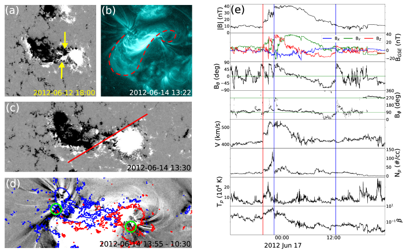
Figure 2: Event 10, which is found to be a NES-type both at the Sun and in situ. (a) Magnetic tongues as seen in an SDO/HMI magnetogram (saturated at $\pm 200$ G) that show positive chirality. (b) Forward-S sigmoid as seen by SDO/AIA 131 Å  that indicates a right-handed flux rope. (c) HMI magnetogram (saturated at $\pm 200$ G) showing the PIL approximated as a straight line (in red). (d) Base-difference AIA image in 131 Å  saturated at $\pm 70$ DN s^-1 pixel^-1 and overlaid with HMI magnetogram contours saturated at $\pm 200$ G (blue = negative polarity, red = positive polarity). The dimming regions (signatures of the flux rope footpoints) have been circled in green. (e) The ICME as observed in situ by Wind. The red line indicates the arrival of the IP shock, while the blue lines indicate the leading and trailing edges of the flux rope. The parameters shown are, from top to bottom: magnetic field magnitude, magnetic field components in GSE cartesian coordinates, $\theta$ and $\phi$ components of the magnetic field in GSE angular coordinates, solar wind speed, proton density, proton temperature, and plasma $\beta$.

We emphasize that, for a significant fraction of events (nine or 45%), the tilt angle at the Sun and/or the latitude of the in situ flux rope axis was close to $45^{\circ}$. For such cases, considering the possible errors, one cannot distinguish between low and high-inclination flux rope types. We categorise these cases as intermediate-inclination events (see Section 2.3). An example of such an event is Event 18 (Figure 3). The left-handed chirality of this event could be determined at the Sun from H$\alpha$ filament details, arcade skew, flare ribbons, and S-shape of the filament seen in EUV. The average between the PIL tilt (Figure 3c) and the PEAs’ tilt (not shown) gives a tilt angle at the Sun of $50^{\circ}$. The axial field points to the Southwest, i.e. the possible intrinsic flux rope types are either a high-inclination WSE flux rope or a low-inclination NWS flux rope. The in situ data, again, show a clear flux rope identified from enhanced magnetic field magnitude and smooth field rotation. The MVA yields an axis tilt of $10^{\circ}$ and left-handed chirality. Hence, the in situ flux rope clearly has a low-inclination and is of type NWS. If we also consider as a match cases where the flux rope is of intermediate type (i.e. close to $45^{\circ}$ inclination at the Sun and/or in situ), then the flux rope types agree between the Sun and in situ for 11 (55%) analysed events.

Figure 3: Event 18, which is intermediate between a WSE- and a NWS-type at the Sun and is a NWS-type in situ. (a) The reverse-S filament shape seen by SDO/AIA 171 Å  that indicates left-handed chirality. (b) Reverse-J shaped flare ribbons as seen in 304 Å, a sign of a left-handed flux rope. (c) SDO/HMI magnetogram (saturated at $\pm 200$ G) showing the PIL approximated as a straight line (in red). (d) Base-difference AIA image in 211 Å  saturated at $\pm 200$ DN s^-1 pixel^-1 and overlaid with HMI magnetogram contours saturated at $\pm 200$ G (blue = negative polarity, red = positive polarity). The dimming regions (signatures of the flux rope footpoints) have been circled in green. (e) The ICME as observed in situ by Wind (see Figure 2 for details).

A clear example of a case where the flux rope types at the Sun and in situ do not match is Event 17 (Figure 4). According to our analysis of the near-Sun observations, the intrinsic flux rope type is in the intermediate state between a high-inclination WSE-type and a low-inclination NWS-type. The helicity proxies that we used for this event were a clear reverse-S sigmoid (Figure 4a), a left-handed crossing of filament threads (Figure 4b), and reverse-J flare ribbons (visible in Figure 4d). The tilt angle at the Sun was estimated to be $55^{\circ}$. In this case, the tilt angle was deduced both from the PEAs seen in EUV (Figure 4c) and the orientation of the PIL (not shown). Visual inspection of the in situ measurements, however, shows a strongly northward field during the passage of the entire ICME, and suggests that the flux rope type is ENW. MVA yields a high-inclination flux rope with a tilt of $-62^{\circ}$, in agreement with the visual analysis. This means that the axis orientation changed by $\sim 180^{\circ}$ from the Sun to L1.

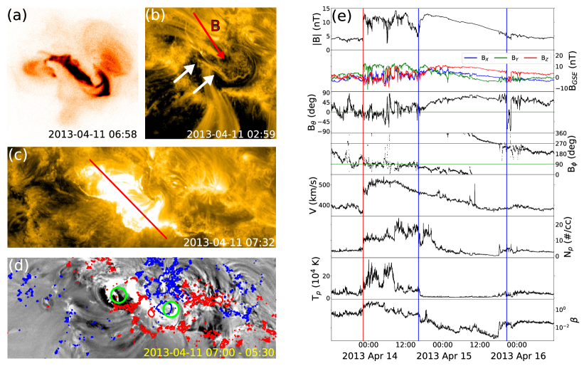
Figure 4: Event 17, which is intermediate between a WSE- and a NWS-type at the Sun and is an ENW-type in situ. (a) Reverse-colour soft X-ray images taken with Hinode/XRT, showing an erupting reverse-S sigmoid, indicative of a left-handed flux rope. Filter wheel 1 is in the “Beryllium thin” (Be thin) position, while filter wheel 2 is Open. (b) Left-handed crossings of filament threads (indicated by the white arrows) as seen by SDO/AIA in 171 Å. The direction of the magnetic field along the filament is also shown (in red). (c) 171 Å  observations showing the PEAs approximated as a straight line (in red). (d) Base-difference AIA image in 211 Å  saturated at $\pm 400$ DN s^-1 pixel^-1 and overlaid with HMI magnetogram contours saturated at $\pm 200$ G (blue = negative polarity, red = positive polarity). The dimming regions inside the reverse-J shapes of the flare ribbons (signatures of the flux rope footpoints) have been circled in green. (e) The ICME as observed in situ by Wind (see Figure 2 for details).

We also note that for two events (Events 12 and 20) the axis orientation resulting from MVA did not agree with our visual determination. Event 12 is clearly a case where the flux rope crosses Wind far from its centre; MVA does not perform well for such events. However for Event 20, it is not obvious why MVA yields a low-inclination flux rope ($\theta_{\text{MVA}}=30^{\circ}$), while observations suggests an intermediate event. Anyhow, the flux ropes types would not match between the Sun and L1, as the possible flux rope types in situ would be SWN and ESW.

The minimum Dst value for each analysed CME is reported in Table 3. We note that five (25%) CMEs caused minor or no storm (i.e., Dst${}_{\text{min}}$ ¿ -50 nT), 11 (55%) caused a moderate storm (-50 nT ¿ Dst${}_{\text{min}}$ ¿ -100 nT), and four (20%) caused an intense storm (Dst${}_{\text{min}}$ ¡ -100 nT). The six high-inclination flux ropes detected in situ with a southward axial field (i.e., of types ESW and WSE) all produced at least a moderate storm, and three of them produced intense storms. This is expected, since the primary requirement for a geomagnetic storm is that the interplanetary magnetic field is southward for a sufficiently long period of time. In total, our data set included five high-inclination and two “intermediate” ICMEs with northward axial fields. Four of these corresponded to minor or no storm (i.e., Dst${}_{\text{min}}$ ¿ -50 nT), but two (Events 4 and 8) caused moderate storms and one (Event 5), an intense storm. In these three events, Dst${}_{\text{min}}$ was reached either before or shortly after (within four hours of) the passage of the ICME leading edge over L1. This suggests that these storms were driven by the sheath ahead of the ICME. A significant fraction of magnetic storms are, in fact, purely sheath-driven (Tsurutani et al., 1988; Huttunen et al., 2002; Huttunen and Koskinen, 2004; Siscoe et al., 2007; Kilpua et al., 2017b). The sheaths of these three events, indeed, featured periods of strong southward fields (i.e., $B_{Z}\leq-10$ nT).

Figure 5 provides a visual representation of the results reported in Tables 2 and 3, by comparing the flux rope clock angles at the Sun to those at L1. The figure highlights how the expected flux rope type at Earth can change due to rotation of the flux rope axis in the corona or in interplanetary space. The events are grouped according to their chirality, in order to look for possible patterns that might be related to the sign of the helicity (i.e., clockwise rotation is expected for right-handed chirality and counterclockwise rotation for left-handed chirality, Fan and Gibson, 2003; Green et al., 2007; Lynch et al., 2009). We note from Figure 5 an obvious pattern: the axis clock angles at the Sun are clustered in the vicinity of the dashed lines both for left- and right-handed flux ropes (i.e., they lie along the Northwest–Southeast diagonal for right-handed events and the Northeast–Southwest diagonal for left-handed events). A similar pattern was found by Marubashi et al. (2015). The clock angle change from the Sun to Earth is ¡ $90^{\circ}$ for 13 (65%) events.

The remaining seven (35%) events experienced ¿ $90^{\circ}$ rotation of their central axis. Of these, one event (Event 2) experienced an apparent rotation of its axis by $\sim 100^{\circ}$, while the other six (30%) seemed to rotate by $\gtrsim 120^{\circ}$. Of these latter six cases, three events are right-handed and three events are left-handed. All of them were formed in active regions. Such large rotations have been reported previously in the literature (e.g., Harra et al., 2007; Kilpua et al., 2009). We have not considered here how the flux rope chirality affects the sense of rotation of the clock angle, because, in some cases, the MVA can have large errors related to the in situ clock angle (up to about $\pm 90^{\circ}$ when the flux rope is crossed very far from its central axis) and because, from a forecasting perspective, it is more useful to consider the smallest rotation angle between the two orientations (i.e., ¡ $\pm 180^{\circ}$).

We remark that a large fraction of events had their solar tilt angle close to $45^{\circ}$. In this regard, we point out that, when the flux rope axis orientation determined from solar observations is close to the intermediate one, the expected flux rope type at Earth can change even due to a relatively small amount of rotation ($\sim 20^{\circ}$).

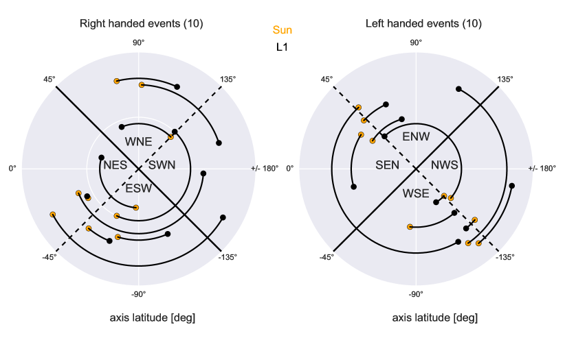
Figure 5: Change in the flux rope clock angle from the Sun to L1, split into right- and left-handed events. The yellow dots represent the flux rope axis orientation at the Sun (the average between the orientations of the PIL and the PEAs), while the black dots indicate the orientation at L1 (taken from the axis orientation resulting from the MVA). Rotations are assumed to be ¡ $180^{\circ}$ , i.e. clockwise and counterclockwise rotations depending on chirality are not considered. Error bars are not included in the plot, but we assume that the error for the solar orientations can be up to $\pm 20^{\circ}$ and for the in situ one can be up to $\pm 45^{\circ}$.

It is also interesting to investigate whether the CME source region location or the crossing distance of the spacecraft along and across the ICME affect whether the intrinsic and in situ flux rope types match. Figure 6 shows the source coordinates of the CMEs, measured as the mid point between the flux rope footpoints. The colors show whether the intrinsic and in situ flux ropes matched or not and the symbols give an estimate of the crossing distance from the ICME axis (Figure 6a) and the ICME nose (Figure 6b). We remind that the crossing distance across the flux rope was estimated through the ratio $\langle|B_{\min}|\rangle/\langle B\rangle$ in the MVA reference system, while the crossing distance along the flux rope was estimated through the location angle (see Section 2.4). It is clear that there is no obvious pattern, regarding either the source location or the crossing distance from the axis and nose of the ICMEs. Nearly all source regions are clustered relatively close to the solar disc centre, within $\pm 30^{\circ}$ both in latitude and longitude. The events with the largest distances from the disc centre are, however, identified as mismatches or intermediate cases.

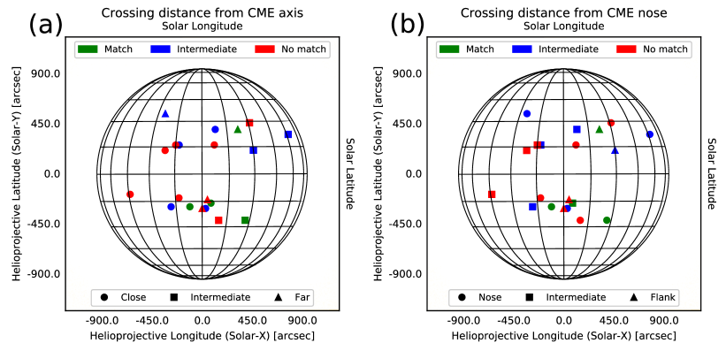
Figure 6: Location of the source regions of the 20 CMEs under analysis. The different colours refer to how the flux rope types match between the Sun and L1: exact match (green), intermediate match (blue), and no match (red). The different symbols refer to the spacecraft crossing distance along and across the ICME. For panel (a), crossing closer to the axis (circles, $\langle|B_{\min}|\rangle/\langle B\rangle$ ¡ 0.2), intermediate crossing (squares, 0.2 ¡ $\langle|B_{\min}|\rangle/\langle B\rangle$ ¡ 0.4), and crossing farther from the axis (triangles, $\langle|B_{\min}|\rangle/\langle B\rangle$ ¿ 0.4). For panel (b), nose crossing (circles, $|\text{L}|$ ¡ $15^{\circ}$), intermediate crossing (squares, $15^{\circ}$ ¡ $|\text{L}|$ ¡ $30^{\circ}$), and crossing closer to the flank (triangles, $|\text{L}|$ ¿ $30^{\circ}$).

4 Discussion and Conclusions

In this work, we have analysed 20 CME events that had a clear and unique connection from the Sun to Earth as determined by heliospheric imaging. We have analysed their magnetic structure (specifically flux rope type) both at the Sun and in situ at the Lagrange L1 point. The analysis of the solar sources was performed following the scheme presented in Palmerio et al. (2017). In particular, several multiwavelength indirect proxies were used to obtain the flux rope helicity sign (chirality), the axis tilt, and the direction of the magnetic field at the central axis, in order to determine the flux rope type of the erupting CME. The in situ flux rope type was determined by visual inspection of magnetic field data and by applying the MVA technique.

One important work towards understanding of the magnetic structure of ICMEs with a flux rope structure and their solar counterparts was performed by Bothmer and Schwenn (1998). The authors estimated the flux rope type of 46 ICMEs and found a unique association for nine ICMEs with quiet-Sun filament eruptions. In eight of the nine cases, they found agreement between the solar and in situ flux rope types, where the intrinsic flux rope configuration was inferred from the orientation of the filament axis and its magnetic polarity, and the heliospheric helicity rule. A more recent study by Savani et al. (2015) studied eight CME events from the Sun to Earth, using the Bothmer and Schwenn (1998) scheme to estimate the intrinsic flux rope configuration, and proved that the initial flux rope structure must be adjusted for cases originating from between two active regions. Indeed, our present study shows that the Palmerio et al. (2017) scheme to determine the intrinsic flux rope type is applicable to several different types of CME eruptions. Our analysis included CMEs originating from a single active region, from pairs of nearby active regions, and from filaments located on the quiet Sun. The scheme succeeded in estimating the intrinsic flux rope type also for CME source regions that did not follow the hemispheric helicity rule. We remark that the chirality has been determined from observations rather than from applying the statistical helicity rule. The proxies that we used and their success rate (i.e., the percentage of the events to which we could apply them) are: arcade skew (90%), S-shaped features (70%), filament characteristics (60%), flare ribbons (55%), and magnetic tongues (15%). We point out that, for the quiet Sun filaments, we were typically able to study filament characteristics only using H$\alpha$, while for active regions filaments, we typically used EUV observations. The flux rope axis orientation at the Sun could by determined both from PIL and PEAs in 65% of cases and from PIL only in rest of the cases.

We found that the flux rope types at the Sun (i.e., the intrinsic flux rope type) and in situ matched only for four (20%) events but, if intermediate cases are considered as a match, then the rate is considerably higher, 11 events (55%). The tendency of the tilt of the flux rope axis at the Sun to be close to $45^{\circ}$ is hence problematic for determining between the eight traditional flux rope categories. As mentioned in Section 3, this trend was noted by Marubashi et al. (2015). There is a tendency for bipolar active regions to emerge with a systematic deviation from the East–West direction, with the leading sunspot being closer to the solar equator. This pattern is known as Joy’s law (Hale et al., 1919). The tilt angle of bipolar sunspot groups (i.e., the line that connects two sunspots), however, tends to have an inclination of $1^{\circ}$–$10^{\circ}$ only due to Joy’s law (e.g., van Driel-Gesztelyi and Green, 2015). This means that the angle of the corresponding PIL tends to be $89^{\circ}$–$80^{\circ}$ tilted to the ecliptic upon emergence. Most of the PILs under analysis were clustered around $45^{\circ}$ tilt, which means that Joy’s law cannot explain such tendency. Since magnetic tongues could be used as a helicity proxy for three events only (out of 14 CMEs originating from a single active region), then it follows that most of the studied active regions were in their decay phase. A possible cause for the PILs to increasingly change their alignment from North–South to Northwest–Southeast (Northeast–Southwest) for right-handed (left-handed) active regions is the Sun’s differential rotation, which progressively acts on the PILs’ tilt angle. This would also hold for active regions that are at the final phase of their decay, which are usually source regions for quite-Sun filament eruptions.

The frequent mismatch in flux rope type between the Sun and Earth suggests significant evolution after the eruption, particularly in terms of flux rope rotation. The comparison of the flux rope axis direction at the Sun and the Earth showed that for 35% of the events that we studied (7 events) the difference between the axis directions at the Sun and in situ was ¿ $90^{\circ}$, with 20% (i.e., 4 events) undergoing over $150^{\circ}$ rotation of their axis. All of the events that experienced a very large difference in the flux rope axis orientation originated from an active region. For the rest of the events (65%; 13 events) the rotation was ¡ $90^{\circ}$, and for 25% of the events (i.e., 5 events) the difference was ¡ $30^{\circ}$. Moreover, the four events that originated from a quiet-Sun filament seemed to rotate ¡ $45^{\circ}$. This is in agreement with Bothmer and Schwenn (1998), that found consistency in the flux rope configuration of erupting quiet-Sun filaments with their in situ counterparts for eight out of nine cases. We therefore suggest that our lower percentage of matches between solar and in situ flux rope types derives from the fact that we considered mostly active region CMEs in our dataset. We also showed that, at least for our relatively small data set, the difference between the axis orientations at the Sun and L1 did not seem to be obviously affected by the CME source location or by the crossing distance along and across the flux rope loop (Figure 6). We remind the reader that, in this analysis, we did not consider the expected sense of rotation dictated by the flux rope chirality, i.e. clockwise (anticlockwise) for right- (left-) handed events. In fact, if we consider the smallest angle between the solar and in situ flux rope orientations, then only ten events (50%) seem to follow the sense of rotation expected from their chirality. This may either be because the remaining ten CMEs actually rotated in the opposite sense or that there was an external factor that counteracted the expected sense of rotation.

However, it is important to remark that the resulting flux rope orientation in situ may depend on the fitting technique. Al-Haddad et al. (2013) analysed 59 ICMEs using four different reconstruction or fitting methods, and found that for one event only all four methods found an orientation of the ICME axis within $\pm 45^{\circ}$. Reconstructions done with different techniques usually disagree, and that has to be taken into account when comparing solar and in situ orientations, especially when considering the sense of rotation of the axis for the low rotation cases. If we consider, e.g., only the cases that present a ¿ $45^{\circ}$ angular difference (i.e., 11 events in total), then four (five) right-handed (left-handed) flux ropes seemed to rotate anticlockwise and two (zero) clockwise. The left-handed events, hence, seem all to follow the expected sense of rotation if the analysis is restricted to the large rotation cases.

It is noteworthy that the direct comparison between intrinsic and in situ flux rope types can be performed only for a fraction of all CME–ICME pairs. As discussed in Section 2, we considered 47 candidates from the LINKCAT catalogue and ended up with only 12 events. The problems are related to (1) correctly connecting the CME–ICME pair, (2) excluding interacting events, and (3) the requirement for the relevant observations to be sufficiently clear both at the Sun and in situ in order to estimate the flux rope type. In particular, many ICMEs do not show clear enough rotation of the field to determine the flux rope type. At the Sun, some CMEs may be so-called stealth CMEs (e.g., Robbrecht et al., 2009; Kilpua et al., 2014; Nitta and Mulligan, 2017), i.e. they lack obvious disk signatures, or have curved PEAs and/or PIL so reliable determination of the axis orientation is not possible. However, the cases for which determination of the intrinsic and in situ flux rope types is possible are often geoeffective, as they show clear magnetic field enhancements and organized rotation of the magnetic field. In addition, as remarked in the Introduction, one important point to keep in mind for real-time space weather forecasts is that it is often difficult to predict if an erupting CME would impact Earth at all. Hence, a further investigation to study the applicability of the methods described in this article for forecasting would require to start at the Sun without first identifying CME–ICME pairs.

As already mentioned in the Introduction, determination of the intrinsic flux rope type is a crucial step in space weather forecasting (as the input to different models), and as showed in this paper, in a fraction of cases it gives a good estimate of the flux rope magnetic structure at L1. Our results, however, strongly highlight the importance of capturing the amount of rotation and/or distortion that the flux rope experiences in the corona and in interplanetary space. This was stated already in the work by Savani et al. (2015), that highlights the importance of including evolutionary estimates of CMEs from remote sensing for space weather forecasts. The flux rope axis direction in situ can be, e.g., estimated by considering coronagraph data in addition to solar disc observations (Savani et al., 2015). Concerning flux rope rotations, in fact, several studies suggest that the most dramatic rotation occurs during the first few solar radii of a CME’s propagation (e.g., Vourlidas et al., 2011; Isavnin et al., 2014; Kay et al., 2016). Indeed, rotation can also occur even during the eruption (e.g., Green et al., 2007; Lynch et al., 2009; Bemporad et al., 2011; Thompson et al., 2012).

Finally, we remark that in situ data are one-dimensional and that a single spacecraft’s trajectory through a CME may not reflect the global shape and orientation of the flux rope. The flux rope type that is seen at Earth may depend on where the spacecraft crosses the ICME (i.e. the crossing distance from the ICME axis, named the impact parameter, and/or from the ICME nose) and on local distortions that might be present within an ICME. In terms of the latter, Bothmer and Mrotzek (2017) recently demonstrated that kinks present in the CME source region seem to be reflected in the erupting flux rope during its expansion and propagation. Owens et al. (2017) also showed that CMEs cease to be coherent magnetohydrodynamic structures within 0.3 AU of the Sun, and that their appearance beyond this distance is that of a dust cloud. This means that local deformations that may arise during the CME propagation do not propagate throughout the whole CME body. Nevertheless, the space weather effects at Earth depend strongly on the magnetic structure that is measured at L1, meaning that a significant step towards the improvement of current space weather forecasting capabilities is the prediction of the flux rope axis rotation (whether proper or apparent) during propagation. Other important factors to take into account for future space weather predictions are the crossing location, both along and across the flux rope, and eventual local distortions of the CME body.

Sources of Data and Supplementary Material

Catalogues:
 
LINKCAT, doi:10.6084/m9.figshare.4588330.v2,
https://doi.org/10.6084/m9.figshare.4588330.v2
ARRCAT, doi:10.6084/m9.figshare.4588324.v1,
https://doi.org/10.6084/m9.figshare.4588324.v1
 
ICME Lists:
 
Near-Earth Interplanetary Coronal Mass Ejections List, Richardson, I., and Cane, H.,
http://www.srl.caltech.edu/ACE/ASC/DATA/level3/icmetable2.htm
Wind ICME List, Nieves-Chinchilla, T., et al.,
https://wind.nasa.gov/ICMEindex.php

References

- Al-Haddad et al. (2013) Al-Haddad, N., T. Nieves-Chinchilla, N. P. Savani, C. Möstl, K. Marubashi, M. A. Hidalgo, I. I. Roussev, S. Poedts, and C. J. Farrugia (2013), Magnetic Field Configuration Models and Reconstruction Methods for Interplanetary Coronal Mass Ejections, Solar Phys., 284, 129–149, 10.1007/s11207-013-0244-5.
- Antiochos et al. (1999) Antiochos, S. K., C. R. DeVore, and J. A. Klimchuk (1999), A Model for Solar Coronal Mass Ejections, Astrophys. J., 510, 485–493, 10.1086/306563.
- Bemporad et al. (2011) Bemporad, A., M. Mierla, and D. Tripathi (2011), Rotation of an erupting filament observed by the STEREO EUVI and COR1 instruments, Astron. Astrophys., 531, A147, 10.1051/0004-6361/201016297.
- Berghmans et al. (2006) Berghmans, D., J. F. Hochedez, J. M. Defise, J. H. Lecat, B. Nicula, V. Slemzin, G. Lawrence, A. C. Katsyiannis, R. van der Linden, A. Zhukov, F. Clette, P. Rochus, E. Mazy, T. Thibert, P. Nicolosi, M.-G. Pelizzo, and U. Schühle (2006), SWAP onboard PROBA 2, a new EUV imager for solar monitoring, Advances in Space Research, 38, 1807–1811, 10.1016/j.asr.2005.03.070.
- Bobra et al. (2014) Bobra, M. G., X. Sun, J. T. Hoeksema, M. Turmon, Y. Liu, K. Hayashi, G. Barnes, and K. D. Leka (2014), The Helioseismic and Magnetic Imager (HMI) Vector Magnetic Field Pipeline: SHARPs – Space-Weather HMI Active Region Patches, Solar Phys., 289, 3549–3578, 10.1007/s11207-014-0529-3.
- Bothmer and Mrotzek (2017) Bothmer, V., and N. Mrotzek (2017), Comparison of CME and ICME Structures Derived from Remote-Sensing and In Situ Observations, Solar Phys., 292, 157, 10.1007/s11207-017-1171-7.
- Bothmer and Schwenn (1998) Bothmer, V., and R. Schwenn (1998), The structure and origin of magnetic clouds in the solar wind, Ann. Geophys., 16, 1–24, 10.1007/s00585-997-0001-x.
- Brueckner et al. (1995) Brueckner, G. E., R. A. Howard, M. J. Koomen, C. M. Korendyke, D. J. Michels, J. D. Moses, D. G. Socker, K. P. Dere, P. L. Lamy, A. Llebaria, M. V. Bout, R. Schwenn, G. M. Simnett, D. K. Bedford, and C. J. Eyles (1995), The Large Angle Spectroscopic Coronagraph (LASCO), Solar Phys., 162, 357–402, 10.1007/BF00733434.
- Burlaga et al. (1981) Burlaga, L., E. Sittler, F. Mariani, and R. Schwenn (1981), Magnetic loop behind an interplanetary shock - Voyager, Helios, and IMP 8 observations, J. Geophys. Res., 86, 6673–6684, 10.1029/JA086iA08p06673.
- Burlaga et al. (2002) Burlaga, L. F., S. P. Plunkett, and O. C. St. Cyr (2002), Successive CMEs and complex ejecta, J. Geophys. Res. Space Physics, 107, 1266, 10.1029/2001JA000255.
- Cane et al. (1997) Cane, H. V., I. G. Richardson, and G. Wibberenz (1997), Helios 1 and 2 observations of particle decreases, ejecta, and magnetic clouds, J. Geophys. Res., 102, 7075–7086, 10.1029/97JA00149.
- Canfield et al. (1999) Canfield, R. C., H. S. Hudson, and D. E. McKenzie (1999), Sigmoidal morphology and eruptive solar activity, Geophys. Res. Lett., 26, 627–630, 10.1029/1999GL900105.
- Chae (2000) Chae, J. (2000), The Magnetic Helicity Sign of Filament Chirality, Astrophys. J. Lett., 540, L115–L118, 10.1086/312880.
- Cho et al. (2013) Cho, K.-S., S.-H. Park, K. Marubashi, N. Gopalswamy, S. Akiyama, S. Yashiro, R.-S. Kim, and E.-K. Lim (2013), Comparison of Helicity Signs in Interplanetary CMEs and Their Solar Source Regions, Solar Phys., 284, 105–127, 10.1007/s11207-013-0224-9.
- Dasso et al. (2007) Dasso, S., M. S. Nakwacki, P. Démoulin, and C. H. Mandrini (2007), Progressive Transformation of a Flux Rope to an ICME. Comparative Analysis Using the Direct and Fitted Expansion Methods, Solar Phys., 244, 115–137, 10.1007/s11207-007-9034-2.
- Davies et al. (2012) Davies, J. A., R. A. Harrison, C. H. Perry, C. Möstl, N. Lugaz, T. Rollett, C. J. Davis, S. R. Crothers, M. Temmer, C. J. Eyles, and N. P. Savani (2012), A Self-similar Expansion Model for Use in Solar Wind Transient Propagation Studies, Astrophys. J., 750, 23, 10.1088/0004-637X/750/1/23.
- Démoulin and Dasso (2009) Démoulin, P., and S. Dasso (2009), Magnetic cloud models with bent and oblate cross-section boundaries, Astron. Astrophys., 507, 969–980, 10.1051/0004-6361/200912645.
- Démoulin et al. (1996) Démoulin, P., E. R. Priest, and D. P. Lonie (1996), Three-dimensional magnetic reconnection without null points 2. Application to twisted flux tubes, J. Geophys. Res., 101, 7631–7646, 10.1029/95JA03558.
- Domingo et al. (1995) Domingo, V., B. Fleck, and A. I. Poland (1995), The SOHO Mission: an Overview, Solar Phys., 162, 1–37, 10.1007/BF00733425.
- Dungey (1961) Dungey, J. W. (1961), Interplanetary Magnetic Field and the Auroral Zones, Phys. Rev. Lett., 6, 47–48, 10.1103/PhysRevLett.6.47.
- Eyles et al. (2009) Eyles, C. J., R. A. Harrison, C. J. Davis, N. R. Waltham, B. M. Shaughnessy, H. C. A. Mapson-Menard, D. Bewsher, S. R. Crothers, J. A. Davies, G. M. Simnett, R. A. Howard, J. D. Moses, J. S. Newmark, D. G. Socker, J.-P. Halain, J.-M. Defise, E. Mazy, and P. Rochus (2009), The Heliospheric Imagers Onboard the STEREO Mission, Solar Phys., 254, 387–445, 10.1007/s11207-008-9299-0.
- Fan and Gibson (2003) Fan, Y., and S. E. Gibson (2003), The Emergence of a Twisted Magnetic Flux Tube into a Preexisting Coronal Arcade, Astrophys. J. Lett., 589, L105–L108, 10.1086/375834.
- Golub et al. (2007) Golub, L., E. Deluca, G. Austin, J. Bookbinder, D. Caldwell, P. Cheimets, J. Cirtain, M. Cosmo, P. Reid, A. Sette, M. Weber, T. Sakao, R. Kano, K. Shibasaki, H. Hara, S. Tsuneta, K. Kumagai, T. Tamura, M. Shimojo, J. McCracken, J. Carpenter, H. Haight, R. Siler, E. Wright, J. Tucker, H. Rutledge, M. Barbera, G. Peres, and S. Varisco (2007), The X-Ray Telescope (XRT) for the Hinode Mission, Solar Phys., 243, 63–86, 10.1007/s11207-007-0182-1.
- Gonzalez and Tsurutani (1987) Gonzalez, W. D., and B. T. Tsurutani (1987), Criteria of interplanetary parameters causing intense magnetic storms (Dst of less than -100 nT), Planet. Space Sci., 35, 1101–1109, 10.1016/0032-0633(87)90015-8.
- Gonzalez et al. (1994) Gonzalez, W. D., J. A. Joselyn, Y. Kamide, H. W. Kroehl, G. Rostoker, B. T. Tsurutani, and V. M. Vasyliunas (1994), What is a geomagnetic storm?, J. Geophys. Res., 99, 5771–5792, 10.1029/93JA02867.
- Gosling (1990) Gosling, J. T. (1990), Coronal mass ejections and magnetic flux ropes in interplanetary space, Geophys. Monogr. Ser., 58, 343–364.
- Gosling et al. (1991) Gosling, J. T., D. J. McComas, J. L. Phillips, and S. J. Bame (1991), Geomagnetic activity associated with earth passage of interplanetary shock disturbances and coronal mass ejections, J. Geophys. Res., 96, 7831–7839, 10.1029/91JA00316.
- Green et al. (2007) Green, L. M., B. Kliem, T. Török, L. van Driel-Gesztelyi, and G. D. R. Attrill (2007), Transient Coronal Sigmoids and Rotating Erupting Flux Ropes, Solar Phys., 246, 365–391, 10.1007/s11207-007-9061-z.
- Gulisano et al. (2007) Gulisano, A. M., S. Dasso, C. H. Mandrini, and P. Démoulin (2007), Estimation of the bias of the Minimum Variance technique in the determination of magnetic clouds global quantities and orientation, Advances in Space Research, 40, 1881–1890, 10.1016/j.asr.2007.09.001.
- Hale et al. (1919) Hale, G. E., F. Ellerman, S. B. Nicholson, and A. H. Joy (1919), The Magnetic Polarity of Sun-Spots, Astrophys. J., 49, 153, 10.1086/142452.
- Harra et al. (2007) Harra, L. K., N. U. Crooker, C. H. Mandrini, L. van Driel-Gesztelyi, S. Dasso, J. Wang, H. Elliott, G. Attrill, B. V. Jackson, and M. M. Bisi (2007), How Does Large Flaring Activity from the Same Active Region Produce Oppositely Directed Magnetic Clouds?, Solar Phys., 244, 95–114, 10.1007/s11207-007-9002-x.
- Howard et al. (2008) Howard, R. A., J. D. Moses, A. Vourlidas, J. S. Newmark, D. G. Socker, S. P. Plunkett, C. M. Korendyke, J. W. Cook, A. Hurley, J. M. Davila, W. T. Thompson, O. C. St Cyr, E. Mentzell, K. Mehalick, J. R. Lemen, J. P. Wuelser, D. W. Duncan, T. D. Tarbell, C. J. Wolfson, A. Moore, R. A. Harrison, N. R. Waltham, J. Lang, C. J. Davis, C. J. Eyles, H. Mapson-Menard, G. M. Simnett, J. P. Halain, J. M. Defise, E. Mazy, P. Rochus, R. Mercier, M. F. Ravet, F. Delmotte, F. Auchere, J. P. Delaboudiniere, V. Bothmer, W. Deutsch, D. Wang, N. Rich, S. Cooper, V. Stephens, G. Maahs, R. Baugh, D. McMullin, and T. Carter (2008), Sun Earth Connection Coronal and Heliospheric Investigation (SECCHI), Space Sci. Rev., 136, 67–115, 10.1007/s11214-008-9341-4.
- Hu et al. (2014) Hu, Q., J. Qiu, B. Dasgupta, A. Khare, and G. M. Webb (2014), Structures of Interplanetary Magnetic Flux Ropes and Comparison with Their Solar Sources, Astrophys. J., 793, 53, 10.1088/0004-637X/793/1/53.
- Huttunen and Koskinen (2004) Huttunen, K., and H. Koskinen (2004), Importance of post-shock streams and sheath region as drivers of intense magnetospheric storms and high-latitude activity, Ann. Geophys., 22, 1729–1738, 10.5194/angeo-22-1729-2004.
- Huttunen et al. (2002) Huttunen, K. E. J., H. E. J. Koskinen, and R. Schwenn (2002), Variability of magnetospheric storms driven by different solar wind perturbations, Journal of Geophysical Research (Space Physics), 107, 1121, 10.1029/2001JA900171.
- Huttunen et al. (2005) Huttunen, K. E. J., R. Schwenn, V. Bothmer, and H. E. J. Koskinen (2005), Properties and geoeffectiveness of magnetic clouds in the rising, maximum and early declining phases of solar cycle 23, Ann. Geophys., 23, 625–641, 10.5194/angeo-23-625-2005.
- Isavnin et al. (2013) Isavnin, A., A. Vourlidas, and E. K. J. Kilpua (2013), Three-Dimensional Evolution of Erupted Flux Ropes from the Sun (2–20 R⊙) to 1 AU, Solar Phys., 284, 203–215, 10.1007/s11207-012-0214-3.
- Isavnin et al. (2014) Isavnin, A., A. Vourlidas, and E. K. J. Kilpua (2014), Three-Dimensional Evolution of Flux-Rope CMEs and Its Relation to the Local Orientation of the Heliospheric Current Sheet, Solar Phys., 289, 2141–2156, 10.1007/s11207-013-0468-4.
- James et al. (2017) James, A. W., L. M. Green, E. Palmerio, G. Valori, H. A. S. Reid, D. Baker, D. H. Brooks, L. van Driel-Gesztelyi, and E. K. J. Kilpua (2017), On-Disc Observations of Flux Rope Formation Prior to Its Eruption, Solar Phys., 292, 71, 10.1007/s11207-017-1093-4.
- Janvier et al. (2013) Janvier, M., P. Démoulin, and S. Dasso (2013), Global axis shape of magnetic clouds deduced from the distribution of their local axis orientation, Astron. Astrophys., 556, A50, 10.1051/0004-6361/201321442.
- Jian et al. (2006) Jian, L., C. T. Russell, J. G. Luhmann, and R. M. Skoug (2006), Properties of Interplanetary Coronal Mass Ejections at One AU During 1995 2004, Solar Phys., 239, 393–436, 10.1007/s11207-006-0133-2.
- Kaiser et al. (2008) Kaiser, M. L., T. A. Kucera, J. M. Davila, O. C. St. Cyr, M. Guhathakurta, and E. Christian (2008), The STEREO Mission: An Introduction, Space Sci. Rev., 136, 5–16, 10.1007/s11214-007-9277-0.
- Kay et al. (2013) Kay, C., M. Opher, and R. M. Evans (2013), Forecasting a Coronal Mass Ejection’s Altered Trajectory: ForeCAT, Astrophys. J., 775, 5, 10.1088/0004-637X/775/1/5.
- Kay et al. (2016) Kay, C., M. Opher, R. C. Colaninno, and A. Vourlidas (2016), Using ForeCAT Deflections and Rotations to Constrain the Early Evolution of CMEs, Astrophys. J., 827, 70, 10.3847/0004-637X/827/1/70.
- Kay et al. (2017) Kay, C., N. Gopalswamy, A. Reinard, and M. Opher (2017), Predicting the Magnetic Field of Earth-impacting CMEs, Astrophys. J., 835, 117, 10.3847/1538-4357/835/2/117.
- Kilpua et al. (2017a) Kilpua, E., H. E. J. Koskinen, and T. I. Pulkkinen (2017a), Coronal mass ejections and their sheath regions in interplanetary space, Living Reviews in Solar Physics, 14, 5, 10.1007/s41116-017-0009-6.
- Kilpua et al. (2009) Kilpua, E. K. J., P. C. Liewer, C. Farrugia, J. G. Luhmann, C. Möstl, Y. Li, Y. Liu, B. J. Lynch, C. T. Russell, A. Vourlidas, M. H. Acuna, A. B. Galvin, D. Larson, and J. A. Sauvaud (2009), Multispacecraft Observations of Magnetic Clouds and Their Solar Origins between 19 and 23 May 2007, Solar Phys., 254, 325–344, 10.1007/s11207-008-9300-y.
- Kilpua et al. (2011) Kilpua, E. K. J., L. K. Jian, Y. Li, J. G. Luhmann, and C. T. Russell (2011), Multipoint ICME encounters: Pre-STEREO and STEREO observations, J. Atmos. Solar-Terr. Phys., 73, 1228–1241, 10.1016/j.jastp.2010.10.012.
- Kilpua et al. (2014) Kilpua, E. K. J., M. Mierla, A. N. Zhukov, L. Rodriguez, A. Vourlidas, and B. Wood (2014), Solar Sources of Interplanetary Coronal Mass Ejections During the Solar Cycle 23/24 Minimum, Solar Phys., 289, 3773–3797, 10.1007/s11207-014-0552-4.
- Kilpua et al. (2017b) Kilpua, E. K. J., A. Balogh, R. von Steiger, and Y. D. Liu (2017b), Geoeffective Properties of Solar Transients and Stream Interaction Regions, Space Sci. Rev., 10.1007/s11214-017-0411-3.
- Kliem and Török (2006) Kliem, B., and T. Török (2006), Torus Instability, Phys. Rev. Lett., 96(25), 255002, 10.1103/PhysRevLett.96.255002.
- Kosugi et al. (2007) Kosugi, T., K. Matsuzaki, T. Sakao, T. Shimizu, Y. Sone, S. Tachikawa, T. Hashimoto, K. Minesugi, A. Ohnishi, T. Yamada, S. Tsuneta, H. Hara, K. Ichimoto, Y. Suematsu, M. Shimojo, T. Watanabe, S. Shimada, J. M. Davis, L. D. Hill, J. K. Owens, A. M. Title, J. L. Culhane, L. K. Harra, G. A. Doschek, and L. Golub (2007), The Hinode (Solar-B) Mission: An Overview, Solar Phys., 243, 3–17, 10.1007/s11207-007-9014-6.
- Kubicka et al. (2016) Kubicka, M., C. Möstl, T. Amerstorfer, P. D. Boakes, L. Feng, J. P. Eastwood, and O. Törmänen (2016), Prediction of Geomagnetic Storm Strength from Inner Heliospheric In Situ Observations, Astrophys. J., 833, 255, 10.3847/1538-4357/833/2/255.
- Leamon et al. (2004) Leamon, R. J., R. C. Canfield, S. L. Jones, K. Lambkin, B. J. Lundberg, and A. A. Pevtsov (2004), Helicity of magnetic clouds and their associated active regions, Journal of Geophysical Research (Space Physics), 109, A05106, 10.1029/2003JA010324.
- Lemen et al. (2012) Lemen, J. R., A. M. Title, D. J. Akin, P. F. Boerner, C. Chou, J. F. Drake, D. W. Duncan, C. G. Edwards, F. M. Friedlaender, G. F. Heyman, N. E. Hurlburt, N. L. Katz, G. D. Kushner, M. Levay, R. W. Lindgren, D. P. Mathur, E. L. McFeaters, S. Mitchell, R. A. Rehse, C. J. Schrijver, L. A. Springer, R. A. Stern, T. D. Tarbell, J.-P. Wuelser, C. J. Wolfson, C. Yanari, J. A. Bookbinder, P. N. Cheimets, D. Caldwell, E. E. Deluca, R. Gates, L. Golub, S. Park, W. A. Podgorski, R. I. Bush, P. H. Scherrer, M. A. Gummin, P. Smith, G. Auker, P. Jerram, P. Pool, R. Soufli, D. L. Windt, S. Beardsley, M. Clapp, J. Lang, and N. Waltham (2012), The Atmospheric Imaging Assembly (AIA) on the Solar Dynamics Observatory (SDO), Solar Phys., 275, 17–40, 10.1007/s11207-011-9776-8.
- Lepping and Behannon (1980) Lepping, R. P., and K. W. Behannon (1980), Magnetic field directional discontinuities. I - Minimum variance errors, J. Geophys. Res., 85, 4695–4703, 10.1029/JA085iA09p04695.
- Lepping et al. (1995) Lepping, R. P., M. H. Acũna, L. F. Burlaga, W. M. Farrell, J. A. Slavin, K. H. Schatten, F. Mariani, N. F. Ness, F. M. Neubauer, Y. C. Whang, J. B. Byrnes, R. S. Kennon, P. V. Panetta, J. Scheifele, and E. M. Worley (1995), The Wind Magnetic Field Investigation, Space Sci. Rev., 71, 207–229, 10.1007/BF00751330.
- Liu et al. (2008) Liu, Y., J. G. Luhmann, K. E. J. Huttunen, R. P. Lin, S. D. Bale, C. T. Russell, and A. B. Galvin (2008), Reconstruction of the 2007 May 22 Magnetic Cloud: How Much Can We Trust the Flux-Rope Geometry of CMEs?, Astrophys. J. Lett., 677, L133, 10.1086/587839.
- López Fuentes et al. (2000) López Fuentes, M. C., P. Demoulin, C. H. Mandrini, and L. van Driel-Gesztelyi (2000), The Counterkink Rotation of a Non-Hale Active Region, Astrophys. J., 544, 540–549, 10.1086/317180.
- Lugaz et al. (2012) Lugaz, N., C. J. Farrugia, J. A. Davies, C. Möstl, C. J. Davis, I. I. Roussev, and M. Temmer (2012), The Deflection of the Two Interacting Coronal Mass Ejections of 2010 May 23-24 as Revealed by Combined in Situ Measurements and Heliospheric Imaging, Astrophys. J., 759, 68, 10.1088/0004-637X/759/1/68.
- Luoni et al. (2011) Luoni, M. L., P. Démoulin, C. H. Mandrini, and L. van Driel-Gesztelyi (2011), Twisted Flux Tube Emergence Evidenced in Longitudinal Magnetograms: Magnetic Tongues, Solar Phys., 270, 45–74, 10.1007/s11207-011-9731-8.
- Lynch et al. (2009) Lynch, B. J., S. K. Antiochos, Y. Li, J. G. Luhmann, and C. R. DeVore (2009), Rotation of Coronal Mass Ejections during Eruption, Astrophys. J., 697, 1918–1927, 10.1088/0004-637X/697/2/1918.
- Manchester et al. (2017) Manchester, W., E. K. J. Kilpua, Y. D. Liu, N. Lugaz, P. Riley, T. Török, and B. Vršnak (2017), The Physical Processes of CME/ICME Evolution, Space Sci. Rev., 10.1007/s11214-017-0394-0.
- Martin and McAllister (1996) Martin, S. F., and A. H. McAllister (1996), The Skew of X-ray Coronal Loops Overlying H alpha Filaments, in IAU Colloq. 153: Magnetodynamic Phenomena in the Solar Atmosphere - Prototypes of Stellar Magnetic Activity, edited by Y. Uchida, T. Kosugi, and H. S. Hudson, p. 497.
- Martin et al. (1994) Martin, S. F., R. Bilimoria, and P. W. Tracadas (1994), Magnetic field configurations basic to filament channels and filaments, in Mathematical and Physical Sciences, Proceedings of the NATO Advanced Research Workshop, NATO Advanced Science Institutes (ASI) Series C, vol. 433, edited by R. J. Rutten and C. J. Schrijver, p. 303.
- Martin et al. (2012) Martin, S. F., O. Panasenco, M. A. Berger, O. Engvold, Y. Lin, A. A. Pevtsov, and N. Srivastava (2012), The Build-Up to Eruptive Solar Events Viewed as the Development of Chiral Systems, in Second ATST-EAST Meeting: Magnetic Fields from the Photosphere to the Corona., Astron. Soc. Pacific C.S., vol. 463, edited by T. R. Rimmele, A. Tritschler, F. Wöger, M. Collados Vera, H. Socas-Navarro, R. Schlichenmaier, M. Carlsson, T. Berger, A. Cadavid, P. R. Gilbert, P. R. Goode, and M. Knölker, p. 157.
- Marubashi et al. (2015) Marubashi, K., S. Akiyama, S. Yashiro, N. Gopalswamy, K.-S. Cho, and Y.-D. Park (2015), Geometrical Relationship Between Interplanetary Flux Ropes and Their Solar Sources, Solar Phys., 290, 1371–1397, 10.1007/s11207-015-0681-4.
- Mays et al. (2015) Mays, M. L., B. J. Thompson, L. K. Jian, R. C. Colaninno, D. Odstrcil, C. Möstl, M. Temmer, N. P. Savani, G. Collinson, A. Taktakishvili, P. J. MacNeice, and Y. Zheng (2015), Propagation of the 7 January 2014 CME and Resulting Geomagnetic Non-event, Astrophys. J., 812, 145, 10.1088/0004-637X/812/2/145.
- McAllister et al. (1998) McAllister, A. H., A. J. Hundhausen, D. Mackay, and E. Priest (1998), The Skew of Polar Crown X-ray Arcades, in IAU Colloq. 167: New Perspectives on Solar Prominences, Astron. Soc. Pacific C.S., vol. 150, edited by D. F. Webb, B. Schmieder, and D. M. Rust, p. 430.
- McAllister et al. (2001) McAllister, A. H., S. F. Martin, N. U. Crooker, R. P. Lepping, and R. J. Fitzenreiter (2001), A test of real-time prediction of magnetic cloud topology and geomagnetic storm occurrence from solar signatures, J. Geophys. Res., 106, 29,185–29,194, 10.1029/2000JA000032.
- Moore et al. (2001) Moore, R. L., A. C. Sterling, H. S. Hudson, and J. R. Lemen (2001), Onset of the Magnetic Explosion in Solar Flares and Coronal Mass Ejections, Astrophys. J., 552, 833–848, 10.1086/320559.
- Möstl et al. (2008) Möstl, C., C. Miklenic, C. J. Farrugia, M. Temmer, A. Veronig, A. B. Galvin, B. Vršnak, and H. K. Biernat (2008), Two-spacecraft reconstruction of a magnetic cloud and comparison to its solar source, Ann. Geophys., 26, 3139–3152, 10.5194/angeo-26-3139-2008.
- Möstl et al. (2009) Möstl, C., C. J. Farrugia, C. Miklenic, M. Temmer, A. B. Galvin, J. G. Luhmann, E. K. J. Kilpua, M. Leitner, T. Nieves-Chinchilla, A. Veronig, and H. K. Biernat (2009), Multispacecraft recovery of a magnetic cloud and its origin from magnetic reconnection on the Sun, Journal of Geophysical Research (Space Physics), 114, A04102, 10.1029/2008JA013657.
- Möstl et al. (2014) Möstl, C., K. Amla, J. R. Hall, P. C. Liewer, E. M. De Jong, R. C. Colaninno, A. M. Veronig, T. Rollett, M. Temmer, V. Peinhart, J. A. Davies, N. Lugaz, Y. D. Liu, C. J. Farrugia, J. G. Luhmann, B. Vršnak, R. A. Harrison, and A. B. Galvin (2014), Connecting Speeds, Directions and Arrival Times of 22 Coronal Mass Ejections from the Sun to 1 AU, Astrophys. J., 787, 119, 10.1088/0004-637X/787/2/119.
- Möstl et al. (2017) Möstl, C., A. Isavnin, P. D. Boakes, E. K. J. Kilpua, J. A. Davies, R. A. Harrison, D. Barnes, V. Krupar, J. P. Eastwood, S. W. Good, R. J. Forsyth, V. Bothmer, M. A. Reiss, T. Amerstorfer, R. M. Winslow, B. J. Anderson, L. C. Philpott, L. Rodriguez, A. P. Rouillard, P. Gallagher, T. Nieves-Chinchilla, and T. L. Zhang (2017), Modeling observations of solar coronal mass ejections with heliospheric imagers verified with the Heliophysics System Observatory, Space Weather, 15, 955–970, 10.1002/2017SW001614.
- Möstl et al. (2018) Möstl, C., T. Amerstorfer, E. Palmerio, A. Isavnin, C. J. Farrugia, C. Lowder, R. M. Winslow, J. M. Donnerer, E. K. J. Kilpua, P. D. Boakes (2018), Forward modeling of coronal mass ejection flux ropes in the inner heliosphere with 3DCORE, Space Weather, 16, in press. 10.1002/2017SW001735.
- Mulligan et al. (1998) Mulligan, T., C. T. Russell, and J. G. Luhmann (1998), Solar cycle evolution of the structure of magnetic clouds in the inner heliosphere, Geophys. Res. Lett., 25, 2959–2962, 10.1029/98GL01302.
- Nitta and Mulligan (2017) Nitta, N. V., and T. Mulligan (2017), Earth-Affecting Coronal Mass Ejections Without Obvious Low Coronal Signatures, Solar Phys., 292, 125, 10.1007/s11207-017-1147-7.
- Odstrcil and Pizzo (1999) Odstrcil, D., and V. J. Pizzo (1999), Distortion of the interplanetary magnetic field by three-dimensional propagation of coronal mass ejections in a structured solar wind, J. Geophys. Res., 104, 28,225–28,240, 10.1029/1999JA900319.
- Ogilvie et al. (1995) Ogilvie, K. W., D. J. Chornay, R. J. Fritzenreiter, F. Hunsaker, J. Keller, J. Lobell, G. Miller, J. D. Scudder, E. C. Sittler, Jr., R. B. Torbert, D. Bodet, G. Needell, A. J. Lazarus, J. T. Steinberg, J. H. Tappan, A. Mavretic, and E. Gergin (1995), SWE, A Comprehensive Plasma Instrument for the Wind Spacecraft, Space Sci. Rev., 71, 55–77, 10.1007/BF00751326.
- Owens et al. (2012) Owens, M. J., P. Démoulin, N. P. Savani, B. Lavraud, and A. Ruffenach (2012), Implications of Non-cylindrical Flux Ropes for Magnetic Cloud Reconstruction Techniques and the Interpretation of Double Flux Rope Events, Solar Phys., 278, 435–446, 10.1007/s11207-012-9939-2.
- Owens et al. (2017) Owens, M. J., M. Lockwood, and L. A. Barnard (2017), Coronal mass ejections are not coherent magnetohydrodynamic structures, Scientific Reports, 7, 4152, 10.1038/s41598-017-04546-3.
- Pal et al. (2017) Pal, S., N. Gopalswamy, D. Nandy, S. Akiyama, S. Yashiro, P. Makela, and H. Xie (2017), A Sun-to-Earth Analysis of Magnetic Helicity of the 2013 March 17–18 Interplanetary Coronal Mass Ejection, Astrophys. J., 851, 123, 10.3847/1538-4357/aa9983.
- Palmerio et al. (2017) Palmerio, E., E. K. J. Kilpua, A. W. James, L. M. Green, J. Pomoell, A. Isavnin, and G. Valori (2017), Determining the Intrinsic CME Flux Rope Type Using Remote-sensing Solar Disk Observations, Solar Phys., 292, 39, 10.1007/s11207-017-1063-x.
- Pesnell et al. (2012) Pesnell, W. D., B. J. Thompson, and P. C. Chamberlin (2012), The Solar Dynamics Observatory (SDO), Solar Phys., 275, 3–15, 10.1007/s11207-011-9841-3.
- Pevtsov and Balasubramaniam (2003) Pevtsov, A. A., and K. S. Balasubramaniam (2003), Helicity patterns on the sun, Adv. Space Res., 32, 1867–1874, 10.1016/S0273-1177(03)90620-X.
- Pevtsov et al. (2014) Pevtsov, A. A., M. A. Berger, A. Nindos, A. A. Norton, and L. van Driel-Gesztelyi (2014), Magnetic Helicity, Tilt, and Twist, Space Sci. Rev., 186, 285–324, 10.1007/s11214-014-0082-2.
- Pulkkinen (2007) Pulkkinen, T. (2007), Space Weather: Terrestrial Perspective, Living Rev. Sol. Phys., 4, 1, 10.12942/lrsp-2007-1.
- Qiu et al. (2007) Qiu, J., Q. Hu, T. A. Howard, and V. B. Yurchyshyn (2007), On the Magnetic Flux Budget in Low-Corona Magnetic Reconnection and Interplanetary Coronal Mass Ejections, Astrophys. J., 659, 758–772, 10.1086/512060.
- Richardson and Cane (2004) Richardson, I. G., and H. V. Cane (2004), The fraction of interplanetary coronal mass ejections that are magnetic clouds: Evidence for a solar cycle variation, Geophys. Res. Lett., 31, L18804, 10.1029/2004GL020958.
- Richardson and Cane (2012) Richardson, I. G., and H. V. Cane (2012), Solar wind drivers of geomagnetic storms during more than four solar cycles, Journal of Space Weather and Space Climate, 2(27), A01, 10.1051/swsc/2012001.
- Robbrecht et al. (2009) Robbrecht, E., S. Patsourakos, and A. Vourlidas (2009), No Trace Left Behind: STEREO Observation of a Coronal Mass Ejection Without Low Coronal Signatures, Astrophys. J., 701, 283–291, 10.1088/0004-637X/701/1/283.
- Rodriguez et al. (2016) Rodriguez, L., J. J. Masías-Meza, S. Dasso, P. Démoulin, A. N. Zhukov, A. M. Gulisano, M. Mierla, E. Kilpua, M. West, D. Lacatus, A. Paraschiv, and M. Janvier (2016), Typical Profiles and Distributions of Plasma and Magnetic Field Parameters in Magnetic Clouds at 1 AU, Solar Phys., 291, 2145–2163, 10.1007/s11207-016-0955-5.
- Ruffenach et al. (2012) Ruffenach, A., B. Lavraud, M. J. Owens, J.-A. Sauvaud, N. P. Savani, A. P. Rouillard, P. Démoulin, C. Foullon, A. Opitz, A. Fedorov, C. J. Jacquey, V. Génot, P. Louarn, J. G. Luhmann, C. T. Russell, C. J. Farrugia, and A. B. Galvin (2012), Multispacecraft observation of magnetic cloud erosion by magnetic reconnection during propagation, J. Geophys. Res. Space Physics, 117, A09101, 10.1029/2012JA017624.
- Rust and Kumar (1996) Rust, D. M., and A. Kumar (1996), Evidence for Helically Kinked Magnetic Flux Ropes in Solar Eruptions, Astrophys. J. Lett., 464, L199, 10.1086/310118.
- Savani et al. (2010) Savani, N. P., M. J. Owens, A. P. Rouillard, R. J. Forsyth, and J. A. Davies (2010), Observational Evidence of a Coronal Mass Ejection Distortion Directly Attributable to a Structured Solar Wind, Astrophys. J. Lett., 714, L128–L132, 10.1088/2041-8205/714/1/L128.
- Savani et al. (2015) Savani, N. P., A. Vourlidas, A. Szabo, M. L. Mays, I. G. Richardson, B. J. Thompson, A. Pulkkinen, R. Evans, and T. Nieves-Chinchilla (2015), Predicting the magnetic vectors within coronal mass ejections arriving at Earth: 1. Initial architecture, Space Weather, 13, 374–385, 10.1002/2015SW001171.
- Savani et al. (2017) Savani, N. P., A. Vourlidas, I. G. Richardson, A. Szabo, B. J. Thompson, A. Pulkkinen, M. L. Mays, T. Nieves-Chinchilla, and V. Bothmer (2017), Predicting the magnetic vectors within coronal mass ejections arriving at Earth: 2. Geomagnetic response, Space Weather, 15, 441–461, 10.1002/2016SW001458.
- Scherrer et al. (2012) Scherrer, P. H., J. Schou, R. I. Bush, A. G. Kosovichev, R. S. Bogart, J. T. Hoeksema, Y. Liu, T. L. Duvall, J. Zhao, A. M. Title, C. J. Schrijver, T. D. Tarbell, and S. Tomczyk (2012), The Helioseismic and Magnetic Imager (HMI) Investigation for the Solar Dynamics Observatory (SDO), Solar Phys., 275, 207–227, 10.1007/s11207-011-9834-2.
- Shen et al. (2012) Shen, C., Y. Wang, S. Wang, Y. Liu, R. Liu, A. Vourlidas, B. Miao, P. Ye, J. Liu, and Z. Zhou (2012), Super-elastic collision of large-scale magnetized plasmoids in the heliosphere, Nature Physics, 8, 923–928, 10.1038/nphys2440.
- Shiota and Kataoka (2016) Shiota, D., and R. Kataoka (2016), Magnetohydrodynamic simulation of interplanetary propagation of multiple coronal mass ejections with internal magnetic flux rope (SUSANOO-CME), Space Weather, 14, 56–75, 10.1002/2015SW001308.
- Siscoe et al. (2007) Siscoe, G., P. J. MacNeice, and D. Odstrcil (2007), East-west asymmetry in coronal mass ejection geoeffectiveness, Space Weather, 5, S04002, 10.1029/2006SW000286.
- Sonnerup and Cahill (1967) Sonnerup, B. U. O., and L. J. Cahill, Jr. (1967), Magnetopause Structure and Attitude from Explorer 12 Observations, J. Geophys. Res., 72, 171, 10.1029/JZ072i001p00171.
- Srivastava et al. (2018) Srivastava, N., W. Mishra, and D. Chakrabarty (2018), Interplanetary and Geomagnetic Consequences of Interacting CMEs of 13 - 14 June 2012, Solar Phys., 293, 5, 10.1007/s11207-017-1227-8.
- SunPy Community et al. (2015) SunPy Community, S. J. Mumford, S. Christe, D. Pérez-Suárez, J. Ireland, A. Y. Shih, A. R. Inglis, S. Liedtke, R. J. Hewett, F. Mayer, K. Hughitt, N. Freij, T. Meszaros, S. M. Bennett, M. Malocha, J. Evans, A. Agrawal, A. J. Leonard, T. P. Robitaille, B. Mampaey, J. I. Campos-Rozo, and M. S. Kirk (2015), SunPy–Python for solar physics, Computational Science and Discovery, 8(1), 014009, 10.1088/1749-4699/8/1/014009.
- Thompson et al. (2012) Thompson, W. T., B. Kliem, and T. Török (2012), 3D Reconstruction of a Rotating Erupting Prominence, Solar Phys., 276, 241–259, 10.1007/s11207-011-9868-5.
- Tsurutani et al. (1988) Tsurutani, B. T., E. J. Smith, W. D. Gonzalez, F. Tang, and S. I. Akasofu (1988), Origin of interplanetary southward magnetic fields responsible for major magnetic storms near solar maximum (1978-1979), J. Geophys. Res., 93, 8519–8531, 10.1029/JA093iA08p08519.
- van Driel-Gesztelyi and Green (2015) van Driel-Gesztelyi, L., and L. M. Green (2015), Evolution of Active Regions, Living Reviews in Solar Physics, 12, 1, 10.1007/lrsp-2015-1.
- Vourlidas (2014) Vourlidas, A. (2014), The flux rope nature of coronal mass ejections, Plasma Physics and Controlled Fusion, 56(6), 064001, 10.1088/0741-3335/56/6/064001.
- Vourlidas et al. (2011) Vourlidas, A., R. Colaninno, T. Nieves-Chinchilla, and G. Stenborg (2011), The First Observation of a Rapidly Rotating Coronal Mass Ejection in the Middle Corona, Astrophys. J. Lett., 733, L23, 10.1088/2041-8205/733/2/L23.
- Vourlidas et al. (2013) Vourlidas, A., B. J. Lynch, R. A. Howard, and Y. Li (2013), How Many CMEs Have Flux Ropes? Deciphering the Signatures of Shocks, Flux Ropes, and Prominences in Coronagraph Observations of CMEs, Solar Phys., 284, 179–201, 10.1007/s11207-012-0084-8.
- Wang et al. (2014) Wang, Y., B. Wang, C. Shen, F. Shen, and N. Lugaz (2014), Deflected propagation of a coronal mass ejection from the corona to interplanetary space, Journal of Geophysical Research (Space Physics), 119, 5117–5132, 10.1002/2013JA019537.
- Woltjer (1958) Woltjer, L. (1958), A Theorem on Force-Free Magnetic Fields, Proceedings of the National Academy of Science, 44, 489–491, 10.1073/pnas.44.6.489.
- Yurchyshyn (2008) Yurchyshyn, V. (2008), Relationship between EIT Posteruption Arcades, Coronal Mass Ejections, the Coronal Neutral Line, and Magnetic Clouds, Astrophys. J. Lett., 675, L49, 10.1086/533413.
- Yurchyshyn et al. (2001) Yurchyshyn, V. B., H. Wang, P. R. Goode, and Y. Deng (2001), Orientation of the Magnetic Fields in Interplanetary Flux Ropes and Solar Filaments, Astrophys. J., 563, 381–388, 10.1086/323778.